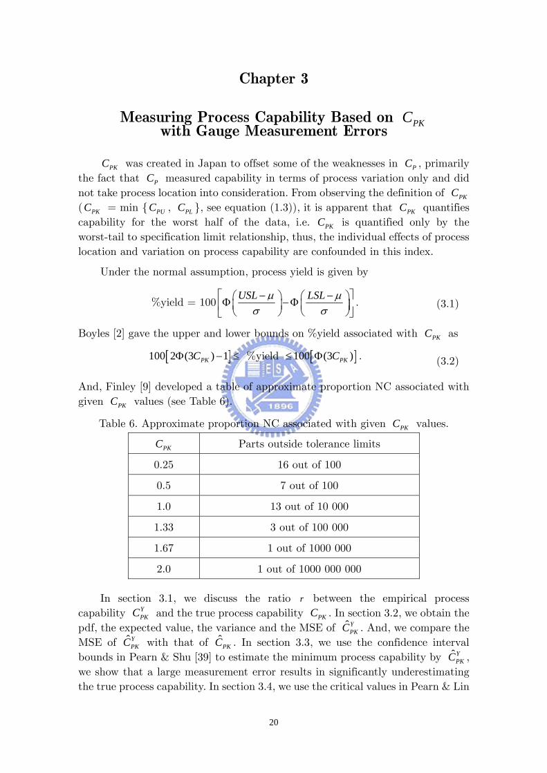
Chapter 3

Measuring Process Capability Based on PKCwith Gauge Measurement Errors

PKC was created in Japan to offset some of the weaknesses in PC , primarily the fact that PC measured capability in terms of process variation only and did not take process location into consideration. From observing the definition of PKC ( PKC = min { PUC , PLC }, see equation (1.3)), it is apparent that PKC quantifies capability for the worst half of the data, i.e. PKC is quantified only by the worst-tail to specification limit relationship, thus, the individual effects of process location and variation on process capability are confounded in this index.

Under the normal assumption, process yield is given by

%yield = 100 USL LSLμ μσ σ

⎡ ⎤− −⎛ ⎞ ⎛Φ −Φ⎜ ⎟ ⎜⎢ ⎥⎝ ⎠ ⎝⎣ ⎦

⎞⎟⎠

. (3.1)

Boyles [2] gave the upper and lower bounds on %yield associated with PKC as

[ ]100 2 (3 ) 1PKCΦ − ≤ %yield [ ]100 (3 )PKC≤ Φ . (3.2)

And, Finley [9] developed a table of approximate proportion NC associated with given PKC values (see Table 6).

Table 6. Approximate proportion NC associated with given PKC values.

PKC Parts outside tolerance limits

0.25 16 out of 100

0.5 7 out of 100

1.0 13 out of 10 000

1.33 3 out of 100 000

1.67 1 out of 1000 000

2.0 1 out of 1000 000 000

In section 3.1, we discuss the ratio between the empirical process capability and the true process capability . In section 3.2, we obtain the pdf, the expected value, the variance and the MSE of

rY

ˆ YPKC PKC

PKC . And, we compare the MSE of with that of . In section 3.3, we use the confidence interval bounds in Pearn & Shu [39] to estimate the minimum process capability by

ˆ Y ˆˆ Y

PKC PKCPKC ,

we show that a large measurement error results in significantly underestimating the true process capability. In section 3.4, we use the critical values in Pearn & Lin

20

[37] to test whether the process capability meets the requirement, and we show that the α -risk and the power both become decrease with measurement error. In section 3.5, we present our modified confidence interval bounds and critical values for the cases that measurement errors are unavoidable. Finally in section 3.6, an example is presented.

3.1 Empirical Process Capability YPKC

Suppose that X ~ Normal ( μ , 2σ ) represents the relevant quality characteristic of a manufacturing process, and PKC measures the true process capability. However in practice, the observed variable is measured rather than the true variable

YX . Assume that X and M are stochastically independent,

we have ~ Normal (Y μ , 2Yσ = 2σ + 2

Mσ ), and the empirical process capability index is obtained after substituting Y

PKC Yσ for σ . The relationship between the true process capability PKC and the empirical process capability can be expressed as

YPKC

2 2

1

1

YPK

PK P

CC Cλ

=+

. (3.3)

Since the variation of data we observed is larger than the variation of the original data, the denominator of the index PKC becomes larger, and the true capability of the process is understated if calculation of process capability index is based on empirical data . Y

Figure 7(a). Surface plot of with r

PC [1, 2] for ∈ λ [0, 0.5]. ∈

Figure 7(b). Plots of versus r λ [0, 0.5] for

∈PC = 1.0(0.2)2.0.

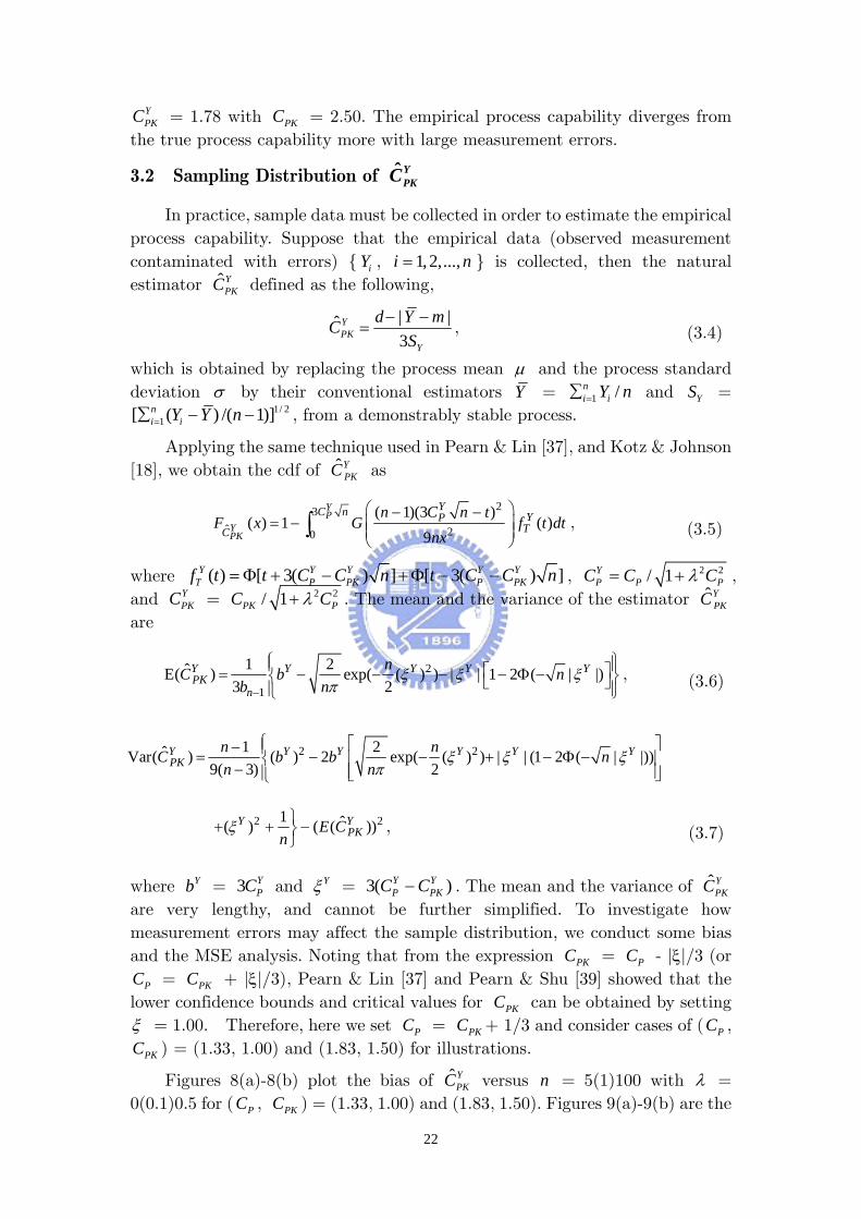
Figure 7(a) displays the surface plot of the ratio = for r /PK PKC CY λ ∈ [0, 0.5] with PC ∈ [1, 2]. Figure 7(b) plots the ratio versus r λ for PC = 1.0(0.2)2.0. Those figures show that the measurement errors result in a decrease in the estimate. Small process variation has the same effect as the presence of measurement error does. Since r would be small if λ becomes large, the gauge becomes more important as the true capability improves. For instance, If λ = 0.5 and PC = 2 (the ratio = 0.71), = 0.36 with = 0.50, and r Y

PKC PKC

21

YPKC = 1.78 with = 2.50. The empirical process capability diverges from

the true process capability more with large measurement errors. PKC

3.2 Sampling Distribution of ˆ YPKC

In practice, sample data must be collected in order to estimate the empirical process capability. Suppose that the empirical data (observed measurement contaminated with errors) { , iY 1,2,...,i n= } is collected, then the natural estimator defined as the following, ˆ Y

PKC

ˆ YPKC | |

3− −

=Y

d Y mS

, (3.4)

which is obtained by replacing the process mean μ and the process standard deviation σ by their conventional estimators Y = and = 1 /=∑n

i iY n YS1/ 2

1[ ( ) /( 1)]ni iY Y n=∑ − − , from a demonstrably stable process.

Applying the same technique used in Pearn & Lin [37], and Kotz & Johnson [18], we obtain the cdf of ˆ Y

PKC as

23ˆ 20

( 1)(3 )( ) 1 ( )

9

YP

YPK

YC n YPTC

n C n tF x G f

nx

⎛ ⎞− −= − ⎜ ⎟⎜ ⎟

⎝ ⎠∫ t dt , (3.5)

where ( ) [ 3( ) ] [ 3( ) ]Y Y Y Y YT P PK P PKf t t C C n t C C n= Φ + − +Φ − − , 2 2/ 1Y

P P PC C Cλ= + , and = Y

PKC 2 2/ 1PKC λ+ PC . The mean and the variance of the estimator ˆ YPKC

are

2

1

1 2ˆE( ) exp( ( ) ) | | 1 2 ( | |)3 2

Y Y Y YPK

n

nC b nb n

ξ ξ ξπ−

⎧ ⎫⎪ ⎪Y⎡ ⎤= − − − − Φ −⎨ ⎬⎣ ⎦⎪ ⎪⎩ ⎭, (3.6)

2 21 2ˆVar( ) ( ) 2 exp( ( ) ) | | (1 2 ( | |))9( 3) 2

Y Y Y Y YPK

n nC b b nn n

ξ ξ ξπ

⎧ ⎡ ⎤− ⎪= − − + − Φ −⎢ ⎥⎨− ⎢ ⎥⎪ ⎣ ⎦⎩

Y

2 21 ˆ( ) ( ( ))Y YPKE C

nξ ⎫+ + −⎬

⎭, (3.7)

where = 3 and Yb YPC Yξ = 3( . The mean and the variance of

are very lengthy, and cannot be further simplified. To investigate how measurement errors may affect the sample distribution, we conduct some bias and the MSE analysis. Noting that from the expression

)Y YP PKC C− ˆ Y

PKC

PKC = PC - |ξ|/3 (or PC = PKC + |ξ|/3), Pearn & Lin [37] and Pearn & Shu [39] showed that the

lower confidence bounds and critical values for PKC can be obtained by setting ξ = 1.00. Therefore, here we set PC = PKC + 1/3 and consider cases of ( PC ,

PKC ) = (1.33, 1.00) and (1.83, 1.50) for illustrations.

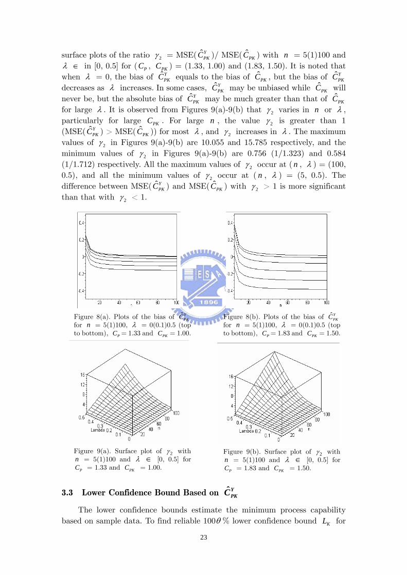
Figures 8(a)-8(b) plot the bias of ˆ YPKC versus = 5(1)100 with n λ =

0(0.1)0.5 for ( PC , PKC ) = (1.33, 1.00) and (1.83, 1.50). Figures 9(a)-9(b) are the

22

surface plots of the ratio 2γ = MSE( ˆ YPKC )/ MSE( ˆ

PKC ) with = 5(1)100 and nλ in [0, 0.5] for (∈ PC , PKC ) = (1.33, 1.00) and (1.83, 1.50). It is noted that when λ = 0, the bias of equals to the bias of , but the bias of decreases as

ˆ YPKC ˆ

PKC ˆ YPKC

λ increases. In some cases, ˆ YPKC may be unbiased while ˆ

PKC will never be, but the absolute bias of ˆ Y

PKC may be much greater than that of ˆPKC

for large λ . It is observed from Figures 9(a)-9(b) that 2γ varies in or n λ , particularly for large PKC . For large , the value n 2γ is greater than 1 (MSE( ˆ Y

PKC ) > MSE( ˆPKC )) for most λ , and 2γ increases in λ . The maximum

values of 2γ in Figures 9(a)-9(b) are 10.055 and 15.785 respectively, and the minimum values of 2γ in Figures 9(a)-9(b) are 0.756 (1/1.323) and 0.584 (1/1.712) respectively. All the maximum values of 2γ occur at ( , n λ ) = (100, 0.5), and all the minimum values of 2γ occur at ( , n λ ) = (5, 0.5). The difference between MSE( ˆ Y

PKC ) and MSE( ˆPKC ) with 2γ > 1 is more significant

than that with 2γ < 1.

Figure 8(a). Plots of the bias of ˆ Y

PKC for = 5(1)100, n λ = 0(0.1)0.5 (top to bottom), PC = 1.33 and PKC = 1.00.

Figure 8(b). Plots of the bias of ˆ Y

PKC for = 5(1)100, n λ = 0(0.1)0.5 (top to bottom), PC = 1.83 and PKC = 1.50.

Figure 9(a). Surface plot of 2γ with

= 5(1)100 and n λ [0, 0.5] for ∈PC = 1.33 and PKC = 1.00.

Figure 9(b). Surface plot of 2γ with

= 5(1)100 and n λ [0, 0.5] for ∈PC = 1.83 and PKC = 1.50.

3.3 Lower Confidence Bound Based on ˆ YPKC

The lower confidence bounds estimate the minimum process capability based on sample data. To find reliable 100θ % lower confidence bound KL for

23

PKC (θ represents the probability that the confidence interval contains the actual PKC ), Pearn & Shu [39] solved the following equation,

2

20

( 1)( )ˆ9 ( )

b n

PK

n b n tGn C

⎛ ⎞− −⎜ ⎟⎜ ⎟⎝ ⎠

∫ ( )⎡Φ +⎣ t nξ ( )⎤+Φ − ⎦t nξ 1dt θ= − . (3.8)

Noting that = b 3 PC can be expressed as = b 3 |KL |ξ+ . Since the process parameters μ and σ are unknown, then the distribution characteristic parameter ξ = ( ) /mμ σ− is also unknown. To eliminate the need for further estimating the distribution characteristic parameter ξ , Pearn & Shu [39] examined the behavior of the lower confidence bound KL against the parameter ξ . They performed extensive calculations to obtain the lower confidence bound values KL for ξ = 0(0.05)3.00, = 0.7(0.1)3.0, = 10(5)200 with confidence coefficient

ˆPKC n

θ = 0.95. They found that the lower confidence bound KL obtains its minimum at ξ = 1.00 in all cases. Thus for practical purpose

they recommended to solve equation (3.8) with ξ = ξ̂ = 1.00 to obtain the required lower confidence bounds, without having to further estimate the parameter ξ .

But, is substituted into equation (3.8) to obtain the confidence bounds, which can be written as (we denote the bound originated from

ˆ YPKC

ˆ YPKC as

YKL ),

2(3 1)

20

( 1)[(3 1) ]ˆ9 ( )

YK

YL n KYPK

n L n tGn C

+ ⎛ ⎞− + −⎜ ⎟⎜ ⎟⎝ ⎠

∫ ( )t n⎡Φ +⎣ ( )t n ⎤+Φ − ⎦ 1dt θ= − . (3.9)

The confidence coefficient by the confidence bound YKL (denoted by Yθ ) is

2(3 )

20

( 1)[(3 ) ]1 ˆ9 ( )

Y YK

Y YL nY KYPK

n L n tGn C

ξ ξθ+ ⎛ ⎞− + −

= − ⎜ ⎟⎜ ⎟⎝ ⎠

∫ ˆ( )Yt nξ⎡Φ +⎣ˆ( )Yt nξ ⎤+Φ − ⎦ dt ,

(3.10)

where Yξ = 3( )P PKC C− , and Yξ = 3( ). Since is smaller than ˆYPC ˆ Y

PKC− ˆ YPKC

ˆPKC , and Y

KL is smaller than KL , then Yθ is always greater than θ . Figures 10(a)-10(b) plot Y

KL versus λ ∈ [0, 0.5] with = 50, n ˆPKC = 1.00, 1.50, and

= + ˆPC ˆ

PKC 3γ , 3γ = 0.33, 0.50, 0.67, and 1.00 for 95% confidence intervals (for sufficiently large sample size , we have n ˆ Y

PKC = ˆPKC / 2 2ˆ1 PCλ+ .

Therefore, we set ˆ YPKC = ˆ

PKC / 2 2ˆ1 PCλ+ to obtain ˆ YPKC in Figures

10(a)-10(b)). We see that in Figures 10(a)-10(b), YKL decreases in λ , especially

for large ˆPC values, and the decrement of Y

KL is more significant for large ˆPKC .

A large measurement error results in significantly underestimating the true process capability.

In current practice, a process is called “inadequate” if PKC < 1.00, “marginally capable” if 1.00 < PKC < 1.33, “satisfactory” if 1.33 < PKC < 1.50, “excellent” if 1.50 < PKC < 2.00, and “super” if 2.00 < PKC . If capability

24

measures do not include the measurement errors, significant underestimation of the true process capability may result in high production cost, losing the power of competition. For instance, suppose that a process has a 95% lower confidence bound, 1.236 ( ˆ

PKC = 1.50) with = 50, which meets the threshold of an “excellent” process. But the bound may be calculated as 0.983 with measurement errors

n

λ = 0.30 and the process is determined as “inadequate”.

Figure 10(a). Plots of Y

KL versus λ with = 50 for n ˆPC = 1.33, 1.50, 1.67, 2.00 (top to bottom) and ˆPKC = 1.00.

Figure 10(b). Plots of Y

KL versus λ with = 50 for n ˆPC = 1.83, 2.00, 2.17, 2.50 (top to bottom) and ˆPKC = 1.50.

3.4 Capability Testing Based on ˆ YPKC

To determine if a given process meets the preset capability requirement, we could consider the statistical testing with null hypothesis : (process is not capable) and alternative hypothesis : > c (process is capable), where is the required process capability. If the calculated process capability is greater than the corresponding critical value, we reject the null hypothesis and conclude that the process is capable. Suppose that the nominal size of the statistical testing is

0H PKC ≤ c0H PKC

c

α , the critical value can be determined by solving the following equation,

0c

23

20

( 1)(3 )[ 3( ) ] [ 3( ) ]

9PC n P

P Po

n C n tG t C c n t C c

ncn dt α

⎛ ⎞− − ⎡ ⎤Φ + − + Φ − − =⎜ ⎟ ⎣ ⎦⎜ ⎟⎝ ⎠

∫

(3.11)

with test power

( )0ˆ( ) | ,PK PK PK PC P C c C Cπ = ≥

23

20

( 1)(3 )[ 3( ) ] [ 3( ) ]

9PC n P

P PK P PKo

n C n tG t C C n t C

nc

⎛ ⎞− −C n dt⎡ ⎤= Φ + − + Φ −⎜ ⎟ −⎣ ⎦⎜ ⎟

⎝ ⎠∫ .

(3.12)

25

To eliminate the need for estimating the characteristic parameter PC , Pearn & Lin [37] examined the behavior of the critical values against the parameter

0cPC . They performed extensive calculations to obtain the critical

values for 0c PC = (0.01)( c +1), = 1.00, 1.33, 1.50, 1.67, and 2.00, = 10 (50) 300, and

c c nα = 0.05. They found that the critical values obtains its

maximum at 0c

PC = + 1/3 in all cases. For practice purpose, they recommended to solve equation (3.11) with

cPC = + 1/3 to obtain the

required critical values, without having to further estimate the parameter c

PC .

Thus, the α -risk corresponding to the test using the sample estimate ˆ Y

PKC (denoted by Yα ) will become

( )0ˆ | , 1= ≥ = = +Y Y

PK PK PP C c C c C cα / 3

23

20

( 1)(3 )[ 3( ) ] [ 3( ) ]

9

YP

YC n Y Y Y YPP PK P PK

o

n C n tG t C C n t C

nc

⎛ ⎞− −C n dt⎡ ⎤= Φ + − + Φ −⎜ ⎟ −⎣ ⎦⎜ ⎟

⎝ ⎠∫ ,

(3.13)

where = YPC 2( 1/3) / 1 ( 1/3)+ + +c cλ 2 , and = Y

PKC 2/ 1 ( 1/ 3)+ +c cλ 2 . The test power (denoted by Yπ ) is

( )0ˆ | , 1/ 3Y Y

PK PK PP C c C C cπ = ≥ = +

23

20

( 1)(3 )[ 3( ) ] [ 3( ) ]

9

YP

YC n Y Y Y YPP PK P PK

o

n C n tG t C C n t C

nc

⎛ ⎞− −C n dt⎡ ⎤= Φ + − + Φ −⎜ ⎟ −⎣ ⎦⎜ ⎟

⎝ ⎠∫ ,

(3.14)

where = YPC 2 2( 1/3)/ 1 ( 1/3+ + +PK PKC Cλ ) , and = Y

PKC 2 2/ 1 ( 1/3)+ +PK PKC Cλ .

Earlier discussions indicate that the true process capability would be severely underestimated if ˆ Y

PKC is used. The probability that ˆ YPKC is greater

than would be less than that of using 0c ˆPKC . Thus, the α -risk using ˆ Y

PKC is less than the α -risk if using when estimating ˆ

PKC PKC . The test power if using ˆ

PKC is also less than the test power of using ˆPKC . That is, Yα ≤ α and

Yπ ≤ π . Figures 11(a)-11(b) are the surface plots of Yα with = 5(1)100, nλ ∈ [0, 0.5] for = 1.00, 1.50, and c α = 0.05. Figures 12(a)-12(b) plot Yπ versus λ with = 50, n α = 0.05, for = 1.00, 1.50, and c PKC =

(0.20)( +1). Note that for c c λ = 0, Yα = α and Yπ = π . In Figures 11(a)-11(b), Yα decreases as λ or increases, and the decreasing rate is more significant with large . In fact, for large

nc λ , Yα is smaller than 51 10−× .

In Figures 12(a)-12(b), Yπ decreases as λ increases, but increases as n increases. Decrement of Yπ in λ is more significant for large . In the presence of measurement errors,

cYπ may decrease substantially. For instance,

in Figure 12(b), the Yπ value ( = 1.50, = 50) for c n PKC = 2.30 is Yπ =

26

0.994 if there is no measurement error (λ = 0). But, when λ = 0.5, Yπ decreases to 0.012, the decrement of the power is 0.982.

Figure 11(a). Surface plot of Yα with

= 5(1)100 and n λ [0, 0.5] for = 1.00 and

∈ cα = 0.05.

Figure 11(b). Surface plot of Yα with

= 5(1)100 and n λ [0, 0.5] for = 1.50 and

∈ cα = 0.05.

Figure 12(a). Plots of Yπ versus λ with = 50, n α = 0.05 for = 1.00, c

PKC = 1.00(0.20)2.00 (bottom to top).

Figure 12(b). Plots of Yπ versus λ with = 50, n α = 0.05 for = 1.50, c

PKC = 1.50(0.20)2.50 (bottom to top).

3.5 Modified Confidence Bounds and Critical Values

We showed earlier that the coefficients increase due to underestimating the lower confidence bounds. We also showed that the α -risk and the test power decrease with measurement error. The probability of passing non-conforming product units decreases, but the probability of correctly judging a capable process as incapable also decreases. Since the lower confidence bound is severely underestimated and the power becomes small, the producers cannot firmly state that their processes meet the capability requirement even if their processes are sufficiently capable. Good product units would be incorrectly rejected in this case. Unnecessary cost may accompany those incorrect decisions to the producers. Improving the gauge capability and training the operators by proper education are essential to measurement error reduction. Nevertheless, measurement errors are unavoidable in most industry applications. In this section, we consider the adjustment of confidence bounds and critical values to

27

provide better capability assessment.

Suppose that the desired confidence coefficient is θ , the adjusted confidence interval of PKC with lower confidence bound KL∗ , can be established as

( )PK KP C Lθ ∗= >

2

20

( 1)( )1 ˆ9 ( )

b n

YPK

n b n tGn C

∗ ∗⎛ ⎞− −= − ⎜ ⎟⎜ ⎟

⎝ ⎠∫ ˆ( )⎡Φ +⎣

Yt nξ ˆ( )⎤+Φ − ⎦Yt nξ dt , (3.15)

where = b∗ 2 23 / 1 | YK PL C |λ ξ∗ + + . To eliminate the need for estimating the

characteristic parameter Yξ , we follow the method of Pearn and Shu [39] by setting Yξ = 1.00 to find the adjusted lower confidence bound KL∗ , where PC can be obtained by equation 2 23( ) / 1P KC L Cλ∗− + P = 1.00, as

2 2 2

12

18 324 4(9 )(9 1)2(9 )

K K KP P

L L LC C

λλ

∗ ∗ ∗+ − − −= =

− (3.16)

Figures 13(a)-13(b) are comparisons among KL , YKL , and KL∗ for ˆ

PKC = 1.00, 1.50 with = 50, where n KL is the 95% lower confidence bound using

, ˆPKC Y

KL is the 95% lower confidence bound using , and ˆ YPKC KL∗ is the

adjusted 95% lower confidence bound using ˆ YPKC ( ˆ Y

PKC = ˆPKC / 2 2ˆ1 PCλ+ is

also used to obtain ˆ YPKC ). In this case, the probability that the lower confidence

interval with bound YKL contains the actual PKC value is greater than that of

the interval with the bound KL or KL∗ , while the probability that the lower confidence interval with bound KL or KL∗ contains the actual PKC value is 0.95. From Figures 13(a)-13(b), we see that the lower confidence bounds remained underestimated, even if it is adjusted. But, the magnitude of underestimation using the adjusted confidence bound is significantly reduced.

Figure 13(a). Plots of KL , KL∗ , and

YKL (top to bottom) versus λ with = 50 and for n ˆ

PKC = 1.00.

Figure 13(b). Plots of KL , KL∗ , and

YKL (top to bottom) versus λ with = 50 and for n ˆ

PKC = 1.50.

28

In order to improve the test power, we revise the critical values to satisfy < . Thus, the probability {

0c∗

0c∗ 0c P ˆ YPKC > 0c∗ } is greater than

{ > }. Both the P ˆ YPKC 0c α -risk and the test power increase when we use as a

new critical value in the testing. Suppose that the 0c∗

α -risk using the revised critical value is 0c∗ α ∗ , the revised critical values 0c∗ can be determined by

( )0ˆ |Y

PK PKP C c C cα∗ ∗= ≥ =

23

20

( 1)(3 )[ 3( ) ] [ 3( ) ]

9 ( )

YP

YC n Y Y Y YPP PK P PK

o

n C n tG t C C n t C

n c∗⎛ ⎞− −

= Φ + − + Φ −⎜ ⎟⎜ ⎟⎝ ⎠

∫ C n dt− ,

(3.17)

where 2 2/ 1YP P PC C Cλ= + , and = Y

PKC 2 2/ 1 Pc λ+ C . To eliminate the need for further estimating the characteristic parameter PC , we follow the method described in Pearn and Lin [37] by setting = + 1/3 to find the adjusted critical values , where

YPC Y

PKC0c∗ PC can be obtained by the equation 2 2/ 1P PC Cλ+ =

2 2/ 1 Pc λ+ C + 1/3, as

2 2 2

22

18 324 4(9 )(9 1)2(9 )P P

c c cC C

λλ

+ − − −= =

−. (3.18)

To ensure that the α -risk is within the preset magnitude, we let α∗ = α and solve the equation to obtain 0c∗ . The power (denoted by π ∗ ) can be calculated as

( )0 2ˆ( ) | ,Y

PK PK PK P PC P C c C C Cπ ∗ = ≥ =

23

20

( 1)(3 )( ) ( )

9 ( )

YP

YC n P

o

n C n tG t n

n c∗⎛ ⎞− −

t n dt⎡ ⎤= Φ +⎜ ⎟ + Φ −⎣ ⎦⎜ ⎟⎝ ⎠

∫ , (3.19)

where = + 1/3, and = YPC Y

PKC YPKC 2 2

2/ 1PK PC Cλ+ .

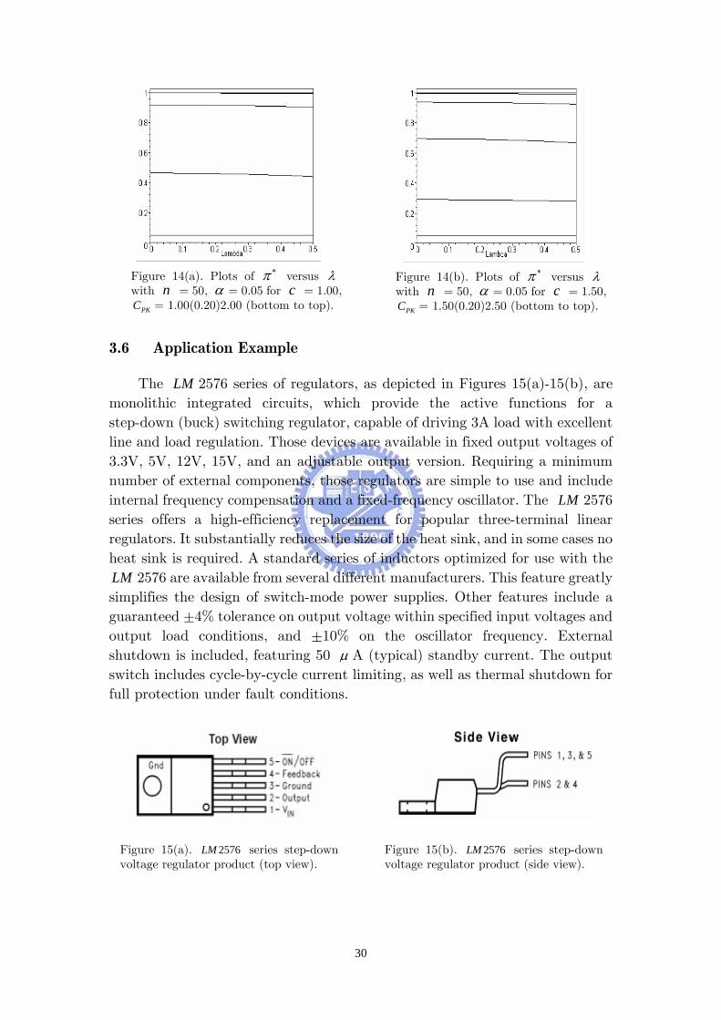
Figures 14(a)-14(b) are plots of π ∗ versus λ with = 50, n α = 0.05, for = 1.00, 1.50 and c PKC = (0.20)(c +1). From those figures, we see that the powers corresponding to the adjusted critical values

c0c∗ remain decreasing

in measurement error, but the decrements are much smaller. We improve the test power to a certain degree. For instance, when we compare the Yπ values in Figure 12(b) ( = 1.50, = 50) to the c n π ∗ values in Figure 14(b) ( = 1.50,

= 50), we obtain that c

n Yπ = 0.012 and π ∗ = 0.992 with λ = 0.5. In this case, using the adjusted critical values 0c∗ , we improve the test power by 0.980 (which is rather significant). For our results to be practical, we tabulate the revised critical values for some commonly used capability requirements in Tables 16-19 in the Appendix. Using those tables, the practitioner may omit the complex calculation and simply select the proper critical values for capability testing.

29

Figure 14(a). Plots of π ∗ versus λ with = 50, n α = 0.05 for = 1.00, c

PKC = 1.00(0.20)2.00 (bottom to top).

Figure 14(b). Plots of π ∗ versus λ with = 50, n α = 0.05 for = 1.50, c

PKC = 1.50(0.20)2.50 (bottom to top).

3.6 Application Example

The LM 2576 series of regulators, as depicted in Figures 15(a)-15(b), are monolithic integrated circuits, which provide the active functions for a step-down (buck) switching regulator, capable of driving 3A load with excellent line and load regulation. Those devices are available in fixed output voltages of 3.3V, 5V, 12V, 15V, and an adjustable output version. Requiring a minimum number of external components, those regulators are simple to use and include internal frequency compensation and a fixed-frequency oscillator. The LM 2576 series offers a high-efficiency replacement for popular three-terminal linear regulators. It substantially reduces the size of the heat sink, and in some cases no heat sink is required. A standard series of inductors optimized for use with the LM 2576 are available from several different manufacturers. This feature greatly simplifies the design of switch-mode power supplies. Other features include a guaranteed ±4% tolerance on output voltage within specified input voltages and output load conditions, and ±10% on the oscillator frequency. External shutdown is included, featuring 50 μ A (typical) standby current. The output switch includes cycle-by-cycle current limiting, as well as thermal shutdown for full protection under fault conditions.

Figure 15(a). series step-down voltage regulator product (top view).

2576LM

Figure 15(b). series step-down voltage regulator product (side view).

2576LM

30

Table 7. 70 observations for output voltage (unit: V)

3.292 3.289 3.293 3.323 3.279 3.304 3.306 3.288 3.287 3.319

3.299 3.269 3.300 3.294 3.308 3.285 3.292 3.278 3.285 3.282

3.297 3.278 3.311 3.295 3.319 3.303 3.305 3.326 3.315 3.298

3.321 3.315 3.284 3.319 3.302 3.314 3.308 3.303 3.294 3.312

3.297 3.305 3.306 3.295 3.286 3.293 3.288 3.314 3.318 3.295

3.309 3.296 3.296 3.305 3.293 3.298 3.305 3.289 3.288 3.315

3.308 3.279 3.292 3.293 3.265 3.283 3.307 3.314 3.303 3.305

Consider a supplier manufacturing step-down voltage regulator products in

Taiwan, making LM 2576-3.3 type with specifications of output voltage: = 3.3V, = 3.366V, = 3.234V for conditions of = 12V (input voltage), = 0.5A (load current), and

TUSL LSL INV

LOADI JT = 25 (temperature). A total of 70 observations are collected and displayed in Table 7. Histogram and normal probability plot show that the collected data follows the normal distribution. Shapiro-Wilk test is applied to further justify the assumption. To determine whether the process is “excellent” ( > 1.50) with unavoidable measurement errors

0 C

PKCλ = 0.25, we first determine that = 1.50 and c α = 0.05. Then, based

on the sample data of 70 observations, we obtain the sample mean Y = 3.299, the sample standard deviation = 0.013, and the point estimator YS ˆ Y

PKC = 1.632. From Table A7, we obtain the critical value 0c∗ = 1.595 based on α , λ and . Since n ˆ Y

PKC > , we therefore conclude that the process is “excellent”. Moreover, by inputting

0c∗ˆ Y

PKC , λ , , and the desired confidence coefficient n θ = 0.95 into the computer program we obtain the 95% lower confidence bound of the true process capability as 1.542. We can see that if we ignore the measurement errors and evaluate the critical value without any correction, the critical value may be calculated as = 1.758. In this case would reject that the process is “excellent” since

0cˆ Y

PKC is no greater than the uncorrected critical value 1.758.

31