81
Chapter 3 Optimization Paisan Nakmahachalasint

Chapter 3Optimization
Paisan Nakmahachalasint

Optimization Problems
The basic optimization model is
Optimize fj(X) for j in J
subject to
gi(X) bi for all i in I.
We seek the vector X0 giving the optimal value for the set of function fj(X).
⎧ ⎫⎪ ⎪≥⎪ ⎪⎪ ⎪⎪ ⎪=⎨ ⎬⎪ ⎪⎪ ⎪≤⎪ ⎪⎪ ⎪⎩ ⎭
Optimization Problems
The vector X are called the decision variables of the model.The function fj(X) are called the objective functions.The conditions that the decision variables must satisfy are called constraints.

Optimization Problems
There are various ways of classifying optimization problems. These classification are not meant to be mutually exclusive but to describe mathematical characteristics possessed by the problem.An optimization is said to be unconstrained if there are no constraints and constrained if one or more conditions are present.

Linear Programming
An optimization problem is said to be a linear program if it satisfied the following properties:
There is a unique objective function.
Whenever a decision variable appears in either the objective function or one of the constraint functions, it must appear only as a power term with an exponent of 1, possibly multiplied by a constant.

Linear Programming
No term in the objective function or in any of the constraints can contain products of the decision variables.
The coefficients of the decision variables in the objective function and each constraint are constant.
The decision variables are permitted to assume fractional as well as integer values.

Variants of Problems
Problems that are probabilistic in nature are called stochastic programs.If all decision variable are restricted to integer values, the problem is called an integer program. If the integer restriction applies to only a subset of the decision variables, then it is called a mixed-integer program.

Example
Determining a Production Schedule
A carpenter makes tables and bookcases. He wishes to determine a weekly production schedule that maximizes his profits. It costs $5 and $7 to produce tables and bookcases, respectively.

Example
Consider a variation where the carpenter realizes the following information
Each week he has up to 690 board-feet of lumber and up to 120 hours of labor.
430$30Bookcase
520$25Table
Labor(hours)
Lumber(board-feet)
Unit Profit
Example
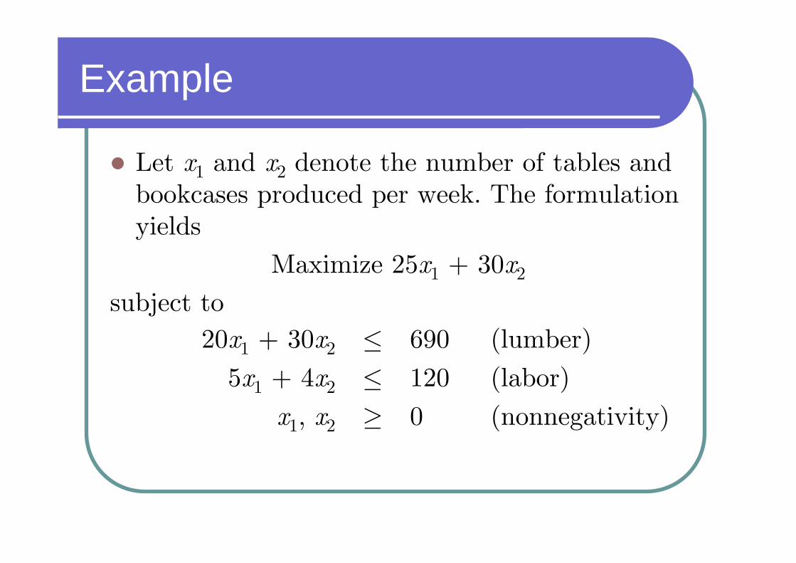
Let x1 and x2 denote the number of tables and bookcases produced per week. The formulation yields
Maximize 25x1 + 30x2
subject to
(nonnegativity)0≥x1, x2
(labor)120≤5x1 + 4x2
(lumber)690≤20x1 + 30x2
A Graphical Method
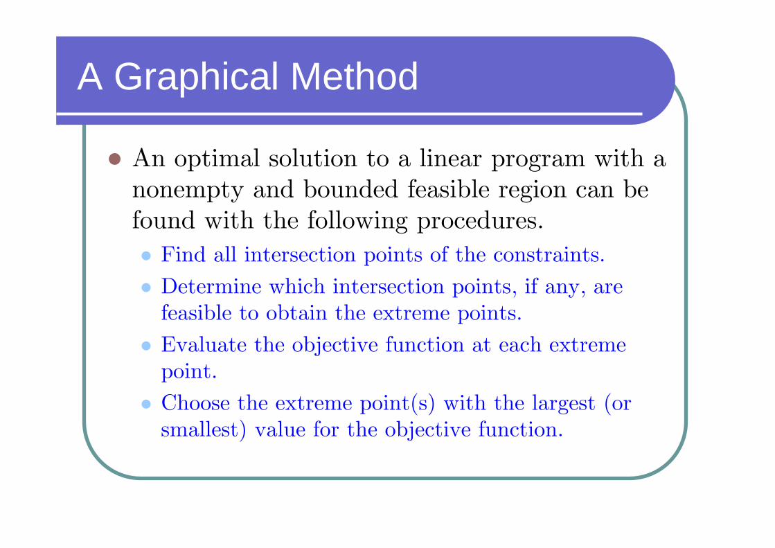
An optimal solution to a linear program with a nonempty and bounded feasible region can be found with the following procedures.
Find all intersection points of the constraints.Determine which intersection points, if any, are feasible to obtain the extreme points.
Evaluate the objective function at each extreme point.Choose the extreme point(s) with the largest (or smallest) value for the objective function.

A Graphical Method
(0, 30)
1x
2x
(0, 0)A (24, 0)B (34.5, 0)
(12,15)C
(0,23)D
1x1y
2x 2y
0≥x1, x2, y1, y2
120=5x1 + 4x2 + y2
690=20x1 + 30x2 + y1
-52.50034.5(34.5,0)
0-210300(0,30)
280230D (0,23)
001512C (12,15)
0250024B (24,0)
12069000A (0,0)
y2y1x2x1
x1, x2 = decision variablesy1, y2 = slack variables

Complexity
Intersection Point EnumerationSuppose we have a linear program with m
nonnegative decision variables and nconstraints of the form ≤. We add n slack variables, yi, to the constraints to get a total of m + n nonnegative variables. Each intersection point can be determined by choosing m of the variables and set them to 0.
There are possible choices to consider.( )!! !
m nm n
+

The Simplex Method
So far we find an optimal point by searching among feasible intersection points.
The search can be improved by starting with an initial feasible point and moving to a “better” solution until an optimal one is found.
The simplex method incorporates both optimality and feasibility tests to find the optimal solution(s) if one exists.

The Simplex Method
An optimality test shows whether an intersection point corresponds to a value of the objective function better than the best value found so far.A feasibility test determines whether the proposed intersection point is feasible.
The decision and slack variables are separated into two nonoverlapping sets, which we call the independent and dependent sets.

The Simplex Method
Write the carpenter’s problem as
Begin with an initial extreme point x1=x2=0.We determine that y1 = 690, y2 = 120, z = 0.Then x1 and x2 are independent variableswhere y1, y2, and z are dependent variables.
0=–25x1 – 30x2 + z
120=5x1 + 4x2 + y2
690=20x1 + 30x2 + y1

The Simplex Method
If either x1 and x2 is increased, z will increase.
We choose to increase x2 to the maximum possible value as not to violate the constraints.At this stage, x2 is called the entering variable.
The first equation implies that
The second equation implies that
We increase x2 to 23, then y1 = 0.At this stage, y1 is called the exiting variable.
2
69023.
30x ≤ =
2
12030.
4x ≤ =

The Simplex Method
x1 and y1 become the independent variables,x2 and y2 become the dependent variables.
All equations must be adjusted to reflect the changes in the independent and dependent variables.
2 13 301 2 1
7 23 151 1 2
1 1
23
28
5 690
x x y
x y y
x y z
+ + =
− − + =
− + + =

The Simplex Method
We merely need to know the coefficients of the variables with the right-hand side. It is more convenient to record the numbers in a table format, or a tableau.
0
120
690
RHS
1
0
0
z
00–30–25
120/4 = 301045
690/30 = 23013020
y2y1x2x1

The Simplex Method
690
28
23
RHS
1
0
0
z
010–5
28/(7/3) = 121– 2/1507/3
23/(2/3) = 34.501/3012/3
y2y1x2x1
750
12
15
RHS
1
0
0
z
z15/75/700
x13/7– 2/3501
x2– 2/71/1410
y2y1x2x1

Numerical Search Methods
It may be impossible algebraically to solve for a maximum or a minimum using calculus.
Various search methods permit us to approximate solutions to nonlinear optimization problems with a single independent variable.A unimodal function on an interval has exactly one point where a maximum or minimum occurs in the interval.
Numerical Search Methods
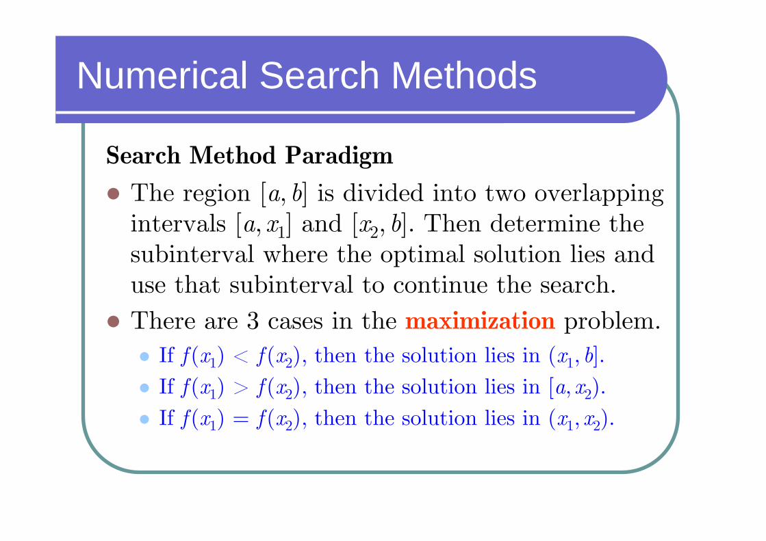
Search Method ParadigmThe region [a, b] is divided into two overlapping intervals [a, x1] and [x2, b]. Then determine the subinterval where the optimal solution lies and use that subinterval to continue the search.There are 3 cases in the maximization problem.
If f (x1) < f (x2), then the solution lies in (x1, b].If f (x1) > f (x2), then the solution lies in [a, x2).If f (x1) = f (x2), then the solution lies in (x1, x2).

Dichotomous Search Method
The Dichotomous Search Method computes
the midpoint , and then moves slightly to
either side of the midpoint to compute two test
points: , where ε is a very small
number. The objective being to place the two test points as close together as possible. The procedure continues until it gets within some small interval containing the optimal solution.
2a b+
2a b
ε+
±

Dichotomous Search Method
Dichotomous Search Algorithm to maximize f(x) over the interval [a,b]
STEP 1: Initialize: Choose a small number ε > 0, such as 0.01. Select a small t such that 0 < t < b – a, called the length of uncertaintyfor the search. Calculate the number of iterations n using the formula
ln(( )/ ).
ln 2b a t
n⎡ ⎤−⎢ ⎥=⎢ ⎥⎢ ⎥

Dichotomous Search Method
STEP 2: For k = 1 to n, do Steps 3 and 4.
STEP 3:
STEP 4: (For a mximization problem)If f (x1) ≥ f (x2) , then b = x2 else a = x1.k = k + 1Return to Step 3.
STEP 5: Let
1 2and2 2
a b a bx xε ε
⎛ ⎞ ⎛ ⎞+ +⎟ ⎟⎜ ⎜= − = +⎟ ⎟⎜ ⎜⎟ ⎟⎜ ⎜⎝ ⎠ ⎝ ⎠
* *and ( )2
a bx MAX f x
+= =

Dichotomous Search Method
In stead of determining the number of iterations, we may wish to continue until the change in the dependent variable is less than some predetermined amount, say Δ. That is continue to iterate until f (a) – f (b) ≤ Δ.To minimize a function y = f (x), either maximize –y or switch the directions of the signs in Step 4.

Dichotomous Search Method
ExampleMaximize f(x) = –x2 – 2x over the interval
–3 ≤ x ≤ 6. Assume the optimal tolerance to be less than 0.2 and we choose ε = 0.01.
We determine the number of iterations to be
⎡ ⎤
6 ( 3)ln
ln 450.2 5.49 6ln 2 ln 2
n
⎡ ⎤⎛ ⎞− − ⎟⎜⎢ ⎥⎟⎜ ⎟⎜⎢ ⎥ ⎡ ⎤⎝ ⎠= ⎢ ⎥ = = =⎢ ⎥
⎢ ⎥ ⎢ ⎥⎢ ⎥ ⎢ ⎥

Dichotomous Search Method
Results of a Dichotomous Search.
– 0.87531– 1.035636
0.9844530.989041– 0.87531– 0.89531– 0.735– 1 .035635
0.9997560.998731– 1.01563– 1.03563– 0.735– 1.316254
0.9122360.899986– 1.29625– 1.31625– 0.735– 1.87753
0.2646940.229994– 1.8575– 1.8775– 0.735– 32
0.9297750.939975– 0.735– 0.7551.51– 31
– 5.3001– 5.20011.511.496– 30
f (x2)f (x1)x2x1ban
* *1.03563 0.875310.95547 and ( ) 0.99802
2x f x
− −= = − =

Golden Section Search Method
The Golden Section Search Method chooses x1and x2 such that the one of the two evaluations of the function in each step can be reused in the next step.
The golden ratio is the ratio r satisfying
r ( )1 r−
1 5 10.618034
1 2r r
rr− −
= ⇒ = ≈

Golden Section Search Method
a b1x 2xx
y2 1
1 21 2
1 1and
r rr r
r r− −
= =
21
x ar
b a−
=−
12
b xr
b a−
=−
1 2
5 12
r r−
= =

Golden Section Search Method
Golden Section Search Method to maximize f (x) over the interval a ≤ x ≤ b.
STEP 1: Initialize: Choose a tolerance t > 0.
STEP 2: Set and define the test points:
STEP 3: Calculate f (x1) and f (x2).
5 12
r−
=
( )( )
( )1
2
1x a r b a
x a r b a
= + − −
= + −

Golden Section Search Method
STEP 4: (For a maximization problem)
If f (x1) ≤ f (x2) then a = x1, x1 = x2
else b = x2, x2 = x1. Find the new x1 or x2using the formula in Step 2.
STEP 5: If the length of the new interval from Step 4 is less than the tolerance t specified, then stop. Otherwise go back to Step 3.
STEP 6: Estimate x* as the midpoint of the final
interval and compute MAX = f (x*)*2
a bx
+=
Golden Section Search Method
To minimize a function y = f (x), either maximize –y or switch the directions of the signs in Step 4.
The advantage of the Golden Section Search Method is that only one new test point must be computed at each successive iteration.
The length of the uncertainty is 61.8% of he length of the previous interval of uncertainty.

Golden Section Search Method
-0.97651-1.0217411
0.9994480.999961-0.97651-0.99379-0.94856-1.0217410
0.9999610.999527-0.99379-1.02174-0.94856-1.066969
0.9973540.999961-0.94856-0.99379-0.87539-1.066968
0.9999610.995516-0.99379-1.06696-0.87539-1.185367
0.9844720.999961-0.87539-0.99379-0.68381-1.185366
0.9000250.984472-0.68381-0.87539-0.37384-1.185365
0.9844720.96564-0.87539-1.18536-0.37384-1.686924
0.6079180.984472-0.37384-0.875390.437694-1.686923
0.9844720.528144-0.87539-1.686920.437694-32
-1.066960.9844720.437694-0.875392.562306-31
-11.69-1.066962.5623060.4376946-30
f (x2)f (x1)x2x1ban
* 0.99913 and 0.999999x MAX= − =

Golden Section Search Method
How small should the tolerance be?If x* is the optimal point, then
If we want the second term to be of a fraction ε of the first term, then
As a rule of thumb, we need
2* * *1( ) ( ) ( )( ) .
2f x f x f x x x′′≈ + −
*
* *2* *
2 ( ).
( ) ( )
f xx x x
x f xε− =
′′
* * .x x xε− ≈
Fibonacci Search Method
If a number of test points is specified in advanced, then we can do slightly better than the Golden Section Search Method.
This method has the largest interval reduction compared to other methods using the same number of test points.
Fibonacci Search Method
nx 1nx − 2nx −
nIαnI
nI1nI −
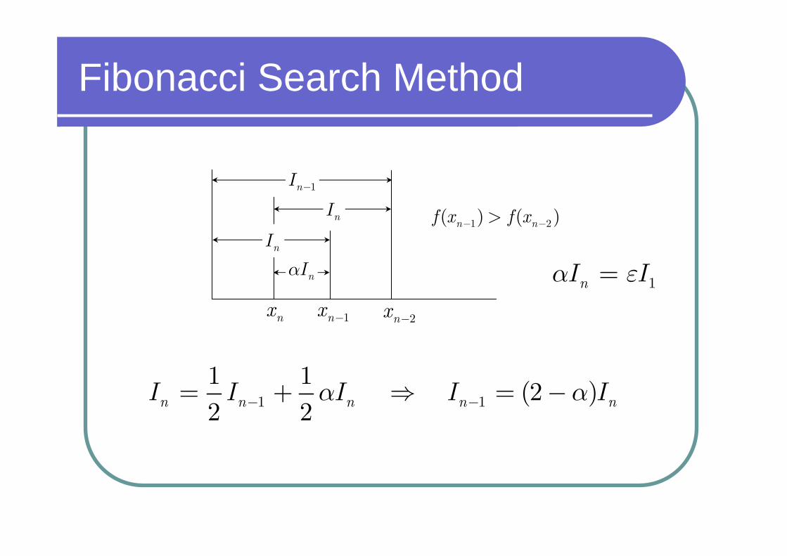
1 2( ) ( )n nf x f x− −>
1 1
1 1(2 )
2 2n n n n nI I I I Iα α− −= + ⇒ = −
1nI Iα ε=
Fibonacci Search Method
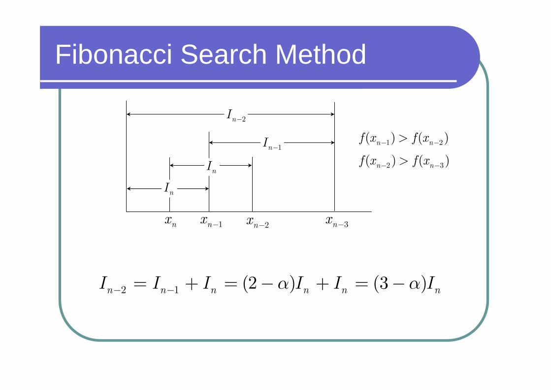
2 1 (2 ) (3 )n n n n n nI I I I I Iα α− −= + = − + = −
nx 1nx − 2nx −
nInI
1 2
2 3
( ) ( )
( ) ( )
n n
n n
f x f x
f x f x
− −
− −
>
>1nI −
3nx −
2nI −

Fibonacci Search Method
1
2 1
3 2 1
4 3 2
2
(2 )
(2 ) (3 )
(3 ) (2 ) (5 2 )
(5 2 ) (3 ) (8 3 )
( )
n n
n n n n n n
n n n n n n
n n n n n n
n k k k n
I I
I I I I I I
I I I I I I
I I I I I I
I F F I
α
α α
α α α
α α α
α
−
− −
− − −
− − −
− +
= −
= + = − + = −
= + = − + − = −
= + = − + − = −
= −
2 1 1 2where , 1k k kF F F F F+ += + = =

Fibonacci Search Method
1x 2x b
2I
1I
a
3I
3I 2I
( ) ( )
( ) ( )1 3 1 3 1 3 1
2 2 2 2 1
n n n n n n
n n n n n n
x a I a F F I a F I F I
x a I a F F I a F I F I
α ε
α ε
− − − −
− −
= + = + + = + +
= + = + + = + +
1 1 1 1 1 1( ) ( )n n n n n nI F F I F I F Iα ε+ − + −= − = −
11
1
1 nn
n
FI I
Fε−
+
⎛ ⎞+ ⎟⎜ ⎟= ⎜ ⎟⎜ ⎟⎜⎝ ⎠

Fibonacci Search Method
If ε = 0, then the formula simplify to
1
1n
n
II
F +
=
( )
( )
11
1
21
n
n
n
n
Fx a b a
F
Fx a b a
F
−
+
+
= + −
= + −
Fibonacci Search Method
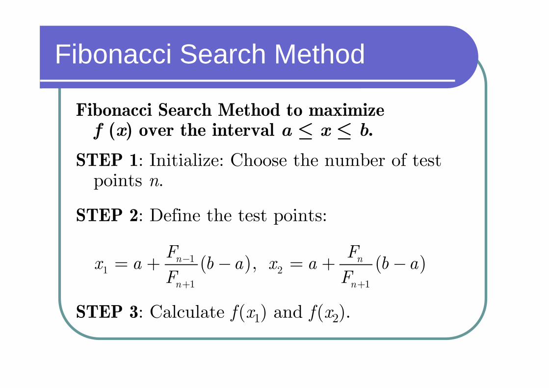
Fibonacci Search Method to maximize f (x) over the interval a ≤ x ≤ b.
STEP 1: Initialize: Choose the number of test points n.
STEP 2: Define the test points:
STEP 3: Calculate f (x1) and f (x2).
( ) ( )11 2
1 1
,n n
n n
F Fx a b a x a b a
F F−
+ +
= + − = + −

Fibonacci Search Method
STEP 4: (For a maximization problem)
If f (x1) ≤ f (x2) then a = x1, x1 = x2
else b = x2, x2 = x1.
n = n – 1. Find the new x1 or x2 using the formula in Step 2.
STEP 5: If n > 1, return to Step 3.
STEP 6: Estimate x* as the midpoint of the final
interval and compute MAX = f (x*)*2
a bx
+=

Fibonacci Search Method
-0.99142-1.0300411
0.9999260.999926-0.99142-0.99142-0.95279-1.0300412
0.9999260.999097-0.99142-1.03004-0.95279-1.0686723
0.9977710.999926-0.95279-0.99142-0.87554-1.0686734
0.9999260.995284-0.99142-1.06867-0.87554-1.1845555
0.9845090.999926-0.87554-0.99142-0.6824-1.1845586
0.8991320.984509-0.6824-0.87554-0.37339-1.18455137
0.9845090.965942-0.87554-1.18455-0.37339-1.6867218
0.6073610.984509-0.37339-0.875540.437768-1.6867349
0.9845090.52845-0.87554-1.68670.437768-35510
-1.067180.9845090.437768-0.875542.562232-38911
-11.6895-1.067182.5622320.4377686-314412
23313
f (x2)f (x
1)x
2x
1baF
nn
* 1.01073 and 0.999885x MAX= − =

Conjugate Gradient Method
We want to find the minimum of the function f(x) of an n-dimensional point x, where we are able to calculate the gradient ∇f(x).
Suppose the function f can be approximated as a quadratic form:
T T1( )
2f c≈ − +x b x x Ax

Conjugate Gradient Method
The number of unknown parameters in the approximation of f is equal to the number of free parameters in A and bwhich is n(n+1)/2 in total.We expect to collect an information content of order n2 numbers before we are able to find the minimum.

Conjugate Gradient Method
We will impose two conditions on the matrix A:
A is symmetric, i.e. A = AT.
A is positive definite, i.e.
which is equivalent to all eigenvalues of Abeging positive.
T 0 for all > ≠x Ax x 0

Conjugate Gradient Method
Note that if A is not symmetric, we may consider (AT+A)/2 instead, that is
Example
( )T T 12
T= +x Ax x A A x
2 24 1 4 2
4 4 63 6 2 6
x xx y x xy y x yy y
⎡ ⎤ ⎡ ⎤⎡ ⎤ ⎡ ⎤⎡ ⎤ ⎡ ⎤⎢ ⎥ ⎢ ⎥⎢ ⎥ ⎢ ⎥= + + =⎢ ⎥ ⎢ ⎥⎢ ⎥ ⎢ ⎥⎢ ⎥ ⎢ ⎥⎣ ⎦ ⎣ ⎦⎣ ⎦ ⎣ ⎦⎢ ⎥ ⎢ ⎥⎣ ⎦ ⎣ ⎦

Conjugate Gradient Method
Why positive definite?For a symmetric and positive-definite A, consider the function
if we let x0=A–1b, then
for all x ≠ x0
T T1( )
2f c= − +x b x x Ax
( ) ( )T
0 0 0 0
1( ) ( ) ( )
2f f f= + − − >x x x x A x x x

Conjugate Gradient Method
A practical example.
5 4 24, ,
6 2 6c
⎡ ⎤⎡ ⎤⎢ ⎥⎢ ⎥= = = ⎢ ⎥⎢ ⎥
⎢ ⎥ ⎢ ⎥⎣ ⎦ ⎣ ⎦b A
2 2( , ) 2 2 3 5 6 4f x y x xy y x y= + + − − +
-3 -2 -1 0 1 2 3 4 5-4-3-2-1 0 1 2 3 4 5

Conjugate Gradient Method
The Steepest Descent Method
Start at a point x0.As many times as needed, move from point xi to the point xi+1 by minimizing along the line from xi in the direction of the local downhill gradient –∇f(xi).

Conjugate Gradient Method
Since ∇f(x) = Ax – b, the direction of steepest descent at x0 is
r0 = –∇f(x0) = b – Ax0.
Find α0 which minimizes f(x0+ α0r0), i.e.
( )
( )
0
0 0
T0 0 0 0
T0 0 0 0
0
( ) 0
0
df
d
f
α α
αα
α
α
=
+ =
∇ + =
+ − =
x r
r x r
r Ax Ar b
T0 0
0 T0 0
α =r r
r Ar

Conjugate Gradient Method
x1 = x0+ α0r0 is closer to the minimum point than is the point x0.
Repeat the line search again starting at the point x1. We will get closer and closer to the minimum point.
whereT
Tand i i
i i i
i i
α= − =r r
r b Axr Ar
1i i i iα+ = +x x r

Conjugate Gradient Method
The practical example
i xi ri αi
0 (–1, –1) (11, 14) 0.139
1 (0.532, 0.950) (0.972, –0.764) 0.355
2 (0.877, 0.679) (0.135, 0.172) 0.139
3 (0.895, 0.703) (0.012, –0.009) 0.355
4 (0.900, 0.700) (0.002, 0.002) 0.139
5 (0.900, 0.700) (0.000, –0.000) 0.355
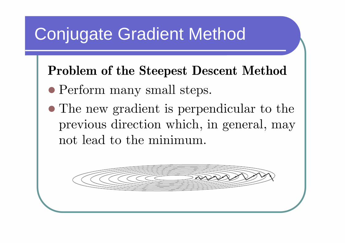
Conjugate Gradient Method
Problem of the Steepest Descent MethodPerform many small steps.The new gradient is perpendicular to the previous direction which, in general, may not lead to the minimum.

Conjugate Gradient Method
We want to proceed in a new direction that is conjugate to the old gradient as well as all previous directions. The method is called the conjugate gradientmethod.
The conjugate gradient method is an iterative method that will end in n steps, where n is the dimension of the system.

Conjugate Gradient Method
We want to construct an orthogonal set {p0, p1, …, pn–1} where
that is to say “pi is conjugate to pj”.
Since A is positive definite, we have that
T 0 for all i j i j= ≠p Ap
T 0i i >p Ap

Conjugate Gradient Method
For k = 1, ..., n, let
which satisfies the recurrence relation
We need that
is the minimum point; thus, Axn = b.
1k k k kα+ = +x x p
0 0 0 1 1 1 1k k kα α α − −= + + + +x x p p p
0 0 0 1 1 1 1n n nα α α − −= + + + +x x p p p
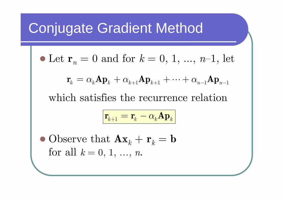
Conjugate Gradient Method
Let rn = 0 and for k = 0, 1, ..., n–1, let
which satisfies the recurrence relation
Observe that Axk + rk = bfor all k = 0, 1, …, n.
1 1 1 1k k k k k n nα α α+ + − −= + + +r Ap Ap Ap
1k k k kα+ = −r r Ap

Conjugate Gradient Method
It should be noted that
Using the conjugacy of pk’s, the coefficient αk can be found from
T
Tk k
k
k k
α =r p
p Ap
TT
0 if
if k ii k k
i k
i kα
⎧ <⎪⎪⎪= ⎨⎪ ≥⎪⎪⎩r p
p Ap

Conjugate Gradient Method
Start with p0 = r0. For each pk+1, choose a direction slightly different from rk+1, i.e.
Since ri = pi – βipi–1, we have that
which means that {r0, r1, …, rn–1} is also an orthogonal set.
1 1k k k kβ+ += +p r p
T 0 for all i j i j= ≠r r

Conjugate Gradient Method
Observe that
therefore
Notice that
therefore
T T T1 1k k k k k k kβ+ += +r p r r r p
T1 1T
k kk
k k
β + +=r rr r
( )T T T1 1k k k k k k k k
β − −= + =r p r r p r r
T
Tk k
kk k
α =r r
p Ap
T T1 1 1 0k k k k k k kα β α+ + + = +p Ap p Ap

Conjugate Gradient Method
The Conjugate Gradient Algorithm
T
1 1T
T1 1
1 1
0 0 0
T
T
if is sufficiently small the
1
n return
, ,
,
k
k k
kk k k k k k k k k
k k
k kk k k k
k
kk k
k k
α α α
β β
+ +
+ ++ +
⎧⎪⎪⎪⎪⎪⎪ = = + = −⎪⎪⎪⎪⎨⎪⎪⎪ = = +⎪⎪⎪⎪⎪⎪ =
=
⎩ +⎪
= −
r rx x p r r Ap
p Ap
r rp r p
repea
p r b Ax
r r x
r
t
r

Conjugate Gradient Method
If we do not know the Hessian matrix A, we could just use the gradient function ∇f(x).If we proceed from xk along the direction pk to the local minimum of f at a point xk+1, then
where
T1( ) 0k kf +∇ =p x
1 .k k k kα+ = +x x p

Conjugate Gradient Method
For a quadractic function
the gradient function isThe line minimization leads to
T T1( )
2f c= − +x b x x Ax
( ) .f∇ = −x Ax b
( )
( )
T
T
0
0
k k k k
k k k k
α
α
+ − =
− =
p Ax Ap b
p Ap r

Conjugate Gradient Method
We thus arrive at
as before.
Thus the algorithm does not require the Hessian matrix A, but line minimizations and the gradient vector.
T
Tk k
kk k
α =p r
p Ap

Conjugate Gradient Method
For an arbitrary function, rk is not necessarily perpendicular to rk+1. Polakand Ribiere introduced one tiny, but sometimes significant, change – the new direction pk+1 = rk+1 + βkpk should be constructed using
( )T
1 1
T
k k kk
k k
β + +−=
r r r
r r

Newton’s Method
An iterative method for solving systems of nonlinear equations.Generalize the Newton’s method for solving f(x)=0 using the general iterative formula:
1
( )( )
nn n
n
f xx x
f x+ = −′

Newton’s Method
Consider a system of two nonlinearequations:
The zero curve of f(x,y) is the intersection of the graph of z = f(x,y) in xyz-space with the xy-plane.
( , ) 0
( , ) 0
f x y
g x y
⎧ =⎪⎪⎪⎨⎪ =⎪⎪⎩

-3 -2 -1 1 2 3
-2
-1
1
2
3
Newton’s Method
An illustrating example:
2 2
2
( , ) 4 9 0
( , ) 18 14 45 0
f x y x y
g x y y x
⎧ ≡ + − =⎪⎪⎪⎨⎪ ≡ − + =⎪⎪⎩
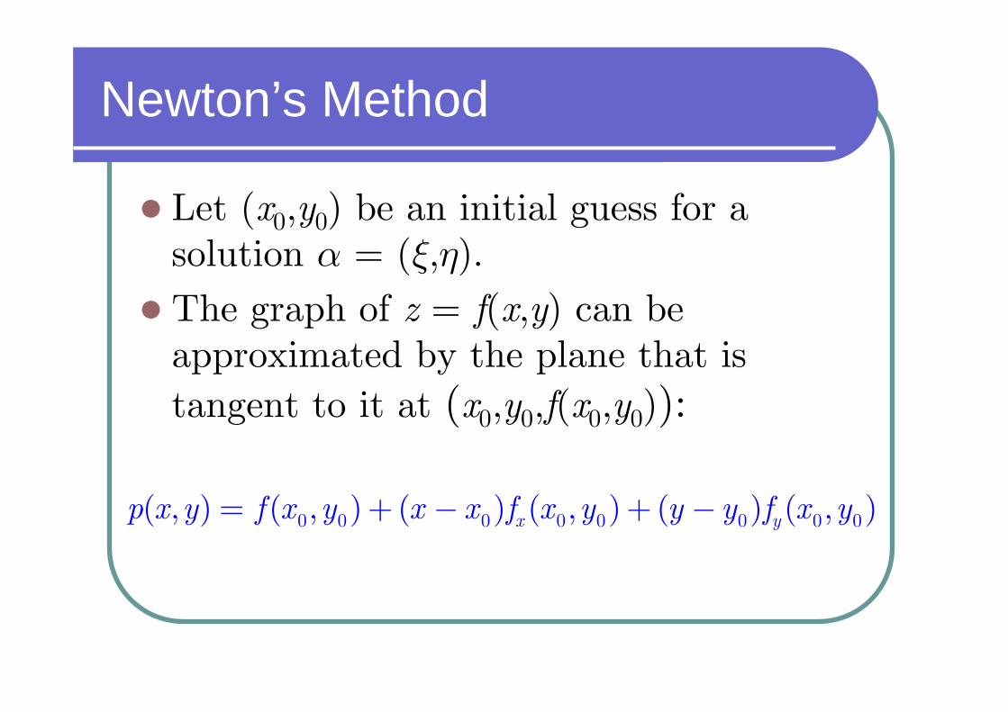
Newton’s Method
Let (x0,y0) be an initial guess for a solution α = (ξ,η).The graph of z = f(x,y) can be approximated by the plane that is tangent to it at (x0,y0,f(x0,y0)):
0 0 0 0 0 0 0 0( , ) ( , ) ( ) ( , ) ( ) ( , )x yp x y f x y x x f x y y y f x y= + − + −

-2
0
2
-2
0
20
10
20
-2
0
2
Newton’s Method
For f(x,y) = x 2 + 4y 2 – 9and (x0,y0) = (1,–1):
( , ) 4 2( 1) 8( 1)p x y x y≡ − + − − +
-3 -2 -1 1 2 3 4
-2
-1
1

-3 -2 -1 1 2 3 4
-3
-2
-1
1
2
3
Newton’s Method
Similarly, for the surface z = g(x,y), we construct the tangent plane:
0 0 0 0 0 0 0 0( , ) ( , ) ( ) ( , ) ( ) ( , )x yq x y g x y x x g x y y y g x y= + − + −

Newton’s Method
We approximate the solution α = (ξ,η) by the intersection of the planes z = p(x,y) and z = q(x,y), which can be solved from the linear system:
0 0 0 0 0 0 0
00 0 0 0 0 0
( , ) ( , ) ( , )
( , ) ( , ) ( , )
x y
x y
f x y f x y x x f x y
y yg x y g x y g x y
⎡ ⎤ ⎡ ⎤−⎡ ⎤⎢ ⎥ ⎢ ⎥⎢ ⎥ = −⎢ ⎥ ⎢ ⎥−⎢ ⎥⎢ ⎥ ⎢ ⎥⎣ ⎦⎣ ⎦ ⎣ ⎦

Newton’s Method
Let the solution of the linear system be (x1,y1), then
(x1,y1) is usually close to the solution α than is the original point (x0,y0). The process can be iterated to get even better approximation
1
1 0 0 0 0 0 0 0
1 0 0 0 0 0 0 0
( , ) ( , ) ( , )
( , ) ( , ) ( , )
x y
x y
x x f x y f x y f x y
y y g x y g x y g x y
−⎡ ⎤ ⎡ ⎤⎡ ⎤ ⎡ ⎤ ⎢ ⎥ ⎢ ⎥⎢ ⎥ ⎢ ⎥= − ⎢ ⎥ ⎢ ⎥⎢ ⎥ ⎢ ⎥ ⎢ ⎥ ⎢ ⎥⎣ ⎦ ⎣ ⎦ ⎣ ⎦ ⎣ ⎦

Newton’s Method
In general for the systemof nonlinear equations:
Introduce the symbols:
1 1 2
2 1 2
( , ) 0
( , ) 0
F x x
F x x
⎧ =⎪⎪⎪⎨⎪ =⎪⎪⎩
1
2
xx x
⎡ ⎤⎢ ⎥= ⎢ ⎥⎣ ⎦
1 1 2
2 1 2
( , )( )
( , )
F x xF x
F x x
⎡ ⎤⎢ ⎥= ⎢ ⎥⎢ ⎥⎣ ⎦
1 1
2 2
( ) ( )( )
( ) ( )
x y
x y
F FF x
F F
⎡ ⎤⎢ ⎥′ = ⎢ ⎥⎢ ⎥⎣ ⎦
Frechet Derivative

Newton’s Method
The Newton’s method for solving the nonlinear system becomes
The method can be extended to higher dimensional problems.
( ) 1( 1) ( ) ( ) ( )( ) ( )k k k kx x F x F x−+ ′= −
Newton’s Method
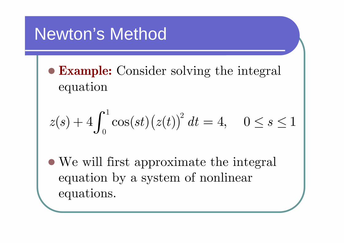
Example: Consider solving the integral equation
We will first approximate the integral equation by a system of nonlinear equations.
( )1 2
0( ) 4 cos( ) ( ) 4, 0 1z s st z t dt s+ = ≤ ≤∫

Newton’s Method
For some n > 0, let h = 1/n and
Use the midpoint numerical integration:
( )12
, 1,2, ,jt j h j n= − = …
( )1
01
( )n
jj
f t dt h f t=
≈ ∑∫
Newton’s Method
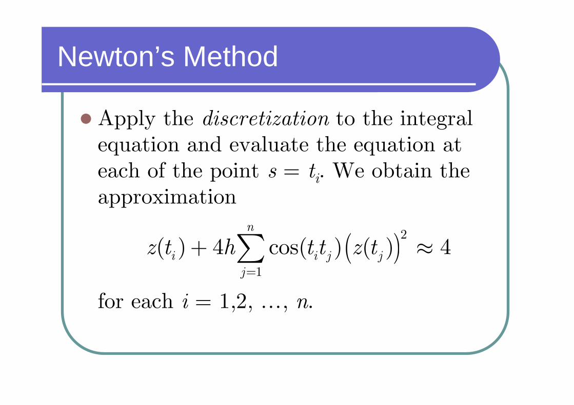
Apply the discretization to the integral equation and evaluate the equation at each of the point s = ti. We obtain the approximation
for each i = 1,2, …, n.
( )2
1
( ) 4 cos( ) ( ) 4n
i i j jj
z t h t t z t=
+ ≈∑

Newton’s Method
We can solve the system of n equations:
for i = 1,2, …, n, and hope that
for each i.
( )2
1
4 cos( ) 4n
i i j ij
x h t t x=
+ ≈∑
( )i iz t x≈


