144
CHAPTER 3 NUMERICAL DESCRIPTIVE MEASURES Prem Mann, Introductory Statistics, 8/E Copyright © 2013 John Wiley & Sons. All rights reserved.
| Date post: | 17-Dec-2015 |
| Category: |
Documents |
| Upload: | philip-parsons |
| View: | 267 times |
| Download: | 16 times |
CHAPTER 3
NUMERICAL DESCRIPTIVE MEASURES
Prem Mann, Introductory Statistics, 8/E Copyright © 2013 John Wiley & Sons. All rights reserved.

Opening Example
Prem Mann, Introductory Statistics, 8/E Copyright © 2013 John Wiley & Sons. All rights reserved.

MEASURES OF CENTRAL TENDENCY FOR UNGROUPED DATA
Mean Median Mode Relationships among the Mean, Median, and Mode
Prem Mann, Introductory Statistics, 8/E Copyright © 2013 John Wiley & Sons. All rights reserved.
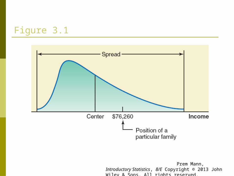
Figure 3.1
Prem Mann, Introductory Statistics, 8/E Copyright © 2013 John Wiley & Sons. All rights reserved.
Mean
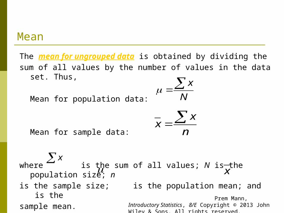
The mean for ungrouped data is obtained by dividing the sum of all values by the number of values in the data set. Thus,
Mean for population data:
Mean for sample data:
where is the sum of all values; N is the population size; n is the sample size; is the population mean; and is the sample mean.
N
x
n
xx
x
x
Prem Mann, Introductory Statistics, 8/E Copyright © 2013 John Wiley & Sons. All rights reserved.

Example 3-1
Table 3.1 lists the total cash donations (rounded to millions of dollars) given by eight U.S. companies during the year 2010 (Source: Based on U.S. Internal Revenue Service data analyzed by The Chronicle of Philanthropy and USA TODAY).
Prem Mann, Introductory Statistics, 8/E Copyright © 2013 John Wiley & Sons. All rights reserved.

Table 3.1 Cash Donations in 2010 by Eight U.S. Companies
Find the mean of cash donations made by these eight companies.
Prem Mann, Introductory Statistics, 8/E Copyright © 2013 John Wiley & Sons. All rights reserved.
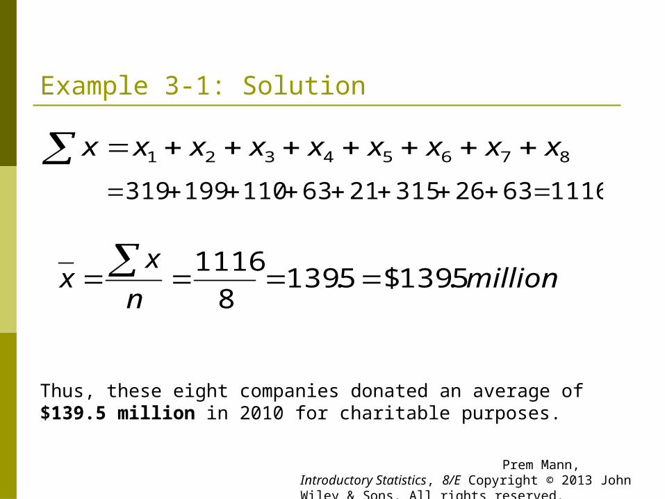
Example 3-1: Solution
Thus, these eight companies donated an average of $139.5 million in 2010 for charitable purposes.
87654321 xxxxxxxxx
millionn
xx 5.139$5.139
8
1116
111663263152163110199319
Prem Mann, Introductory Statistics, 8/E Copyright © 2013 John Wiley & Sons. All rights reserved.

Example 3-2
The following are the ages (in years) of all eight employees of a
small company:53 32 61 27 39 44 49 57
Find the mean age of these employees.
Prem Mann, Introductory Statistics, 8/E Copyright © 2013 John Wiley & Sons. All rights reserved.

Example 3-2: Solution
years 25.458
362
N
x
The population mean is
Thus, the mean age of all eight employees of this company is 45.25 years, or 45 years and 3 months.
Prem Mann, Introductory Statistics, 8/E Copyright © 2013 John Wiley & Sons. All rights reserved.

Example 3-3
Table 3.2 lists the total number of homes lost to foreclosure in seven states during 2010.
Prem Mann, Introductory Statistics, 8/E Copyright © 2013 John Wiley & Sons. All rights reserved.

Table 3.2 Number of Homes Foreclosed in 2010
Prem Mann, Introductory Statistics, 8/E Copyright © 2013 John Wiley & Sons. All rights reserved.
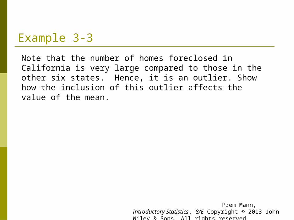
Example 3-3
Note that the number of homes foreclosed in California is very large compared to those in the other six states. Hence, it is an outlier. Show how the inclusion of this outlier affects the value of the mean.
Prem Mann, Introductory Statistics, 8/E Copyright © 2013 John Wiley & Sons. All rights reserved.

Example 3-3: Solution If we do not include the number of homes foreclosed in
California (the outlier), the mean of the number of foreclosed homes in six states is
616,336
696,2016
848,61038,18911,40824,10352,20723,49
outlier the without Mean
Prem Mann, Introductory Statistics, 8/E Copyright © 2013 John Wiley & Sons. All rights reserved.

Example 3-3: Solution
Now, to see the impact of the outlier on the value of the mean, we include the number of homes foreclosed in California and find the mean number of homes foreclosed in the seven states. This mean is
553,537
871,3746
848,61038,18911,40824,10352,20723,49175,173
outlier the withMean
Prem Mann, Introductory Statistics, 8/E Copyright © 2013 John Wiley & Sons. All rights reserved.

Case Study 3-1 Average NFL Ticket Prices in the Secondary Market
Prem Mann, Introductory Statistics, 8/E Copyright © 2013 John Wiley & Sons. All rights reserved.

Median Definition The median is the value of the middle term in a data set that
has been ranked in increasing order.
The calculation of the median consists of the following two steps:1. Rank the data set in increasing order.2. Find the middle term. The value of this term is the median.
Prem Mann, Introductory Statistics, 8/E Copyright © 2013 John Wiley & Sons. All rights reserved.
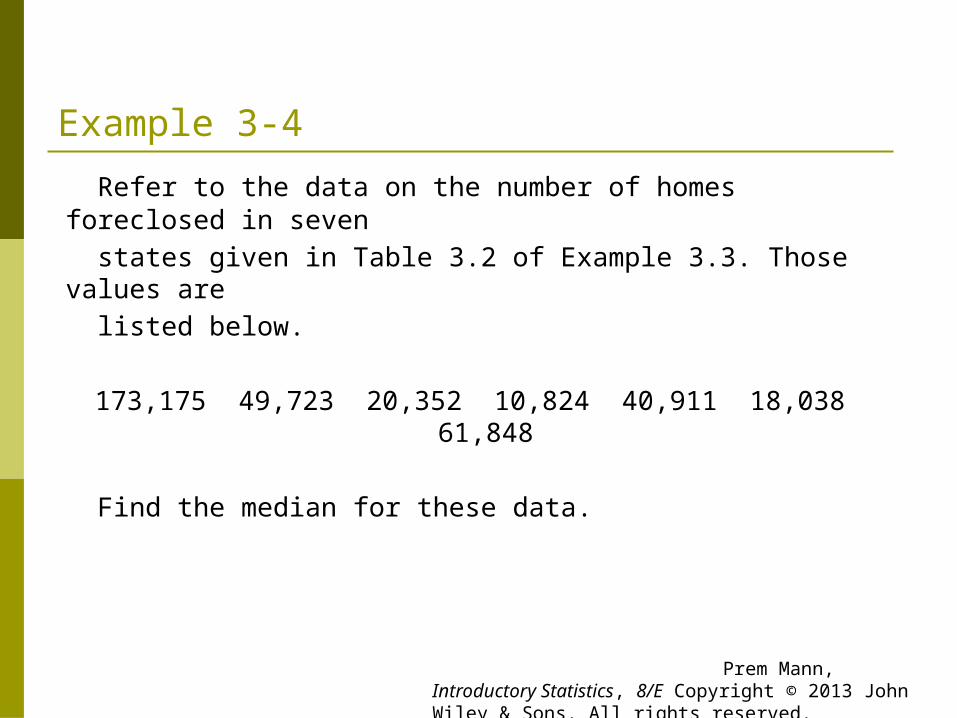
Example 3-4
Refer to the data on the number of homes foreclosed in seven states given in Table 3.2 of Example 3.3. Those values are listed below.
173,175 49,723 20,352 10,824 40,911 18,038 61,848
Find the median for these data.
Prem Mann, Introductory Statistics, 8/E Copyright © 2013 John Wiley & Sons. All rights reserved.

Example 3-4: Solution
First, we rank the given data in increasing order as follows: 10,824 18,038 20,352 40,911 49,723 61,848 173,175
Since there are seven homes in this data set and the middle
term is the fourth term,
Thus, the median number of homes foreclosed in these seven states was 40,911 in 2010.
Prem Mann, Introductory Statistics, 8/E Copyright © 2013 John Wiley & Sons. All rights reserved.

Example 3-5
Table 3.3 gives the total compensations (in millions of dollars) for the year 2010 of the 12 highest-paid CEOs of U.S. companies.
Prem Mann, Introductory Statistics, 8/E Copyright © 2013 John Wiley & Sons. All rights reserved.

Table 3.3 Total Compensations of 12 Highest-Paid CEOs for the Year 2010
Find the median for these data.
Prem Mann, Introductory Statistics, 8/E Copyright © 2013 John Wiley & Sons. All rights reserved.
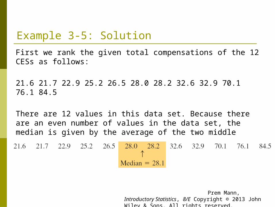
Example 3-5: Solution First we rank the given total compensations of the 12 CESs as
follows:
21.6 21.7 22.9 25.2 26.5 28.0 28.2 32.6 32.9 70.1 76.1 84.5
There are 12 values in this data set. Because there are an even number of values in the data set, the median is given by the average of the two middle values.
Prem Mann, Introductory Statistics, 8/E Copyright © 2013 John Wiley & Sons. All rights reserved.

Example 3-5: Solution The two middle values are the sixth and seventh in the
arranged data, and these two values are 28.0 and 28.2.
Thus, the median for the 2010 compensations of these 12 CEOs is $28.1 million.
million1.28$1.282
2.56
2
2.280.28 Median
Prem Mann, Introductory Statistics, 8/E Copyright © 2013 John Wiley & Sons. All rights reserved.
Median
The median gives the center of a histogram, with half the data values to the left of the median and half to the right of the median. The advantage of using the median as a measure of central tendency is that it is not influenced by outliers. Consequently, the median is preferred over the mean as a measure of central tendency for data sets that contain outliers.
Prem Mann, Introductory Statistics, 8/E Copyright © 2013 John Wiley & Sons. All rights reserved.

Case Study 3-3 Education Pays
Prem Mann, Introductory Statistics, 8/E Copyright © 2013 John Wiley & Sons. All rights reserved.
Mode Definition The mode is the value that occurs with the highest frequency
in a data set.
Prem Mann, Introductory Statistics, 8/E Copyright © 2013 John Wiley & Sons. All rights reserved.

Example 3-6 The following data give the speeds (in miles per hour) of eight
cars that were stopped on I-95 for speeding violations.
77 82 74 81 79 84 74 78
Find the mode.
Prem Mann, Introductory Statistics, 8/E Copyright © 2013 John Wiley & Sons. All rights reserved.
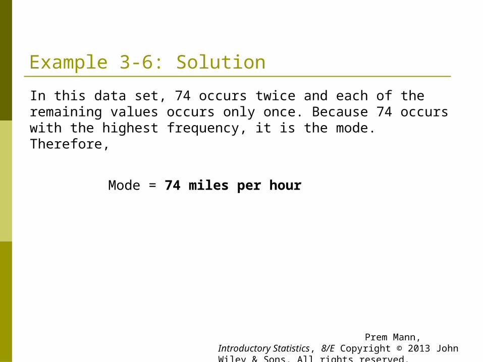
Example 3-6: Solution
In this data set, 74 occurs twice and each of the remaining values occurs only once. Because 74 occurs with the highest frequency, it is the mode. Therefore,
Mode = 74 miles per hour
Prem Mann, Introductory Statistics, 8/E Copyright © 2013 John Wiley & Sons. All rights reserved.
Mode A major shortcoming of the mode is that a data set may
have none or may have more than one mode, whereas it will have only one mean and only one median. Unimodal: A data set with only one mode. Bimodal: A data set with two modes. Multimodal: A data set with more than two modes.
Prem Mann, Introductory Statistics, 8/E Copyright © 2013 John Wiley & Sons. All rights reserved.
Example 3-7 (Data set with no mode) Last year’s incomes of five randomly selected families were
$76,150, $95,750, $124,985, $87,490, and $53,740.
Find the mode.
Prem Mann, Introductory Statistics, 8/E Copyright © 2013 John Wiley & Sons. All rights reserved.

Example 3-7: Solution Because each value in this data set occurs only once, this data
set contains no mode.
Prem Mann, Introductory Statistics, 8/E Copyright © 2013 John Wiley & Sons. All rights reserved.
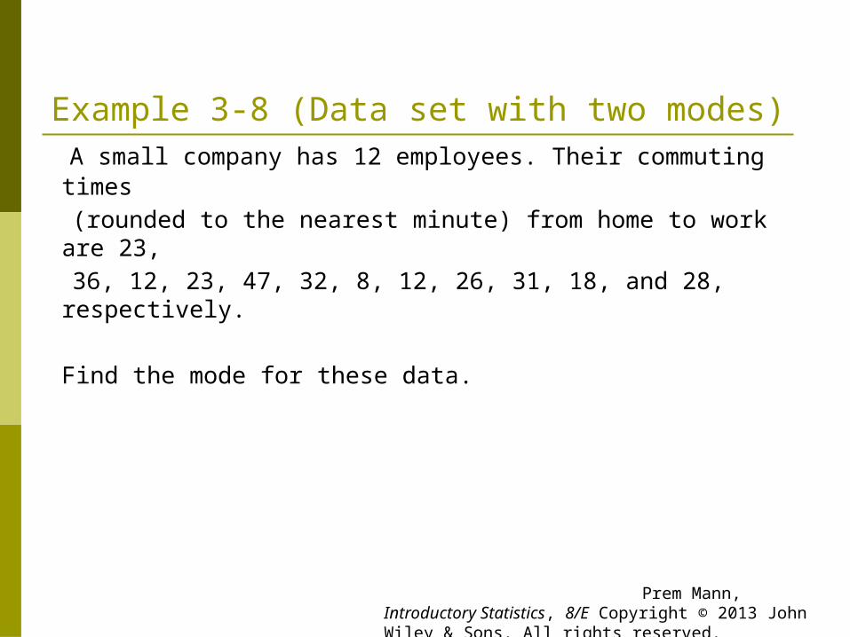
Example 3-8 (Data set with two modes) A small company has 12 employees. Their commuting times
(rounded to the nearest minute) from home to work are 23, 36, 12, 23, 47, 32, 8, 12, 26, 31, 18, and 28, respectively.
Find the mode for these data.
Prem Mann, Introductory Statistics, 8/E Copyright © 2013 John Wiley & Sons. All rights reserved.

Example 3-8: Solution
In the given data on the commuting times of the 12 employees, each of the values 12 and 23 occurs twice, and each of the remaining values occurs only once. Therefore, that data set has two modes: 12 and 23 minutes.
Prem Mann, Introductory Statistics, 8/E Copyright © 2013 John Wiley & Sons. All rights reserved.

Example 3-9 (Data set with three modes)
The ages of 10 randomly selected students from a class are 21, 19, 27, 22, 29, 19, 25, 21, 22 and 30 years, respectively.
Find the mode.
Prem Mann, Introductory Statistics, 8/E Copyright © 2013 John Wiley & Sons. All rights reserved.
Example 3-9: Solution
This data set has three modes: 19, 21 and 22. Each of these three values occurs with a (highest) frequency of 2.
Prem Mann, Introductory Statistics, 8/E Copyright © 2013 John Wiley & Sons. All rights reserved.

Mode
One advantage of the mode is that it can be calculated for both kinds of data - quantitative and qualitative - whereas the mean and median can be calculated for only quantitative data.
Prem Mann, Introductory Statistics, 8/E Copyright © 2013 John Wiley & Sons. All rights reserved.

Example 3-10
The status of five students who are members of the student senate at a college are senior, sophomore, senior, junior, and senior, respectively. Find the mode.
Prem Mann, Introductory Statistics, 8/E Copyright © 2013 John Wiley & Sons. All rights reserved.
Example 3-10: Solution Because senior occurs more frequently than the other
categories, it is the mode for this data set. We cannot calculate the mean and median for this data set.
Prem Mann, Introductory Statistics, 8/E Copyright © 2013 John Wiley & Sons. All rights reserved.

Relationships Among the Mean, Median, and Mode
1. For a symmetric histogram and frequency distribution with one peak (see Figure 3.2), the values of the mean, median, and mode are identical, and they lie at the center of the distribution.
Prem Mann, Introductory Statistics, 8/E Copyright © 2013 John Wiley & Sons. All rights reserved.

Figure 3.2 Mean, median, and mode for a symmetric histogram and frequency distribution curve.
Prem Mann, Introductory Statistics, 8/E Copyright © 2013 John Wiley & Sons. All rights reserved.

Relationships Among the Mean, Median, and Mode2. For a histogram and a frequency distribution curve skewed
to the right (see Figure 3.3), the value of the mean is the largest, that of the mode is the smallest, and the value of the median lies between these two. (Notice that the mode always occurs at the peak point.) The value of the mean is the largest in this case because it is sensitive to outliers that occur in the right tail. These outliers pull the mean to the right.
Prem Mann, Introductory Statistics, 8/E Copyright © 2013 John Wiley & Sons. All rights reserved.

Figure 3.3 Mean, median, and mode for a histogram and frequency distribution curve skewed to the right.
Prem Mann, Introductory Statistics, 8/E Copyright © 2013 John Wiley & Sons. All rights reserved.
Relationships Among the Mean, Median, and Mode
3. If a histogram and a frequency distribution curve are skewed to the left (see Figure 3.4), the value of the mean is the smallest and that of the mode is the largest, with the value of the median lying between these two. In this case, the outliers in the left tail pull the mean to the left.
Prem Mann, Introductory Statistics, 8/E Copyright © 2013 John Wiley & Sons. All rights reserved.

Figure 3.4 Mean, median, and mode for a histogram and frequency distribution curve skewed to the left.
Prem Mann, Introductory Statistics, 8/E Copyright © 2013 John Wiley & Sons. All rights reserved.
MEASURES OF DISPERSION FOR UNGROUPED DATA
Range Variance and Standard Deviation Population Parameters and Sample Statistics
Prem Mann, Introductory Statistics, 8/E Copyright © 2013 John Wiley & Sons. All rights reserved.
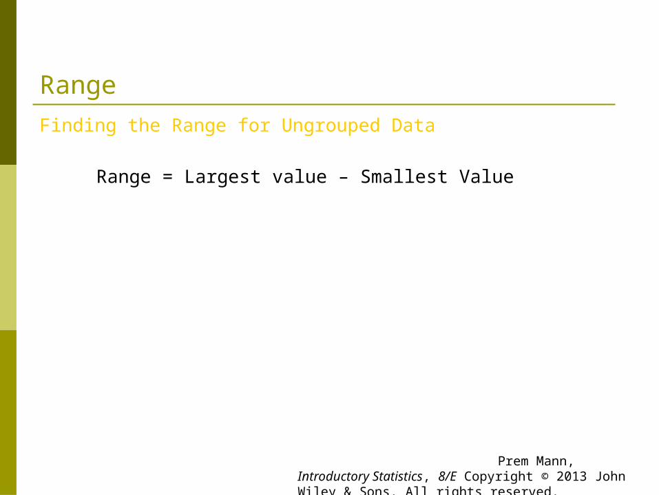
Range
Finding the Range for Ungrouped Data
Range = Largest value – Smallest Value
Prem Mann, Introductory Statistics, 8/E Copyright © 2013 John Wiley & Sons. All rights reserved.
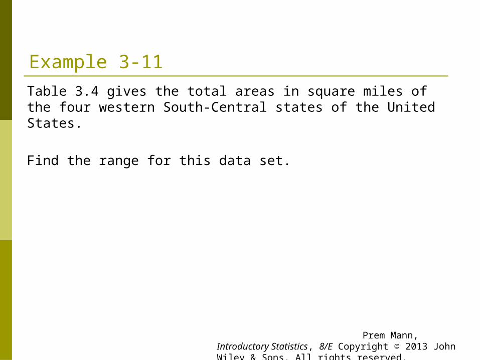
Example 3-11 Table 3.4 gives the total areas in square miles of the four
western South-Central states of the United States.
Find the range for this data set.
Prem Mann, Introductory Statistics, 8/E Copyright © 2013 John Wiley & Sons. All rights reserved.
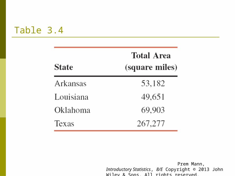
Table 3.4
Prem Mann, Introductory Statistics, 8/E Copyright © 2013 John Wiley & Sons. All rights reserved.

Example 3-11: Solution
Range = Largest value – Smallest Value = 267,277 – 49,651 = 217,626 square miles
Thus, the total areas of these four states are spread over a range of
217,626 square miles.
Prem Mann, Introductory Statistics, 8/E Copyright © 2013 John Wiley & Sons. All rights reserved.
Range
Disadvantages The range, like the mean, has the disadvantage of being
influenced by outliers. Consequently, the range is not a good measure of dispersion to use for a data set that contains outliers.
Its calculation is based on two values only: the largest and the smallest. All other values in a data set are ignored when calculating the range. Thus, the range is not a very satisfactory measure of dispersion.
Prem Mann, Introductory Statistics, 8/E Copyright © 2013 John Wiley & Sons. All rights reserved.

Variance and Standard Deviation The standard deviation is the most-used measure of
dispersion.
The value of the standard deviation tells how closely the values of a data set are clustered around the mean.
In general, a lower value of the standard deviation for a data set indicates that the values of that data set are spread over a relatively smaller range around the mean.
Prem Mann, Introductory Statistics, 8/E Copyright © 2013 John Wiley & Sons. All rights reserved.

Variance and Standard Deviation In contrast, a larger value of the standard deviation for a
data set indicates that the values of that data set are spread over a relatively larger range around the mean.
The standard deviation is obtained by taking the positive square root of the variance.
Prem Mann, Introductory Statistics, 8/E Copyright © 2013 John Wiley & Sons. All rights reserved.

Variance and Standard Deviation The variance calculated for population data is denoted by σ²
(read as sigma squared), and the variance calculated for sample data is denoted by s².
The standard deviation calculated for population data is denoted by σ, and the standard deviation calculated for sample data is denoted by s.
Consequently, the standard deviation calculated for population data is denoted by σ, and the standard deviation calculated for sample data is denoted by s.
Prem Mann, Introductory Statistics, 8/E Copyright © 2013 John Wiley & Sons. All rights reserved.

Variance and Standard Deviation Basic Formulas for the Variance and Standard Deviation for
Ungrouped Data
where σ² is the population variance, s² is the sample variance, σ is the population standard deviation, and s is the sample standard deviation.
1
and
1 and
22
2
22
2
n
xxs
N
x
n
xxs
N
x
Prem Mann, Introductory Statistics, 8/E Copyright © 2013 John Wiley & Sons. All rights reserved.

Table 3.5
Prem Mann, Introductory Statistics, 8/E Copyright © 2013 John Wiley & Sons. All rights reserved.
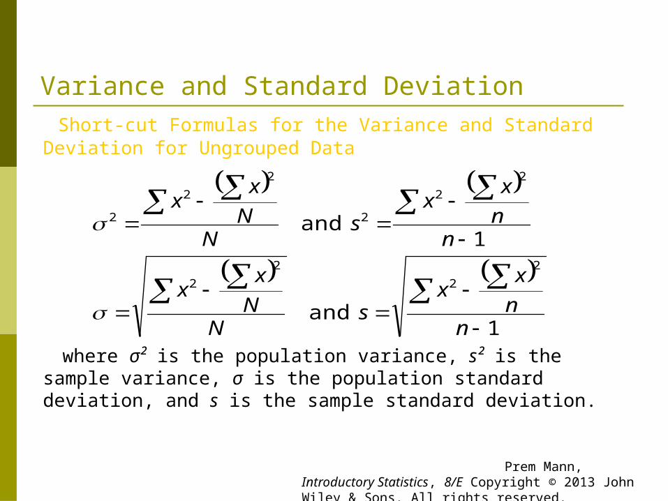
Variance and Standard Deviation Short-cut Formulas for the Variance and Standard Deviation
for Ungrouped Data
where σ² is the population variance, s² is the sample variance, σ is the population standard deviation, and s is the sample standard deviation.
1 and
1 and
2
2
2
2
2
2
2
2
2
2
nn
xx
sN
N
xx
nn
xx
sN
N
xx
Prem Mann, Introductory Statistics, 8/E Copyright © 2013 John Wiley & Sons. All rights reserved.

Example 3-12
Until about 2009, airline passengers were not charged for checked baggage. Around 2009, however, many U.S. airlines started charging a fee for bags. According to the Bureau of Transportation Statistics, U.S. airlines collected more than $3 billion in baggage fee revenue in 2010. The following table lists the baggage fee revenues of six U.S. airlines for the year 2010. (Note that Delta’s revenue reflects a merger with Northwest. Also note that since then United and Continental have merged; and American filed for bankruptcy and may merge with another airline.)
Find the variance and standard deviation for these data.
Prem Mann, Introductory Statistics, 8/E Copyright © 2013 John Wiley & Sons. All rights reserved.

Example 3-12
Prem Mann, Introductory Statistics, 8/E Copyright © 2013 John Wiley & Sons. All rights reserved.

Example 3-12: SolutionLet x denote the 2010 baggage fee revenue (in millions of dollars) of an airline. The values of Σx and Σx2 are calculated in Table 3.6.
Prem Mann, Introductory Statistics, 8/E Copyright © 2013 John Wiley & Sons. All rights reserved.

Example 3-12: Solution
Step 1. Calculate Σx
The sum of values in the first column of Table 3.6 gives 2,854.
Step 2. Find Σx2
The results of this step are shown in the second column of Table 3.6, which is 1,746,098.
Prem Mann, Introductory Statistics, 8/E Copyright © 2013 John Wiley & Sons. All rights reserved.
Example 3-12: Solution
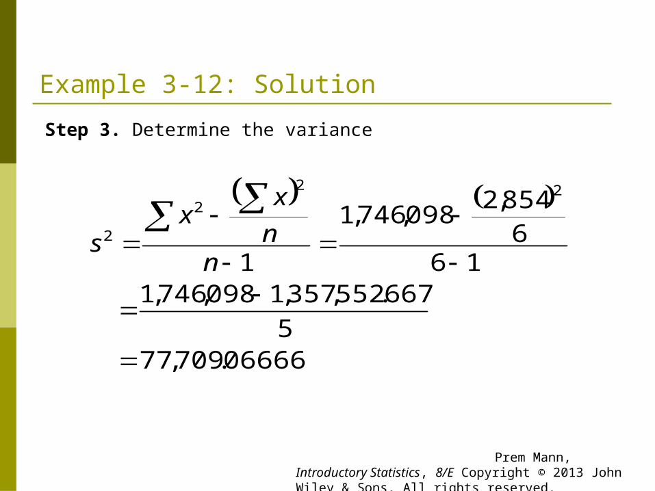
Step 3. Determine the variance
06666.709,77 5
667.552,357,1098,746,1
166
854,2098,746,1
1
22
2
2
nn
xx
s
Prem Mann, Introductory Statistics, 8/E Copyright © 2013 John Wiley & Sons. All rights reserved.

Example 3-12: Solution
Step 4. Obtain the standard deviation
The standard deviation is obtained by taking the (positive) square root of the variance:
Thus, the standard deviation of the 2010 baggage fee revenues of these six airlines is $278.76 million.
millionn
n
xx
s
76.278$7634601.278
06666.709,771
2
2
Prem Mann, Introductory Statistics, 8/E Copyright © 2013 John Wiley & Sons. All rights reserved.
Two Observations
1. The values of the variance and the standard deviation are never negative.
2. The measurement units of variance are always the square of the measurement units of the original data.
Prem Mann, Introductory Statistics, 8/E Copyright © 2013 John Wiley & Sons. All rights reserved.

Example 3-13
Following are the 2011 earnings (in thousands of dollars) before taxes for all six employees of a small company.
88.50 108.40 65.50 52.50 79.80 54.60
Calculate the variance and standard deviation for these data.
Prem Mann, Introductory Statistics, 8/E Copyright © 2013 John Wiley & Sons. All rights reserved.

Example 3-13: SolutionLet x denote the 2011 earnings before taxes of an employee of this company. The values of ∑x and ∑x2 are calculated in Table 3.7.
Prem Mann, Introductory Statistics, 8/E Copyright © 2013 John Wiley & Sons. All rights reserved.
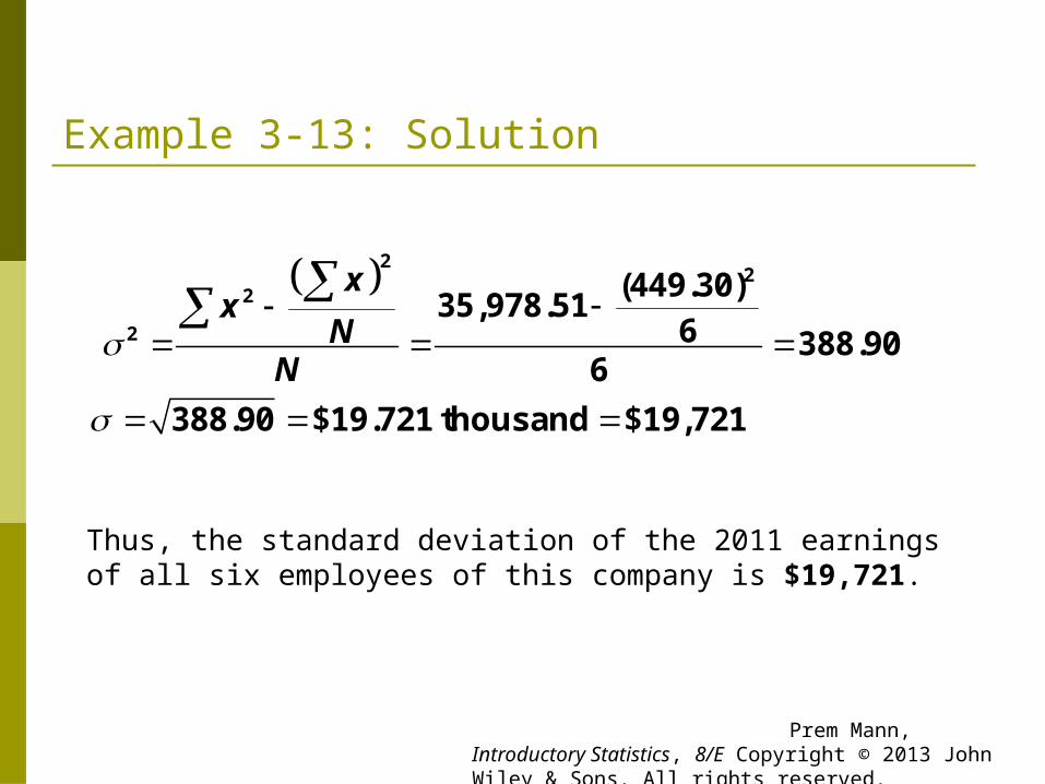
Example 3-13: Solution
22
2
2
(449.30)35,978.51
6 388.906
388.90 $19.721 thousand $19,721
xx
NN
Thus, the standard deviation of the 2011 earnings of all six employees of this company is $19,721.
Prem Mann, Introductory Statistics, 8/E Copyright © 2013 John Wiley & Sons. All rights reserved.

WarningNote that ∑x2 is not the same as (∑x)2. The value of ∑x2 is obtained by squaring the x values and then adding them. The value of (∑x)2 is obtained by squaring the value of ∑x.
Prem Mann, Introductory Statistics, 8/E Copyright © 2013 John Wiley & Sons. All rights reserved.
Population Parameters and Sample Statistics A numerical measure such as the mean, median, mode,
range, variance, or standard deviation calculated for a population data set is called a population parameter, or simply a parameter.
A summary measure calculated for a sample data set is called a sample statistic, or simply a statistic.
Prem Mann, Introductory Statistics, 8/E Copyright © 2013 John Wiley & Sons. All rights reserved.

MEAN, VARIANCE AND STANDARD DEVIATION FOR GROUPED DATA Mean for Grouped Data Variance and Standard Deviation for Grouped Data
Prem Mann, Introductory Statistics, 8/E Copyright © 2013 John Wiley & Sons. All rights reserved.

Calculating Mean for Grouped Data
Mean for population data:
Mean for sample data:
where m is the midpoint and f is the frequency of a class.
Mean for Grouped Data
N
mf
n
mfx
Prem Mann, Introductory Statistics, 8/E Copyright © 2013 John Wiley & Sons. All rights reserved.
Example 3-14
Table 3.8 gives the frequency distribution of the daily commuting times (in minutes) from home to work for all 25 employees of a company.
Calculate the mean of the daily commuting times.
Prem Mann, Introductory Statistics, 8/E Copyright © 2013 John Wiley & Sons. All rights reserved.

Example 3-14
Prem Mann, Introductory Statistics, 8/E Copyright © 2013 John Wiley & Sons. All rights reserved.
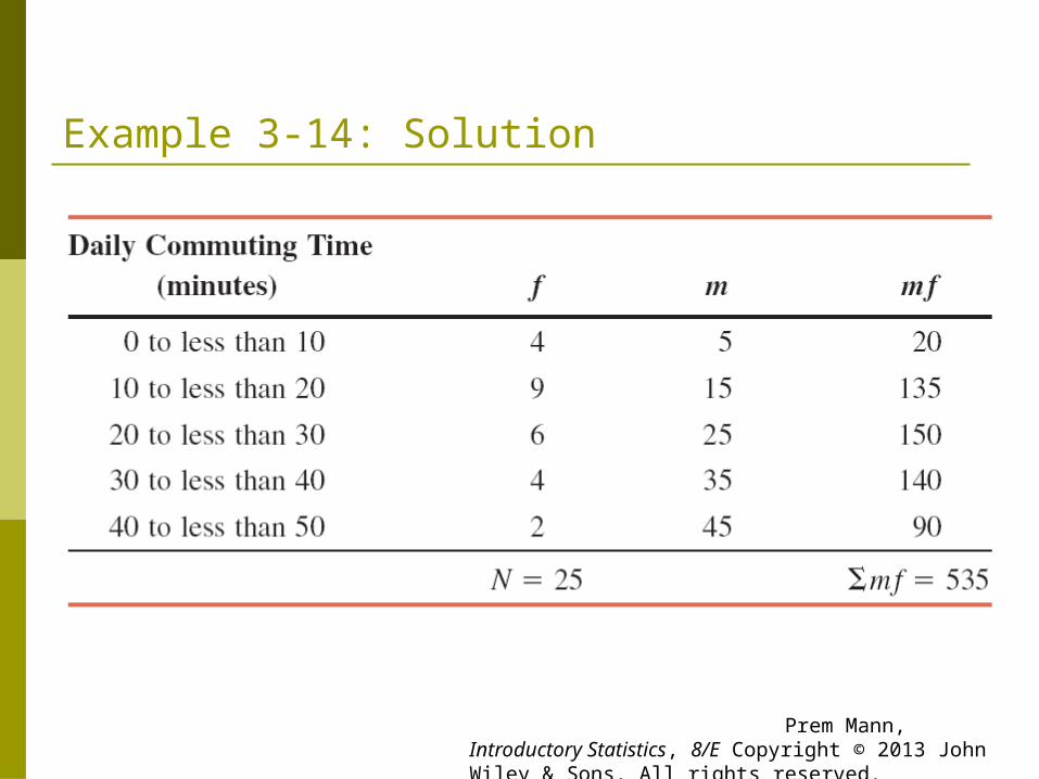
Example 3-14: Solution
Prem Mann, Introductory Statistics, 8/E Copyright © 2013 John Wiley & Sons. All rights reserved.

Example 3-14: Solution
minutes 21.4025
535
N
mf
Thus, the employees of this company spend an average of 21.40 minutes a day commuting from home to work.
Prem Mann, Introductory Statistics, 8/E Copyright © 2013 John Wiley & Sons. All rights reserved.

Example 3-15
Table 3.10 gives the frequency distribution of the number of orders received each day during the past 50 days at the office of a mail-order company.
Calculate the mean.
Prem Mann, Introductory Statistics, 8/E Copyright © 2013 John Wiley & Sons. All rights reserved.

Example 3-15
Prem Mann, Introductory Statistics, 8/E Copyright © 2013 John Wiley & Sons. All rights reserved.

Example 3-15: Solution
Prem Mann, Introductory Statistics, 8/E Copyright © 2013 John Wiley & Sons. All rights reserved.

Example 3-15: Solution
orders 16.6450
832
n
mfx
Thus, this mail-order company received an average of 16.64 orders per day during these 50 days.
Prem Mann, Introductory Statistics, 8/E Copyright © 2013 John Wiley & Sons. All rights reserved.

Variance and Standard Deviation for Grouped Data
Basic Formulas for the Variance and Standard Deviation for Grouped Data
where σ² is the population variance, s² is the sample variance, and m is the midpoint of a class. In either case, the standard deviation is obtained by taking the positive square root of the variance.
1
2
22
2
n
xmfs
N
mf and
Prem Mann, Introductory Statistics, 8/E Copyright © 2013 John Wiley & Sons. All rights reserved.

Variance and Standard Deviation for Grouped Data
Short-Cut Formulas for the Variance and Standard Deviation for Grouped Data
where σ² is the population variance, s² is the sample variance, and m is the midpoint of a class.
1
)(2
2
2
22
2
nn
mffm
sN
N
mffm
and
Prem Mann, Introductory Statistics, 8/E Copyright © 2013 John Wiley & Sons. All rights reserved.
Variance and Standard Deviation for Grouped Data
Short-cut Formulas for the Variance and Standard Deviation for
Grouped Data
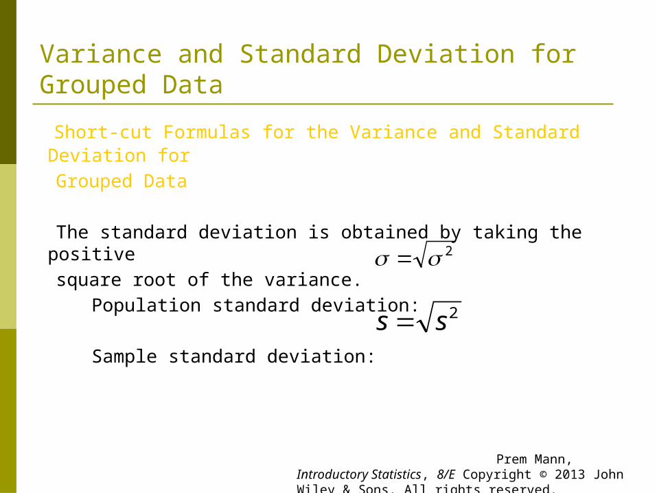
The standard deviation is obtained by taking the positive square root of the variance.
Population standard deviation:
Sample standard deviation: 2ss
2
Prem Mann, Introductory Statistics, 8/E Copyright © 2013 John Wiley & Sons. All rights reserved.

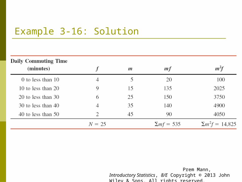
Example 3-16
The following data, reproduced from Table 3.8 of Example 3-14, give the frequency distribution of the daily commuting times (in minutes) from home to work for all 25 employees of a company.
Calculate the variance and standard deviation.
Prem Mann, Introductory Statistics, 8/E Copyright © 2013 John Wiley & Sons. All rights reserved.

Example 3-16
Prem Mann, Introductory Statistics, 8/E Copyright © 2013 John Wiley & Sons. All rights reserved.
Example 3-16: Solution
Prem Mann, Introductory Statistics, 8/E Copyright © 2013 John Wiley & Sons. All rights reserved.

Example 3-16: Solution
minutes 62.1104.135
04.13525
3376
2525
)535(825,14
)(
2
222
2
N
N
mffm
Thus, the standard deviation of the daily commuting times for these employees is 11.62 minutes.
Prem Mann, Introductory Statistics, 8/E Copyright © 2013 John Wiley & Sons. All rights reserved.
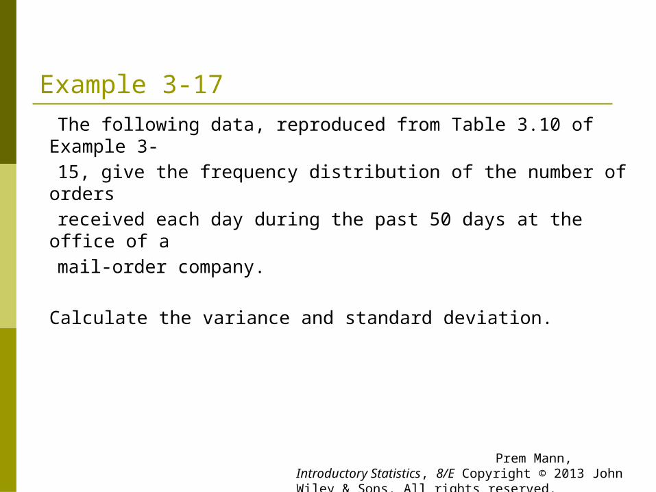
Example 3-17
The following data, reproduced from Table 3.10 of Example 3- 15, give the frequency distribution of the number of orders received each day during the past 50 days at the office of a mail-order company.
Calculate the variance and standard deviation.
Prem Mann, Introductory Statistics, 8/E Copyright © 2013 John Wiley & Sons. All rights reserved.

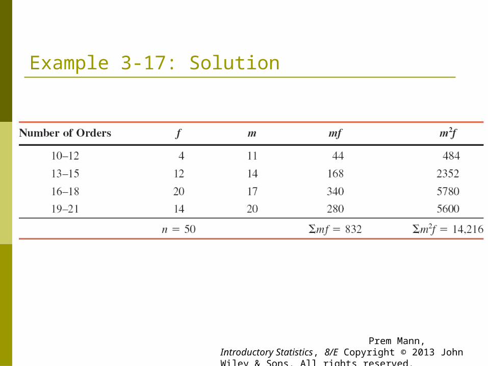
Example 3-17
Prem Mann, Introductory Statistics, 8/E Copyright © 2013 John Wiley & Sons. All rights reserved.
Example 3-17: Solution
Prem Mann, Introductory Statistics, 8/E Copyright © 2013 John Wiley & Sons. All rights reserved.

Example 3-17: Solution
orders 75.25820.7
5820.7150
50)832(
216,14
1
)(
2
222
2
ss
nn
mffm
s
Thus, the standard deviation of the number of orders received at the office of this mail-order company during the past 50 days is 2.75.
Prem Mann, Introductory Statistics, 8/E Copyright © 2013 John Wiley & Sons. All rights reserved.

USE OF STANDARD DEVIATION Chebyshev’s Theorem Empirical Rule
Prem Mann, Introductory Statistics, 8/E Copyright © 2013 John Wiley & Sons. All rights reserved.

Chebyshev’s Theorem Definition For any number k greater than 1, at least (1 – 1/k²) of the data
values lie within k standard deviations of the mean.
Prem Mann, Introductory Statistics, 8/E Copyright © 2013 John Wiley & Sons. All rights reserved.

Figure 3.5 Chebyshev’s theorem.
Prem Mann, Introductory Statistics, 8/E Copyright © 2013 John Wiley & Sons. All rights reserved.
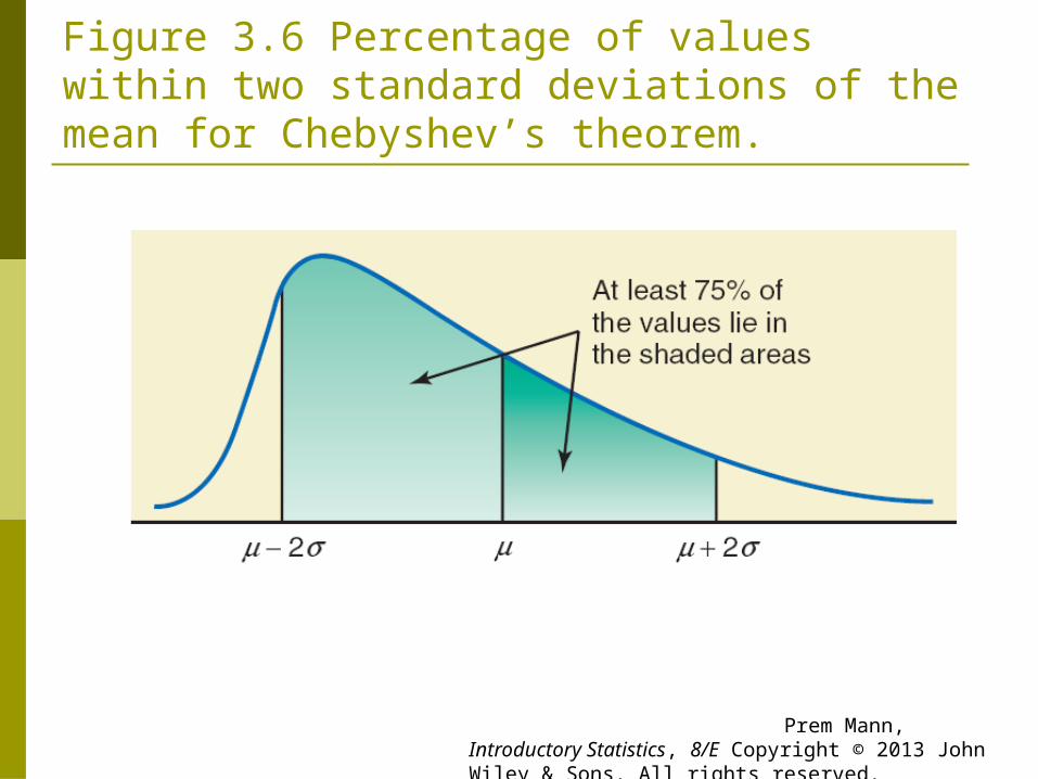
Figure 3.6 Percentage of values within two standard deviations of the mean for Chebyshev’s theorem.
Prem Mann, Introductory Statistics, 8/E Copyright © 2013 John Wiley & Sons. All rights reserved.

Figure 3.7 Percentage of values within three standard deviations of the mean for Chebyshev’s theorem.
Prem Mann, Introductory Statistics, 8/E Copyright © 2013 John Wiley & Sons. All rights reserved.
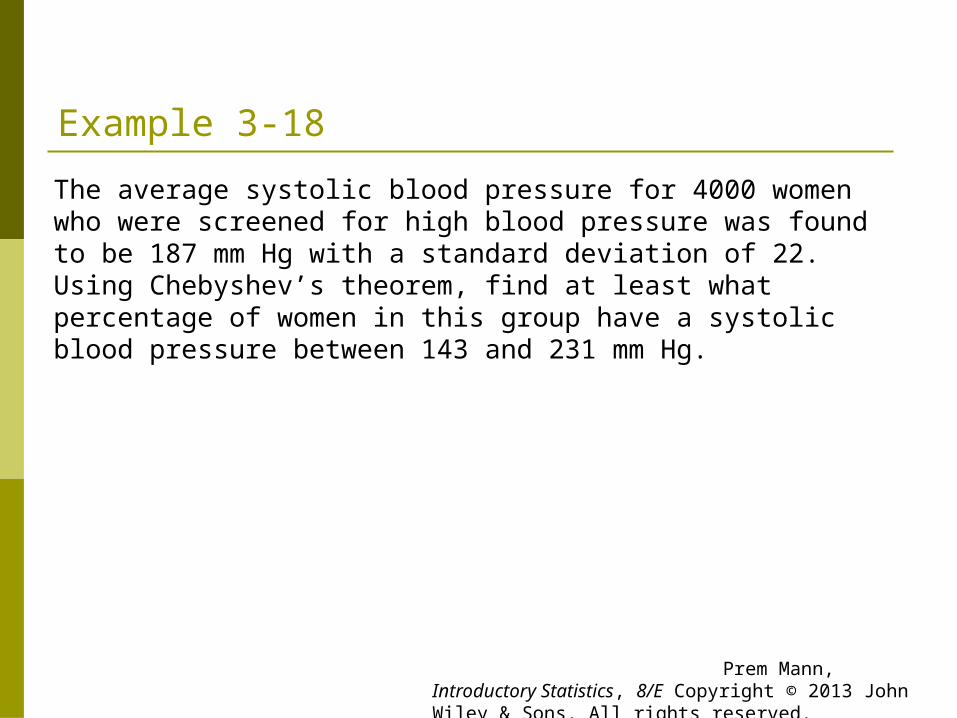
Example 3-18
The average systolic blood pressure for 4000 women who were screened for high blood pressure was found to be 187 mm Hg with a standard deviation of 22. Using Chebyshev’s theorem, find at least what percentage of women in this group have a systolic blood pressure between 143 and 231 mm Hg.
Prem Mann, Introductory Statistics, 8/E Copyright © 2013 John Wiley & Sons. All rights reserved.

Example 3-18: Solution Let μ and σ be the mean and the standard deviation,
respectively, of the systolic blood pressures of these women. μ = 187 and σ = 22
Prem Mann, Introductory Statistics, 8/E Copyright © 2013 John Wiley & Sons. All rights reserved.

Example 3-18: Solution The value of k is obtained by dividing the distance between
the mean and each point by the standard deviation. Thus k = 44/22 = 2
Hence, according to Chebyshev's theorem, at least 75% of the women have systolic blood pressure between 143 and 231 mm Hg. This percentage is shown in Figure 3.8.
75%or 75.25.14
11
)2(
11
11
22
k
Prem Mann, Introductory Statistics, 8/E Copyright © 2013 John Wiley & Sons. All rights reserved.
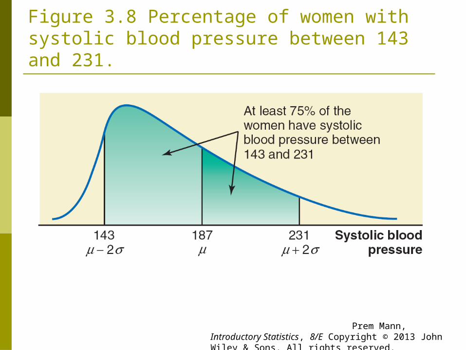
Figure 3.8 Percentage of women with systolic blood pressure between 143 and 231.
Prem Mann, Introductory Statistics, 8/E Copyright © 2013 John Wiley & Sons. All rights reserved.

Empirical Rule For a bell shaped distribution, approximately
1. 68% of the observations lie within one standard deviation of the mean
2. 95% of the observations lie within two standard deviations of the mean
3. 99.7% of the observations lie within three standard deviations of the mean
Prem Mann, Introductory Statistics, 8/E Copyright © 2013 John Wiley & Sons. All rights reserved.
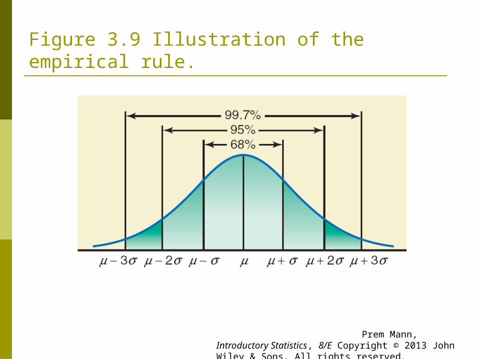
Figure 3.9 Illustration of the empirical rule.
Prem Mann, Introductory Statistics, 8/E Copyright © 2013 John Wiley & Sons. All rights reserved.
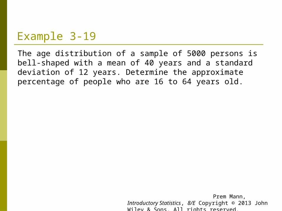
Example 3-19 The age distribution of a sample of 5000 persons is bell-shaped
with a mean of 40 years and a standard deviation of 12 years. Determine the approximate percentage of people who are 16 to 64 years old.
Prem Mann, Introductory Statistics, 8/E Copyright © 2013 John Wiley & Sons. All rights reserved.

Example 3-19: Solution From the given information, for this distribution, x = 40 and s = 12 years
Each of the two points, 16 and 64, is 24 units away from the mean.
Because the area within two standard deviations of the mean is approximately 95% for a bell-shaped curve, approximately 95% of the people in the sample are 16 to 64 years old.
Prem Mann, Introductory Statistics, 8/E Copyright © 2013 John Wiley & Sons. All rights reserved.
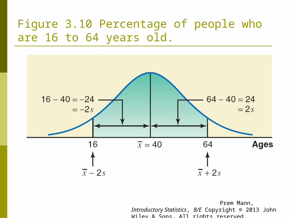
Figure 3.10 Percentage of people who are 16 to 64 years old.
Prem Mann, Introductory Statistics, 8/E Copyright © 2013 John Wiley & Sons. All rights reserved.
MEASURES OF POSITION Quartiles and Interquartile Range Percentiles and Percentile Rank
Prem Mann, Introductory Statistics, 8/E Copyright © 2013 John Wiley & Sons. All rights reserved.

Quartiles and Interquartile Range Definition Quartiles are three summary measures that divide a ranked
data set into four equal parts. The second quartile is the same as the median of a data set. The first quartile is the value of the middle term among the observations that are less than the median, and the third quartile is the value of the middle term among the observations that are greater than the median.
Prem Mann, Introductory Statistics, 8/E Copyright © 2013 John Wiley & Sons. All rights reserved.

Figure 3.11 Quartiles.
Prem Mann, Introductory Statistics, 8/E Copyright © 2013 John Wiley & Sons. All rights reserved.

Quartiles and Interquartile Range Calculating Interquartile Range The difference between the third and the first quartiles gives
the interquartile range; that is,
IQR = Interquartile range = Q3 – Q1
Prem Mann, Introductory Statistics, 8/E Copyright © 2013 John Wiley & Sons. All rights reserved.
Example 3-20
Table 3.3 in Example 3-5 gave the total compensations (in millions of dollars) for the year 2010 of the 12 highest-paid CEOs of U.S. companies. That table is reproduced on the next slide. (a) Find the values of the three quartiles. Where does the total compensation of Michael D. White (CEO of DirecTV) fall in relation to these quartiles?
(b) Find the interquartile range.
Prem Mann, Introductory Statistics, 8/E Copyright © 2013 John Wiley & Sons. All rights reserved.

Example 3-20
Prem Mann, Introductory Statistics, 8/E Copyright © 2013 John Wiley & Sons. All rights reserved.

Example 3-20: Solution
(a)
By looking at the position of $32.9 million (total compensation of Michael D. White, CEO of DirecTV), we can state that this value lies in the bottom 75% of the 2010 total compensation. This value falls between the second and third quartiles.
Prem Mann, Introductory Statistics, 8/E Copyright © 2013 John Wiley & Sons. All rights reserved.
Example 3-20: Solution
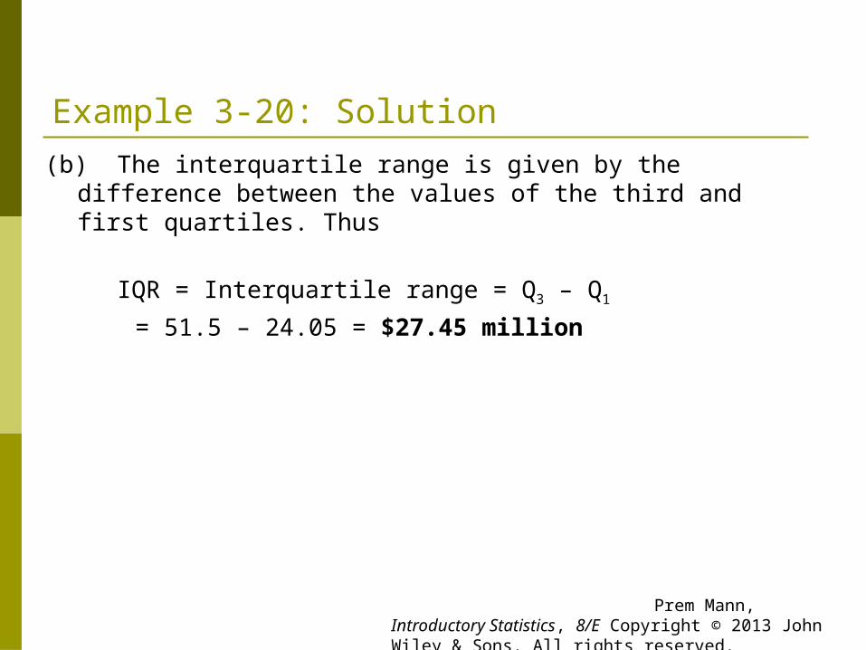
(b) The interquartile range is given by the difference between the values of the third and first quartiles. Thus
IQR = Interquartile range = Q3 – Q1
= 51.5 – 24.05 = $27.45 million
Prem Mann, Introductory Statistics, 8/E Copyright © 2013 John Wiley & Sons. All rights reserved.

Example 3-21
The following are the ages (in years) of nine employees of an insurance company: 47 28 39 51 33 37 59 24 33
(a) Find the values of the three quartiles. Where does the age of 28 years fall in relation to the ages of the employees?
(b) Find the interquartile range.
Prem Mann, Introductory Statistics, 8/E Copyright © 2013 John Wiley & Sons. All rights reserved.
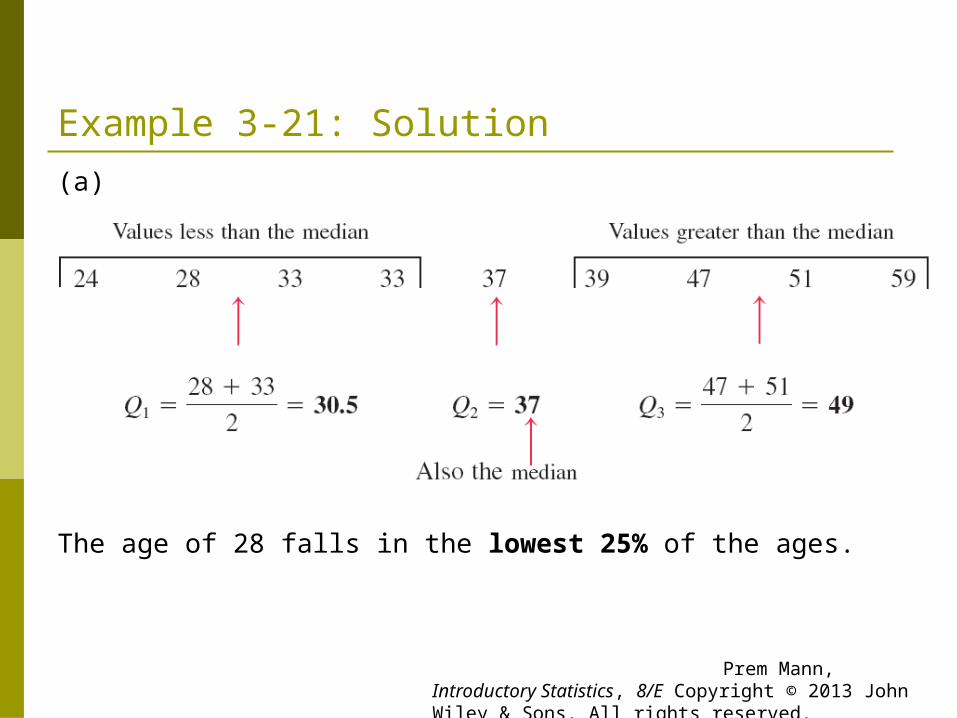
Example 3-21: Solution
(a)
The age of 28 falls in the lowest 25% of the ages.
Prem Mann, Introductory Statistics, 8/E Copyright © 2013 John Wiley & Sons. All rights reserved.
Example 3-21: Solution
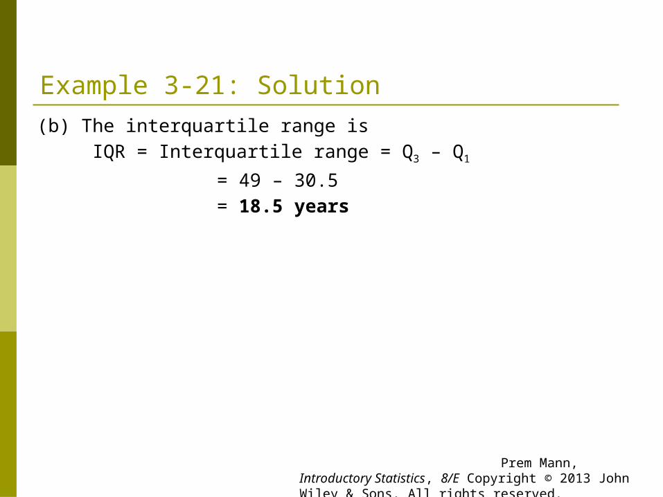
(b) The interquartile range is IQR = Interquartile range = Q3 – Q1
= 49 – 30.5 = 18.5 years
Prem Mann, Introductory Statistics, 8/E Copyright © 2013 John Wiley & Sons. All rights reserved.

Percentiles and Percentile Rank
Prem Mann, Introductory Statistics, 8/E Copyright © 2013 John Wiley & Sons. All rights reserved.

Percentiles and Percentile Rank Calculating Percentiles The (approximate) value of the k th percentile, denoted by Pk,
is
where k denotes the number of the percentile and n represents the sample size.
set data ranked ain th term100
theof Value
knPk
Prem Mann, Introductory Statistics, 8/E Copyright © 2013 John Wiley & Sons. All rights reserved.
Example 3-22 Refer to the data on total compensations (in millions of
dollars) for the year 2010 of the 12 highest-paid CEOs of U.S. companies given in Example 3-20. Find the value of the 60th percentile. Give a brief interpretation of the 60th percentile.
Prem Mann, Introductory Statistics, 8/E Copyright © 2013 John Wiley & Sons. All rights reserved.

Example 3-22: Solution The data arranged in increasing order is as follows:
21.6 21.7 22.9 25.2 26.5 28.0 28.2 32.6 32.9 70.1 76.1 84.5
The position of the 60th percentile is
term 7th term th 20.7100
)12)(60(
100
kn
Prem Mann, Introductory Statistics, 8/E Copyright © 2013 John Wiley & Sons. All rights reserved.
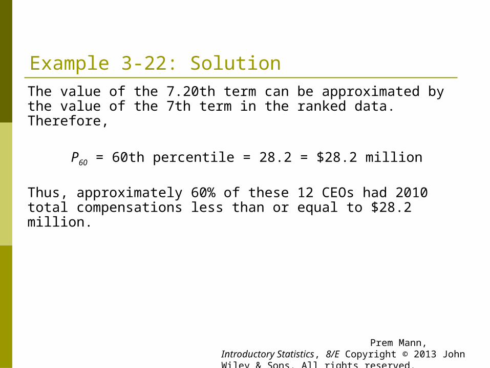
Example 3-22: Solution The value of the 7.20th term can be approximated by the value
of the 7th term in the ranked data. Therefore,
P60 = 60th percentile = 28.2 = $28.2 million
Thus, approximately 60% of these 12 CEOs had 2010 total compensations less than or equal to $28.2 million.
Prem Mann, Introductory Statistics, 8/E Copyright © 2013 John Wiley & Sons. All rights reserved.

Percentiles and Percentile Rank
Finding Percentile Rank of a Value
100set data the in valuesof number Total
than less valuesof Number
of rank Percentile
i
i
x
x
Prem Mann, Introductory Statistics, 8/E Copyright © 2013 John Wiley & Sons. All rights reserved.
Example 3-23 Refer to the data on total compensations (in millions of
dollars) for the year 2010 of the 12 highest-paid CEOs of U.S. companies given in Example 3-20. Find the percentile rank for $26.5 million (2010 total compensation of Alan Mulally, CEO of Ford Motor). Give a brief interpretation of this percentile rank.
Prem Mann, Introductory Statistics, 8/E Copyright © 2013 John Wiley & Sons. All rights reserved.

Example 3-23: Solution The data on revenues arranged in increasing order is as
follows:
21.6 21.7 22.9 25.2 26.5 28.0 28.2 32.6 32.9 70.1 76.1 84.5
In this data set, 4 of the 12 values are less than $26.5 million. Hence,
Percentile rank of 26.5=4
12×100=33.33%
Prem Mann, Introductory Statistics, 8/E Copyright © 2013 John Wiley & Sons. All rights reserved.
Example 3-23: Solution Rounding this answer to the nearest integral value, we can
state that about 33% of these 12 CEOs had 2010 total compensations of less than $26.5 million. Hence, 67% of these 12 CEOs had $26.5 million or higher total compensations in 2010.
Prem Mann, Introductory Statistics, 8/E Copyright © 2013 John Wiley & Sons. All rights reserved.

BOX-AND-WHISKER PLOT Definition A plot that shows the center, spread, and skewness of a data
set. It is constructed by drawing a box and two whiskers that use the median, the first quartile, the third quartile, and the smallest and the largest values in the data set between the lower and the upper inner fences.
Prem Mann, Introductory Statistics, 8/E Copyright © 2013 John Wiley & Sons. All rights reserved.

Example 3-24 The following data are the incomes (in thousands of dollars)
for a sample of 12 households.
75 69 84 112 74 104 81 90 94 144 79 98
Construct a box-and-whisker plot for these data.
Prem Mann, Introductory Statistics, 8/E Copyright © 2013 John Wiley & Sons. All rights reserved.

Example 3-24: Solution Step 1. First, rank the data in increasing order and calculate
the values of the median, the first quartile, the third quartile, and the interquartile range. The ranked data are
69 74 75 79 81 84 90 94 98 104 112 144
Median = (84 + 90) / 2 = 87 Q1 = (75 + 79) / 2 = 77 Q3 = (98 + 104) / 2 = 101 IQR = Q3 – Q1 = 101 – 77 = 24
Prem Mann, Introductory Statistics, 8/E Copyright © 2013 John Wiley & Sons. All rights reserved.

Example 3-24: Solution Step 2. Find the points that are 1.5 x IQR below Q1 and 1.5 x
IQR above Q3.
1.5 x IQR = 1.5 x 24 = 36 Lower inner fence = Q1 – 36 = 77 – 36 = 41 Upper inner fence = Q3 + 36 = 101 + 36 = 137
Prem Mann, Introductory Statistics, 8/E Copyright © 2013 John Wiley & Sons. All rights reserved.

Example 3-24: Solution Step 3. Determine the smallest and the largest values in the
given data set within the two inner fences.
Smallest value within the two inner fences = 69 Largest value within the two inner fences = 112
Prem Mann, Introductory Statistics, 8/E Copyright © 2013 John Wiley & Sons. All rights reserved.

Example 3-24: Solution Step 4. Draw a horizontal line and mark the income levels
on it such that all the values in the given data set are covered. The result of this step is shown in Figure 3.13.
Prem Mann, Introductory Statistics, 8/E Copyright © 2013 John Wiley & Sons. All rights reserved.
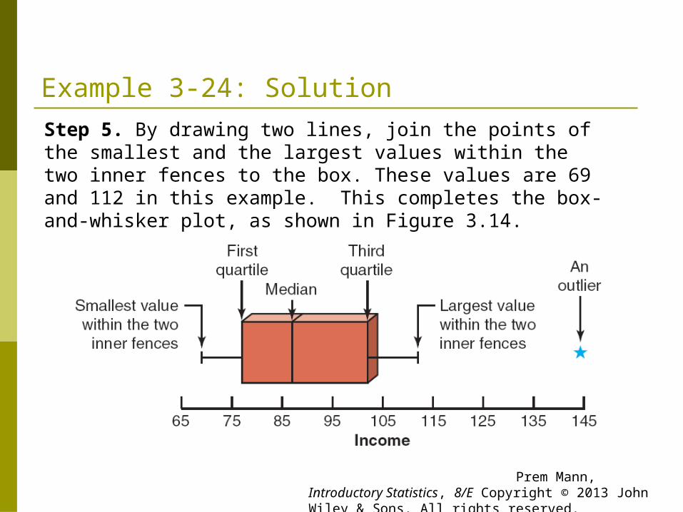
Example 3-24: Solution Step 5. By drawing two lines, join the points of the
smallest and the largest values within the two inner fences to the box. These values are 69 and 112 in this example. This completes the box-and-whisker plot, as shown in Figure 3.14.
Prem Mann, Introductory Statistics, 8/E Copyright © 2013 John Wiley & Sons. All rights reserved.
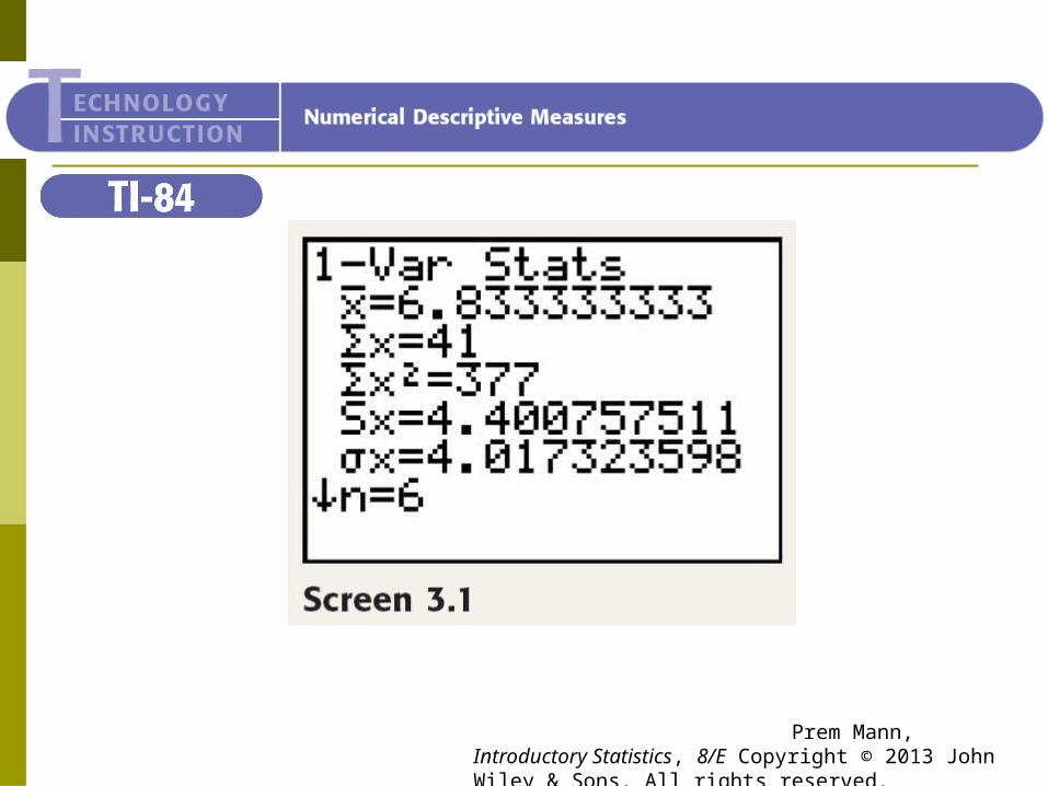
TI-84
Prem Mann, Introductory Statistics, 8/E Copyright © 2013 John Wiley & Sons. All rights reserved.

TI-84
Prem Mann, Introductory Statistics, 8/E Copyright © 2013 John Wiley & Sons. All rights reserved.

TI-84
Prem Mann, Introductory Statistics, 8/E Copyright © 2013 John Wiley & Sons. All rights reserved.
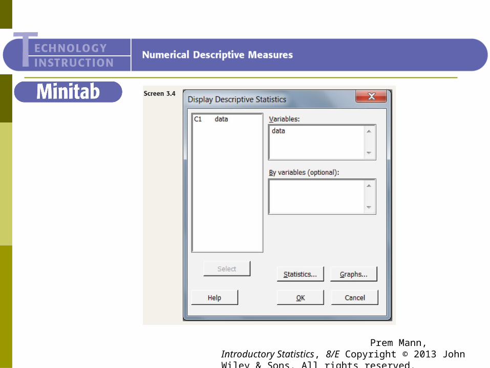
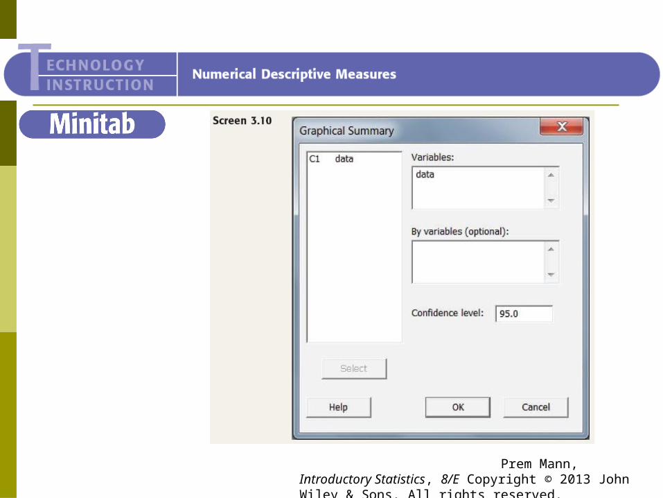
Minitab
Prem Mann, Introductory Statistics, 8/E Copyright © 2013 John Wiley & Sons. All rights reserved.

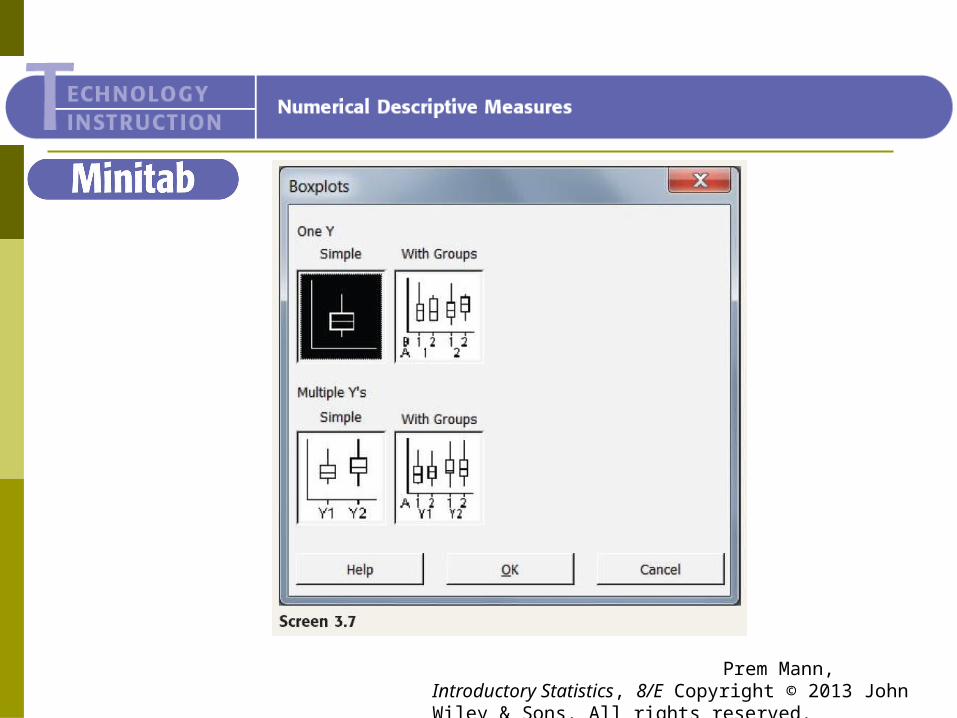
Minitab
Prem Mann, Introductory Statistics, 8/E Copyright © 2013 John Wiley & Sons. All rights reserved.

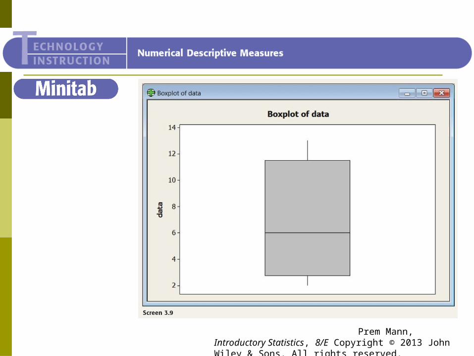
Minitab
Prem Mann, Introductory Statistics, 8/E Copyright © 2013 John Wiley & Sons. All rights reserved.
Minitab
Prem Mann, Introductory Statistics, 8/E Copyright © 2013 John Wiley & Sons. All rights reserved.

Minitab
Prem Mann, Introductory Statistics, 8/E Copyright © 2013 John Wiley & Sons. All rights reserved.
Minitab
Prem Mann, Introductory Statistics, 8/E Copyright © 2013 John Wiley & Sons. All rights reserved.
Minitab
Prem Mann, Introductory Statistics, 8/E Copyright © 2013 John Wiley & Sons. All rights reserved.

Minitab
Prem Mann, Introductory Statistics, 8/E Copyright © 2013 John Wiley & Sons. All rights reserved.

Excel
Prem Mann, Introductory Statistics, 8/E Copyright © 2013 John Wiley & Sons. All rights reserved.

Excel
Prem Mann, Introductory Statistics, 8/E Copyright © 2013 John Wiley & Sons. All rights reserved.

Excel
Prem Mann, Introductory Statistics, 8/E Copyright © 2013 John Wiley & Sons. All rights reserved.


