1 Chapter 3 Present Value and Securities Valuation The objectives of this chapter are to enable you to: ! Value cash flows to be paid in the future ! Value series of cash flows, including annuities and perpetuities ! Value growing annuities and perpetuities ! Value cash flows associated with stocks and bonds ! Understand how to amortize a loan 3.A. INTRODUCTION Cash flows realized at the present time have a greater value to investors than cash flows realized later for the following reasons: 1. Inflation: The purchasing power of money tends to decline over time. 2. Risk: One never knows with certainty whether he will actually realize the cash flow that he is expecting. 3. The option to either spend money now or defer spending it is likely to be worth more than being forced to defer spending the money. The purpose of the Present Value concept is to provide a means of expressing the value of a future cash flow in terms of current cash flows. That is, the Present Value concept is used to determine how much an investor would pay now for the promise of some cash flow to be received at a later date. The present value of this cash flow would be a function of inflation, the length of wait before the cash flow is received, its riskiness and the time value an investor associates with money (how much he needs money now as opposed to later). Perhaps the easiest way to account for these factors when evaluating a future cash flow is to discount it in the following manner: (3.1) n n k CF PV ) 1 ( where (CF n ) is the cash flow to be received in year (n), (k) is an appropriate discount rate accounting for risk, inflation, and the investor's time value associated with money, and PV is the present value of that cash flow. The discount rate enables us to evaluate a future cash flow in terms of cash flows realized today. Thus, the maximum a rational investor would be willing to pay for an investment yielding a $9000 cash flow in six years assuming a discount rate of 15% would be $3891, determined as follows:
Transcript
1
Chapter 3 Present Value and Securities Valuation
The objectives of this chapter are to enable you to: ! Value cash flows to be paid in the future
! Value series of cash flows, including annuities and perpetuities
! Value growing annuities and perpetuities
! Value cash flows associated with stocks and bonds
! Understand how to amortize a loan
3.A. INTRODUCTION Cash flows realized at the present time have a greater value to investors than cash flows
realized later for the following reasons:
1. Inflation: The purchasing power of money tends to decline over time.
2. Risk: One never knows with certainty whether he will actually realize the cash flow
that he is expecting.
3. The option to either spend money now or defer spending it is likely to be worth
more than being forced to defer spending the money.
The purpose of the Present Value concept is to provide a means of expressing the value of a future
cash flow in terms of current cash flows. That is, the Present Value concept is used to determine
how much an investor would pay now for the promise of some cash flow to be received at a later
date. The present value of this cash flow would be a function of inflation, the length of wait before
the cash flow is received, its riskiness and the time value an investor associates with money (how
much he needs money now as opposed to later). Perhaps the easiest way to account for these
factors when evaluating a future cash flow is to discount it in the following manner:
(3.1) n
n
k
CFPV
)1(
where (CFn) is the cash flow to be received in year (n), (k) is an appropriate discount rate
accounting for risk, inflation, and the investor's time value associated with money, and PV is the
present value of that cash flow. The discount rate enables us to evaluate a future cash flow in terms
of cash flows realized today. Thus, the maximum a rational investor would be willing to pay for an
investment yielding a $9000 cash flow in six years assuming a discount rate of 15% would be
$3891, determined as follows:
Chapter 3
2
95.3890$31306.2
9000$
)151(
9000$6
PV
In the above example, we simply assumed a fifteen percent discount rate. Realistically,
perhaps the easiest value to substitute for (k) is the current interest or return rate on loans or other
investments of similar duration and riskiness. However, this market determined interest rate may
not consider the individual investor's time preferences for money. Furthermore, the investor may
find difficulty in locating a loan (or other investment) of similar duration and riskiness. For these
reasons, more scientific methods for determining appropriate discount rates will be discussed later.
In any case, the discount rate should account for inflation, the riskiness of the investment and the
investor's time value for money.
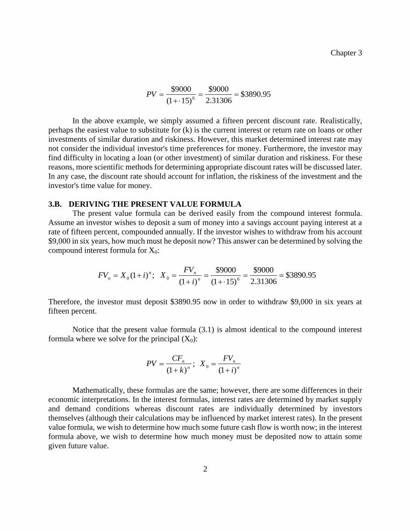
3.B. DERIVING THE PRESENT VALUE FORMULA The present value formula can be derived easily from the compound interest formula.
Assume an investor wishes to deposit a sum of money into a savings account paying interest at a
rate of fifteen percent, compounded annually. If the investor wishes to withdraw from his account
$9,000 in six years, how much must he deposit now? This answer can be determined by solving the
compound interest formula for X0:
;)1(0
n
n iXFV 95.3890$31306.2
9000$
)151(
9000$
)1( 60
n
n
i
FVX
Therefore, the investor must deposit $3890.95 now in order to withdraw $9,000 in six years at
fifteen percent.
Notice that the present value formula (3.1) is almost identical to the compound interest
formula where we solve for the principal (X0):
n
n
k
CFPV
)1( ;
n
n
i
FVX
)1(0
Mathematically, these formulas are the same; however, there are some differences in their
economic interpretations. In the interest formulas, interest rates are determined by market supply
and demand conditions whereas discount rates are individually determined by investors
themselves (although their calculations may be influenced by market interest rates). In the present
value formula, we wish to determine how much some future cash flow is worth now; in the interest
formula above, we wish to determine how much money must be deposited now to attain some
given future value.
Present Value and Securities Valuation
3
3.C. PRESENT VALUE OF A SERIES OF CASH FLOWS
If an investor wishes to evaluate a series of cash flows, he needs only to discount each
separately and then sum the present values of each of the cash flows. Thus, the present value of a
series of cash flows (CFt) received in time period (t) can be determined by the following
expression:1
(3.2) t
tn
t k
CFPV
)1(1
For example, if an investment were expected to yield annual cash flows of $200 for each of the
next five years, assuming a discount rate of 5%, its present value would be $865.90:
1)05.1(
200
PV
2)05.1(
200
3)05.1(
200
4)05.1(
200
5)05.1(
200
=865.90
Therefore, the maximum price an individual should pay for this investment is $865.90 even though
the cash flows yielded by the investment total $1000. Because the individual must wait up to five
years before receiving the $1000, the investment is worth only $865.90. Use of the present value
series formula does not require that cash flows (CFt) in each year be identical, as does the annuity
model presented in the next section.
3.D. ANNUITY MODELS The expression for determining the present value of a series of cash flows can be quite
cumbersome, particularly when the payments extend over a long period of time. This formula
requires that (n) cash flows be discounted separately and then summed. When (n) is large, this task
may be rather time-consuming. If the annual cash flows are identical and are to be discounted at
the same rate, an annuity formula can be a useful time-saving device. The same problem discussed
in the previous section can be solved using the following annuity formula:
(3.3)
nAkk
CFPV
)1(
11
1Readers who are uncomfortable with the summation notation may wish to consult the
mathematics appendix at the end of the text.
Chapter 3
4
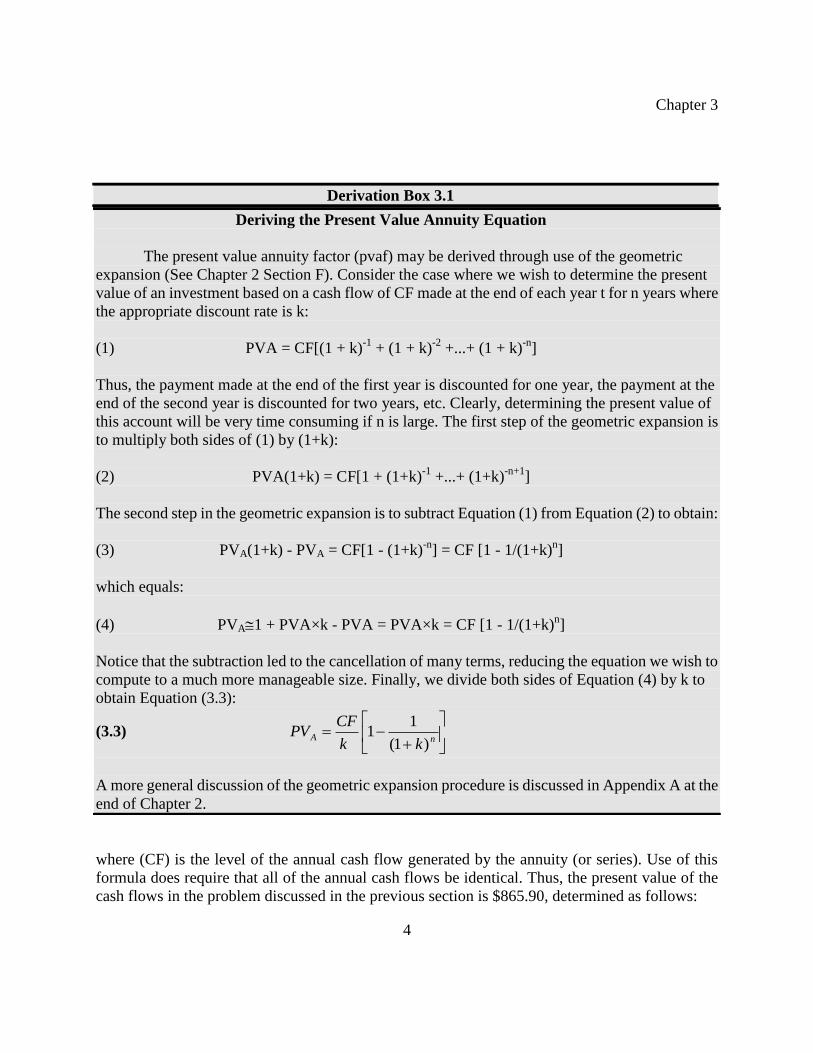
where (CF) is the level of the annual cash flow generated by the annuity (or series). Use of this
formula does require that all of the annual cash flows be identical. Thus, the present value of the
cash flows in the problem discussed in the previous section is $865.90, determined as follows:
Deriving the Present Value Annuity Equation
The present value annuity factor (pvaf) may be derived through use of the geometric
expansion (See Chapter 2 Section F). Consider the case where we wish to determine the present
value of an investment based on a cash flow of CF made at the end of each year t for n years where
the appropriate discount rate is k:
(1) PVA = CF[(1 + k)-1
+ (1 + k)-2
+...+ (1 + k)-n
]
Thus, the payment made at the end of the first year is discounted for one year, the payment at the
end of the second year is discounted for two years, etc. Clearly, determining the present value of
this account will be very time consuming if n is large. The first step of the geometric expansion is
to multiply both sides of (1) by (1+k):
(2) PVA(1+k) = CF[1 + (1+k)-1
+...+ (1+k)-n+1
]
The second step in the geometric expansion is to subtract Equation (1) from Equation (2) to obtain:
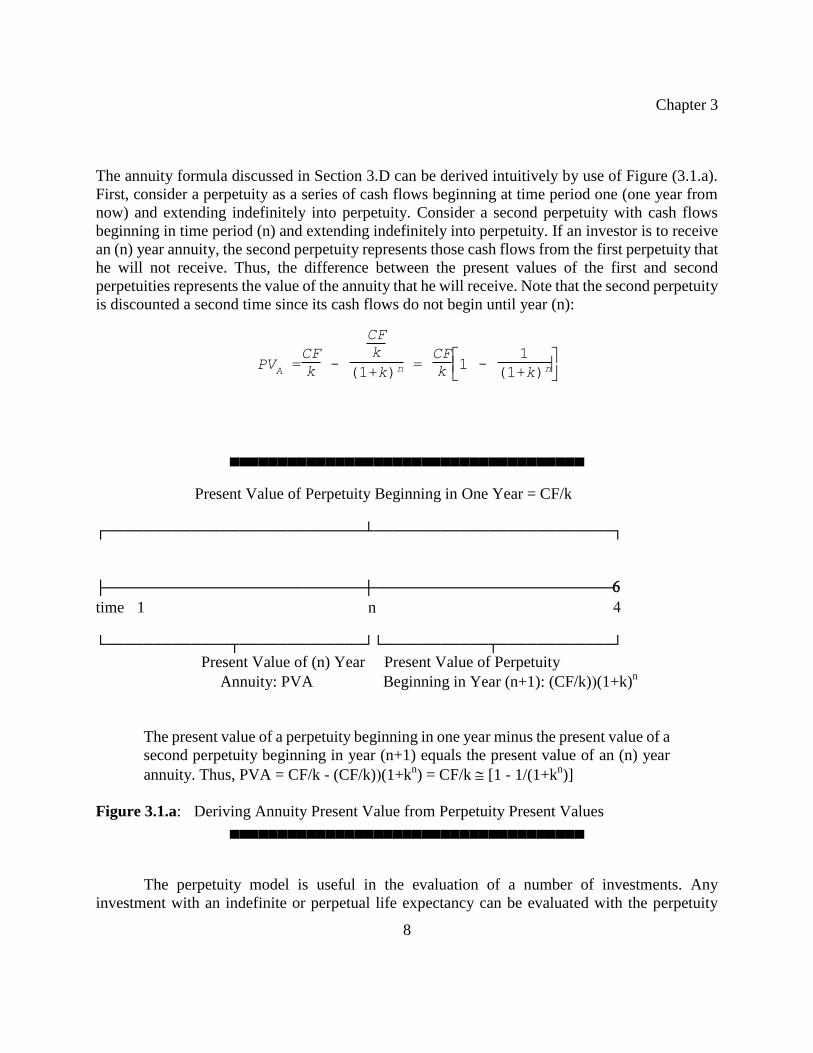
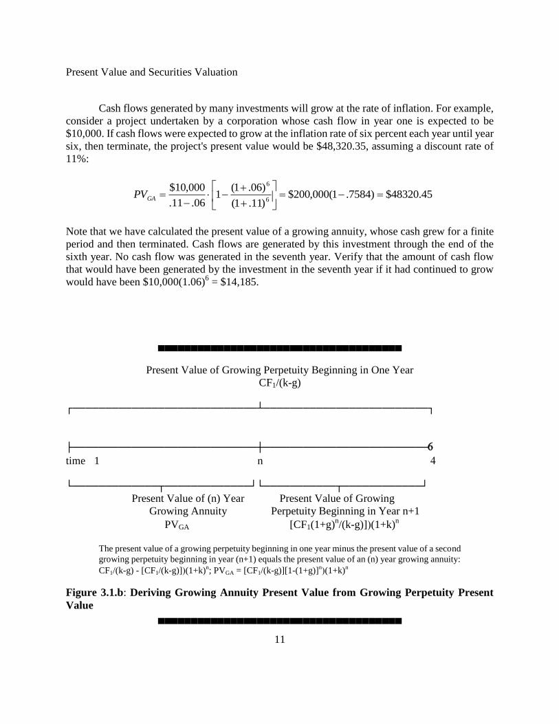
Figure 3.1.b: Deriving Growing Annuity Present Value from Growing Perpetuity Present
Value ▄▄▄▄▄▄▄▄▄▄▄▄▄▄▄▄▄▄▄▄▄▄▄▄▄▄▄▄▄▄▄▄▄▄▄▄▄
Chapter 3
12
3.H. STOCK VALUATION Consider a stock whose annual dividend next year is projected to be $50. This payment is
expected to grow at an annual rate of 5% in subsequent years. An investor has determined that the
appropriate discount rate for this stock is 10%. The current value of this stock is $1000, determined
by the growing perpetuity model:
1000$05.10.
50$
gpPV
This model is often referred to as the Gordon Stock Pricing Model. It may seem that this
model assumes that the stock will be held by the investor forever. But what if the investor intends
to sell the stock in five years? Its value would be determined by the sum of the present values of
cash flows the investor does expect to receive:
n
n
GAk
g
gk
DIVPV
)1(
)1(11
where (Pn) is the price the investor expects to receive when he sells the stock in year (n); and
(DIV1) is the dividend payment the investor expects to receive in year one. The present value of the
dividends the investor expects to receive is $207.53:
53.207)10.1(
)05.1(1
05.10.
50$5
5
GAPV
The selling price of the stock in year five will be a function of the dividend payments the
prospective purchaser expects to receive beginning in year six. Thus, in year five, the prospective
purchaser will pay $1,276.28 for the stock, based on his initial dividend payment of $63.81,
determined by the following equations:
DIV6 = DIV1 (1+.05)6-1
= $63.81
Stock value in year five = 63.81/(.10-.05) = $1276.28
The present value of the $1,276.28 the investor will receive when he sells the stock at the end of
the fifth year is $792.47:
57.792$)1.1(
28.1276$5
PV
Present Value and Securities Valuation
13
The total stock value will be the sum of the present values of the dividends received by the investor
and his cash flows received from the sale of the stock. Thus, the current value of the stock is
$207.53 plus $792.47, or $1000. This is exactly the same sum determined by the growing
perpetuity model earlier; therefore, the growing perpetuity model can be used to evaluate a stock
even when the investor expects to sell it.
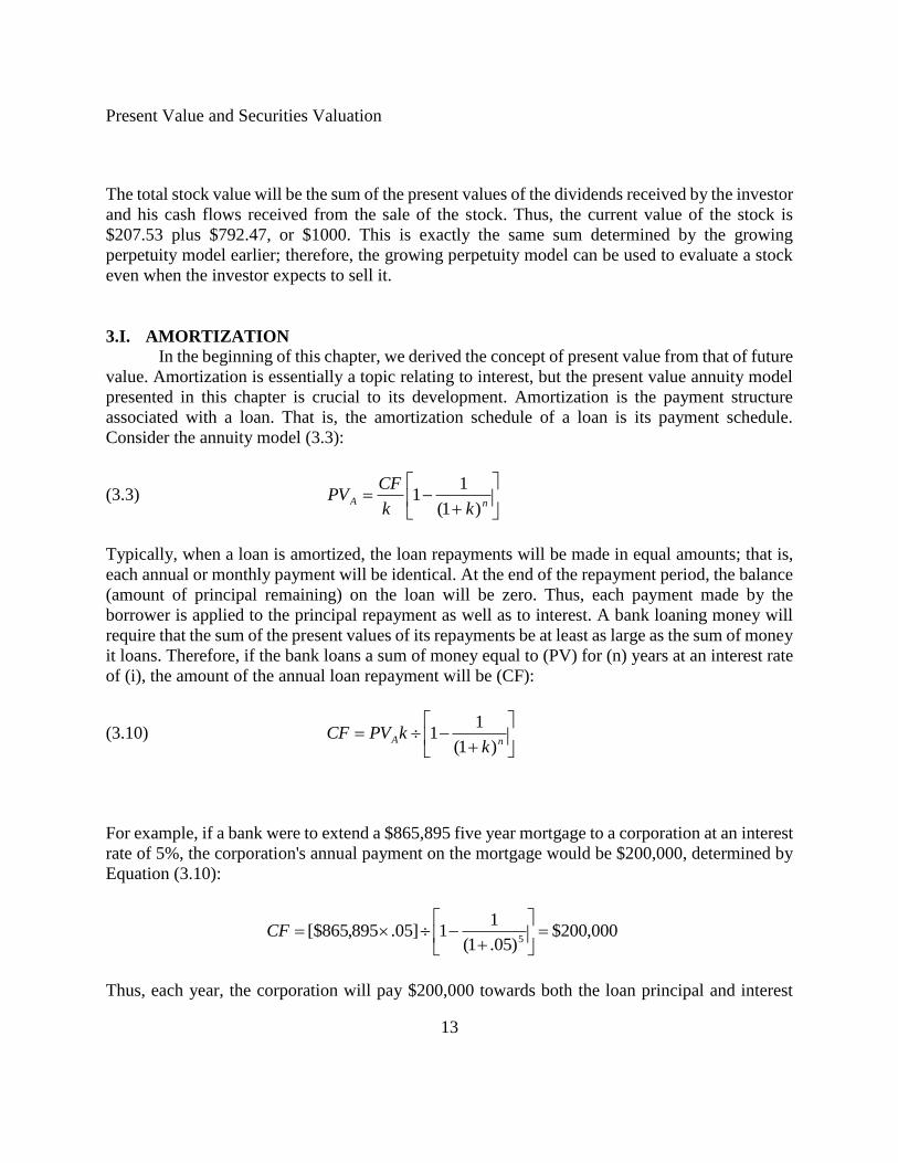
3.I. AMORTIZATION
In the beginning of this chapter, we derived the concept of present value from that of future
value. Amortization is essentially a topic relating to interest, but the present value annuity model
presented in this chapter is crucial to its development. Amortization is the payment structure
associated with a loan. That is, the amortization schedule of a loan is its payment schedule.
Consider the annuity model (3.3):
(3.3)
nAkk
CFPV
)1(
11
Typically, when a loan is amortized, the loan repayments will be made in equal amounts; that is,
each annual or monthly payment will be identical. At the end of the repayment period, the balance
(amount of principal remaining) on the loan will be zero. Thus, each payment made by the
borrower is applied to the principal repayment as well as to interest. A bank loaning money will
require that the sum of the present values of its repayments be at least as large as the sum of money
it loans. Therefore, if the bank loans a sum of money equal to (PV) for (n) years at an interest rate
of (i), the amount of the annual loan repayment will be (CF):
(3.10)
nAk
kPVCF)1(
11
For example, if a bank were to extend a $865,895 five year mortgage to a corporation at an interest
rate of 5%, the corporation's annual payment on the mortgage would be $200,000, determined by
Equation (3.10):
000,200$)05.1(
11]05.895,865[$
5
CF
Thus, each year, the corporation will pay $200,000 towards both the loan principal and interest
Chapter 3
14
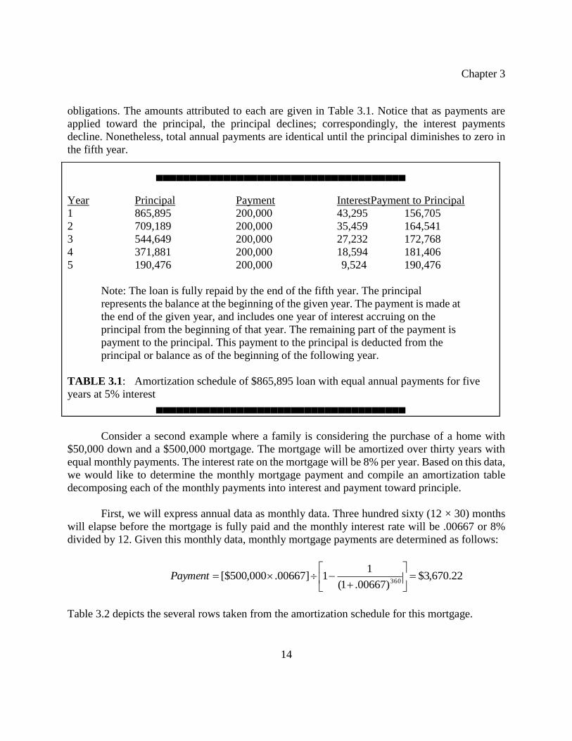
obligations. The amounts attributed to each are given in Table 3.1. Notice that as payments are
applied toward the principal, the principal declines; correspondingly, the interest payments
decline. Nonetheless, total annual payments are identical until the principal diminishes to zero in
the fifth year.
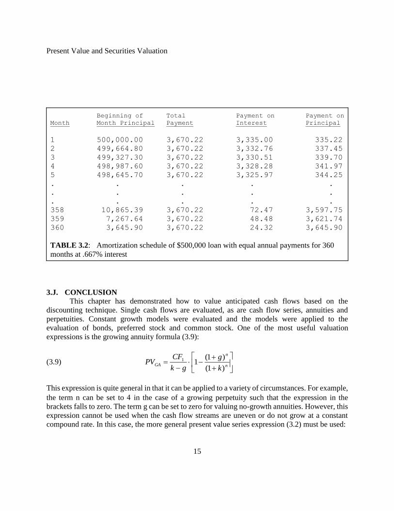
Consider a second example where a family is considering the purchase of a home with
$50,000 down and a $500,000 mortgage. The mortgage will be amortized over thirty years with
equal monthly payments. The interest rate on the mortgage will be 8% per year. Based on this data,
we would like to determine the monthly mortgage payment and compile an amortization table
decomposing each of the monthly payments into interest and payment toward principle.
First, we will express annual data as monthly data. Three hundred sixty (12 × 30) months
will elapse before the mortgage is fully paid and the monthly interest rate will be .00667 or 8%
divided by 12. Given this monthly data, monthly mortgage payments are determined as follows:
22.670,3$)00667.1(
11]00667.000,500[$
360
Payment
Table 3.2 depicts the several rows taken from the amortization schedule for this mortgage.
▄▄▄▄▄▄▄▄▄▄▄▄▄▄▄▄▄▄▄▄▄▄▄▄▄▄▄▄▄▄▄▄▄▄▄▄▄
Year Principal Payment InterestPayment to Principal
1 865,895 200,000 43,295 156,705
2 709,189 200,000 35,459 164,541
3 544,649 200,000 27,232 172,768
4 371,881 200,000 18,594 181,406
5 190,476 200,000 9,524 190,476
Note: The loan is fully repaid by the end of the fifth year. The principal
represents the balance at the beginning of the given year. The payment is made at
the end of the given year, and includes one year of interest accruing on the
principal from the beginning of that year. The remaining part of the payment is
payment to the principal. This payment to the principal is deducted from the
principal or balance as of the beginning of the following year.
TABLE 3.1: Amortization schedule of $865,895 loan with equal annual payments for five
years at 5% interest ▄▄▄▄▄▄▄▄▄▄▄▄▄▄▄▄▄▄▄▄▄▄▄▄▄▄▄▄▄▄▄▄▄▄▄▄▄
Present Value and Securities Valuation
15
Beginning of Total Payment on Payment on
Month Month Principal Payment Interest Principal
1 500,000.00 3,670.22 3,335.00 335.22
2 499,664.80 3,670.22 3,332.76 337.45
3 499,327.30 3,670.22 3,330.51 339.70
4 498,987.60 3,670.22 3,328.28 341.97
5 498,645.70 3,670.22 3,325.97 344.25
. . . . .
. . . . .
. . . . .
358 10,865.39 3,670.22 72.47 3,597.75
359 7,267.64 3,670.22 48.48 3,621.74
360 3,645.90 3,670.22 24.32 3,645.90
TABLE 3.2: Amortization schedule of $500,000 loan with equal annual payments for 360
months at .667% interest
3.J. CONCLUSION
This chapter has demonstrated how to value anticipated cash flows based on the
discounting technique. Single cash flows are evaluated, as are cash flow series, annuities and
perpetuities. Constant growth models were evaluated and the models were applied to the
evaluation of bonds, preferred stock and common stock. One of the most useful valuation
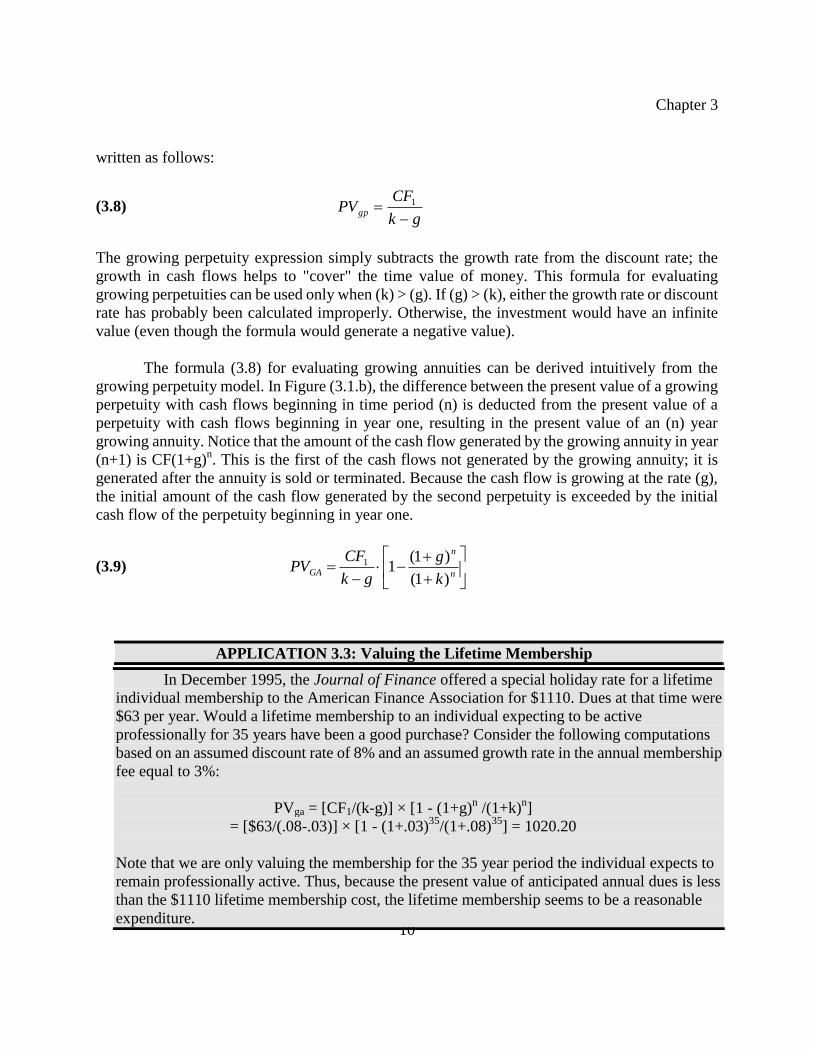
expressions is the growing annuity formula (3.9):
(3.9)
n
n
GAk
g
gk
CFPV
)1(
)1(11
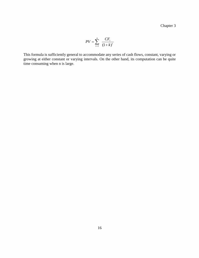
This expression is quite general in that it can be applied to a variety of circumstances. For example,
the term n can be set to in the case of a growing perpetuity such that the expression in the
brackets falls to zero. The term g can be set to zero for valuing no-growth annuities. However, this
expression cannot be used when the cash flow streams are uneven or do not grow at a constant
compound rate. In this case, the more general present value series expression (3.2) must be used:
Chapter 3
16
t
tn
t k
CFPV
)1(1
This formula is sufficiently general to accommodate any series of cash flows, constant, varying or
growing at either constant or varying intervals. On the other hand, its computation can be quite
time consuming when n is large.
Present Value and Securities Valuation
17
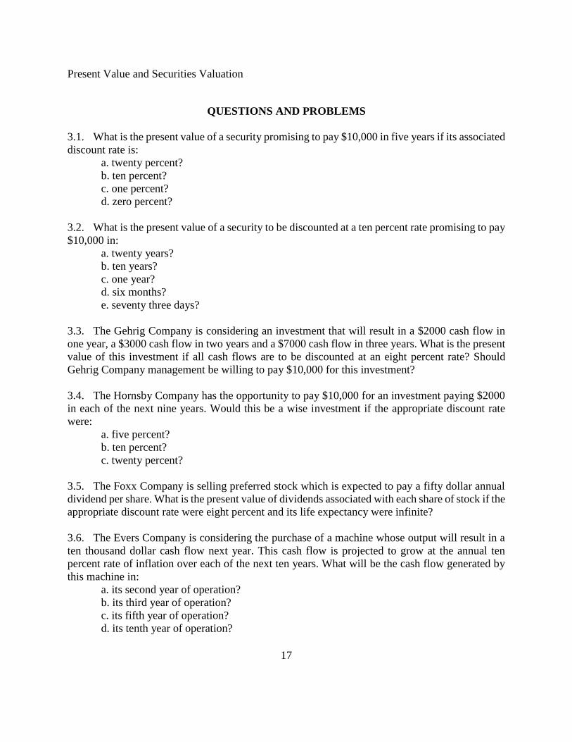
QUESTIONS AND PROBLEMS
3.1. What is the present value of a security promising to pay $10,000 in five years if its associated
discount rate is:
a. twenty percent?
b. ten percent?
c. one percent?
d. zero percent?
3.2. What is the present value of a security to be discounted at a ten percent rate promising to pay
$10,000 in:
a. twenty years?
b. ten years?
c. one year?
d. six months?
e. seventy three days?
3.3. The Gehrig Company is considering an investment that will result in a $2000 cash flow in
one year, a $3000 cash flow in two years and a $7000 cash flow in three years. What is the present
value of this investment if all cash flows are to be discounted at an eight percent rate? Should
Gehrig Company management be willing to pay $10,000 for this investment?
3.4. The Hornsby Company has the opportunity to pay $10,000 for an investment paying $2000
in each of the next nine years. Would this be a wise investment if the appropriate discount rate
were:
a. five percent?
b. ten percent?
c. twenty percent?
3.5. The Foxx Company is selling preferred stock which is expected to pay a fifty dollar annual
dividend per share. What is the present value of dividends associated with each share of stock if the
appropriate discount rate were eight percent and its life expectancy were infinite?
3.6. The Evers Company is considering the purchase of a machine whose output will result in a
ten thousand dollar cash flow next year. This cash flow is projected to grow at the annual ten
percent rate of inflation over each of the next ten years. What will be the cash flow generated by
this machine in:
a. its second year of operation?
b. its third year of operation?
c. its fifth year of operation?
d. its tenth year of operation?
Chapter 3
18
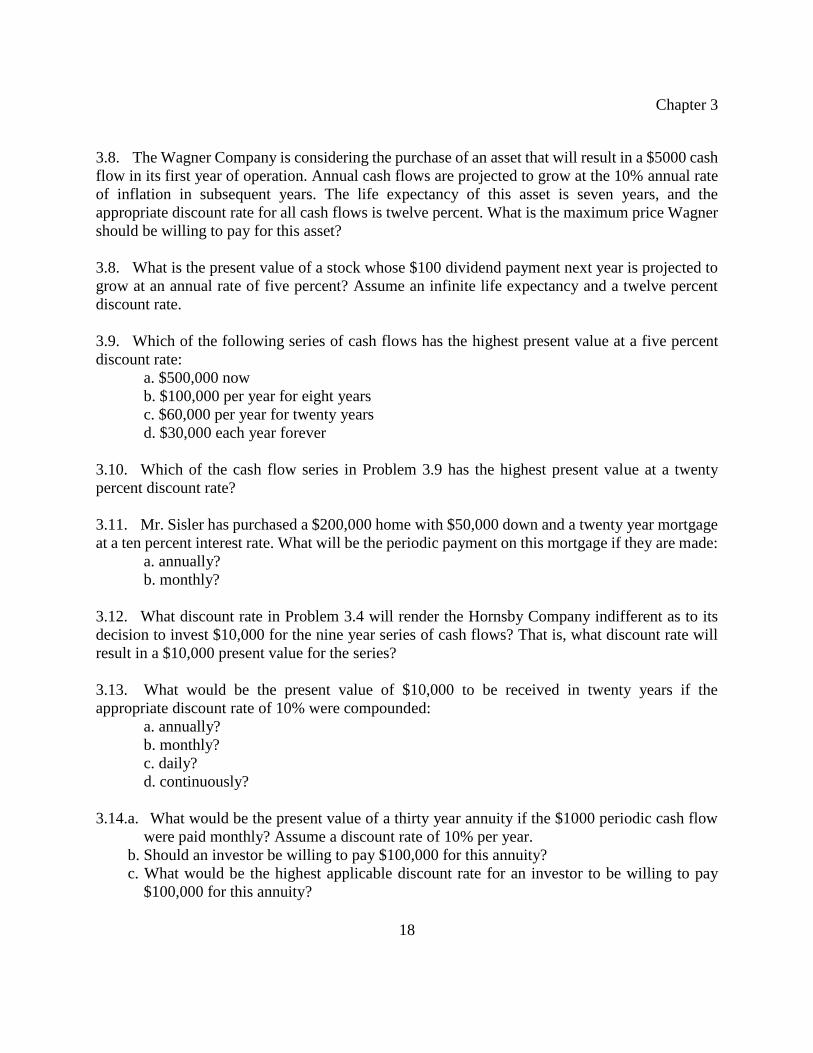
3.8. The Wagner Company is considering the purchase of an asset that will result in a $5000 cash
flow in its first year of operation. Annual cash flows are projected to grow at the 10% annual rate
of inflation in subsequent years. The life expectancy of this asset is seven years, and the
appropriate discount rate for all cash flows is twelve percent. What is the maximum price Wagner
should be willing to pay for this asset?
3.8. What is the present value of a stock whose $100 dividend payment next year is projected to
grow at an annual rate of five percent? Assume an infinite life expectancy and a twelve percent
discount rate.
3.9. Which of the following series of cash flows has the highest present value at a five percent
discount rate:
a. $500,000 now
b. $100,000 per year for eight years
c. $60,000 per year for twenty years
d. $30,000 each year forever
3.10. Which of the cash flow series in Problem 3.9 has the highest present value at a twenty
percent discount rate?
3.11. Mr. Sisler has purchased a $200,000 home with $50,000 down and a twenty year mortgage
at a ten percent interest rate. What will be the periodic payment on this mortgage if they are made:
a. annually?
b. monthly?
3.12. What discount rate in Problem 3.4 will render the Hornsby Company indifferent as to its
decision to invest $10,000 for the nine year series of cash flows? That is, what discount rate will
result in a $10,000 present value for the series?
3.13. What would be the present value of $10,000 to be received in twenty years if the
appropriate discount rate of 10% were compounded:
a. annually?
b. monthly?
c. daily?
d. continuously?
3.14.a. What would be the present value of a thirty year annuity if the $1000 periodic cash flow
were paid monthly? Assume a discount rate of 10% per year.
b. Should an investor be willing to pay $100,000 for this annuity?
c. What would be the highest applicable discount rate for an investor to be willing to pay
$100,000 for this annuity?
Present Value and Securities Valuation
19
3.15. Demonstrate how to derive an expression to determine the present value of a growing
annuity. Use the geometric expansion to derive Equation (3.12) in the text.
3.16. An individual has purchased a home with $30,000 down and a $300,000 mortgage. The
mortgage will be amortized over thirty years with equal monthly payments. The interest rate on the
mortgage will be 9% per year. Based on this data, answer the following:
a. How many months will elapse before the mortgage is fully paid?
b. What is the monthly interest rate on the mortgage?
c. What will be the monthly mortgage payment?
d. Set up an amortization table to illustrate interest payments, payments on the principal and
mortgage balances (beginning of month principal).
3.17. Suppose an investor has the opportunity to invest in a stock currently selling for $100 per
share. The stock is expected to pay a $5 dividend next year (at the end of year 1). In each
subsequent year until the third year, the annual dividend is expected to grow at a rate of 15%.
Starting in the fourth year, the annual dividend will grow at an annual rate of 6% until the sixth
year. Starting in the seventh year, dividends will not grow. All cash flows are to be discounted at
an annual rate of 8%. Should the stock be purchased at its current price?
Chapter 3
20
APPENDIX
3.A. TIME VALUE SPREADSHEET APPLICATIONS
Spreadsheets are very useful for time value calculations, particularly when there are either
a large number of time periods or a large number of potential outcomes. Not are most time value
formulas easy to enter into cells, but the toolbar the top of the Excel screen should have the Paste
Function button (fx) which will direct the user to a variety of time value functions. By left-clicking
the Paste Function (fx), the user will be directed to the Paste Function menu. From the Paste
Function menu, one can select the Financial sub-menu. In the Financial sub-menu, scroll down to
select the appropriate time value function. Pay close attention to the proper format and arguments
for entry. Table 3.B.1 below lists a number of time value functions which may be accessed through
the Paste Function menu along with the example and notes.
While the formulas entered into Table 3.B.1 make use of specialized Paste Functions for
Finance, the spreadsheet user can enter his own simple formulas. For example, suppose that the
user enters a cash flow in cell A1, a discount rate in cell A2 and a payment or termination period
into cell A3. The present value of this cash flow can be found with =A1/(1+A2)^A3 or, in the case
of an annuity, with =A1*((1/A2)-(1/(A2*(1+A2)^A3))). Now, enter a deposit amount into cell A1,
an interest rate in cell A2 and a payment date or termination date in cell A3. Future values can be
found with =A1*(1+A2)^n and =A1*((1/A2)-(1/(A2*(1+A2)^A3)))*(1+A2)^n. These formulas
can easily be adjusted for growth, in which a value for cell A4 may be inserted for the growth rate.
Present Value and Securities Valuation
21
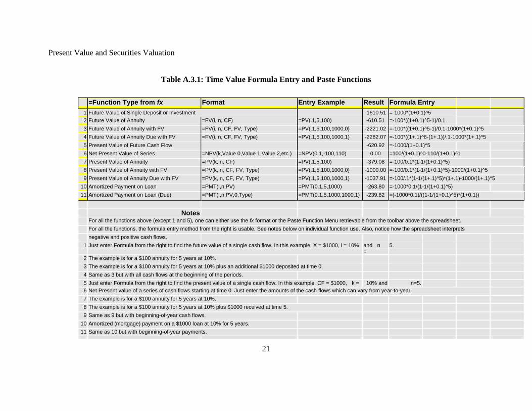
Table A.3.1: Time Value Formula Entry and Paste Functions
=Function Type from fx
Format
Entry Example
Result
Formula Entry
1 Future Value of Single Deposit or Investment
-1610.51
=-1000*(1+0.1)^5
2 Future Value of Annuity =FV(i, n, CF) =PV(.1,5,100) -610.51 =-100*((1+0.1)^5-1)/0.1
3 Future Value of Annuity with FV =FV(i, n, CF, FV, Type) =PV(.1,5,100,1000,0) -2221.02 =-100*((1+0.1)^5-1)/0.1-1000*(1+0.1)^5
4 Future Value of Annuity Due with FV =FV(i, n, CF, FV, Type) =PV(.1,5,100,1000,1) -2282.07 =-100*((1+.1)^6-(1+.1))/.1-1000*(1+.1)^5
5 Present Value of Future Cash Flow -620.92 =-1000/(1+0.1)^5
6 Net Present Value of Series =NPV(k,Value 0,Value 1,Value 2,etc.) =NPV(0.1,-100,110) 0.00 =100/(1+0.1)^0-110/(1+0.1)^1
7 Present Value of Annuity =PV(k, n, CF) =PV(.1,5,100) -379.08 =-100/0.1*(1-1/(1+0.1)^5)
8 Present Value of Annuity with FV =PV(k, n, CF, FV, Type) =PV(.1,5,100,1000,0) -1000.00 =-100/0.1*(1-1/(1+0.1)^5)-1000/(1+0.1)^5
9 Present Value of Annuity Due with FV =PV(k, n, CF, FV, Type) =PV(.1,5,100,1000,1) -1037.91 =-100/.1*(1-1/(1+.1)^5)*(1+.1)-1000/(1+.1)^5
10 Amortized Payment on Loan =PMT(I,n,PV) =PMT(0.1,5,1000) -263.80 =-1000*0.1/(1-1/(1+0.1)^5)
11 Amortized Payment on Loan (Due) =PMT(I,n,PV,0,Type) =PMT(0.1,5,1000,1000,1) -239.82 =(-1000*0.1)/((1-1/(1+0.1)^5)*(1+0.1))
Notes
For all the functions above (except 1 and 5), one can either use the fx format or the Paste Function Menu retrievable from the toolbar above the spreadsheet.
For all the functions, the formula entry method from the right is usable. See notes below on individual function use. Also, notice how the spreadsheet interprets
negative and positive cash flows.
1 Just enter Formula from the right to find the future value of a single cash flow. In this example, X = $1000, i = 10% and n =
5.
2 The example is for a $100 annuity for 5 years at 10%.
3 The example is for a $100 annuity for 5 years at 10% plus an additional $1000 deposited at time 0.
4 Same as 3 but with all cash flows at the beginning of the periods.
5 Just enter Formula from the right to find the present value of a single cash flow. In this example, CF = $1000, k = 10% and n=5. 6 Net Present value of a series of cash flows starting at time 0. Just enter the amounts of the cash flows which can vary from year-to-year.
7 The example is for a $100 annuity for 5 years at 10%.
8 The example is for a $100 annuity for 5 years at 10% plus $1000 received at time 5.
9 Same as 9 but with beginning-of-year cash flows.
10 Amortized (mortgage) payment on a $1000 loan at 10% for 5 years.
11 Same as 10 but with beginning-of-year payments.