Capital Income Taxation and Resource Allocation

by Hans-Werner Sinn

North Holland: Amsterdam, New York, Oxford and Tokio 1987

Chapter 3: Taxes and the Decision Problem of the Firm

Chapter 3

\:

TAXES AND THE DECISION PROBLEM OF THE FIRM

After examining the intertemporal allocation mechanism in the context of household and firm decisions, we can now move on to an analysis of the role of taxation. This chapter gives an overview of alternative tax systems and studies the way in which they enter the decision problem of the firm. Except for decisions about optimal labor supply, the behavioral implications of taxation are not yet treated. Their analysis is postponed until the following Chapters 4 and 5.

3.1. An Overview of Tax Systems

The task of this Section is to define the theoretical tax systems to be analyzed, drawing on systems that exist in the OECD countries or have come under political consideration. Attention will be focussed primarily on alternative systems o~ ,capital income taxation that are characterized by different degrees of integration of personal income taxation and corporate t3:xation and by different depreciation rules. However, in a rudimentary form, other taxes are also included in the analysis.

Without substantial idealizations, the form,llation of an appropriate model framework cannot be achieved. Thus the idea of the representative household and the representative firm will always be employed, and difficulties like, for example, non-proportional taxes1 are neglected. A tax is

1 The assumption of proportional taxes is not as restrictive as it might appear at first glance. At any rate it is not more restrictive than the assumption of linear 'local approximations of tax functions with the aid of which it is even possible to represent certain elements of progressive taxes. Linear taxes differ from proportional taxes only by the additional consideration of absolute terms in the tax functions. These absolute terms can be interpreted as additional lump sum taxes that, by themselves, do not induce substitution effects. If they have any effect at all, it may be to induce income effects which, however, are excluded from this analysis (compare Introduction). This implies that the tax rates used here should normally be compared to maroinaf rather than average tax rates in real tax systems. Only in the context of share

46 Capital Income Taxation and Resource Allocation

always described by a tax rate and a tax base. The tax rate will be indicated by the Greek letter "t" amended' by a suitable subscript. It will turn out that the algebraic formulations in the later analysis often contain expressions of the kind 1- t. These expressions are called tax factors and are denoted by a "e" with the same subscript as the corresponding r.

3.1.1. The Basic Structure of a Simple Tax System

The tax systems of the various countries are complex and differ in many details but they are, nevertheless, closely related. Everywhere there are personal income taxes, corporate income taxes, consumption taxes, and taxes on the stock of capjtal. In a number of countries there are, moreover, capital gains taxes. Except for corporate income taxes, these taxes are similar in the different countries, and corporate income taxes can be reduced to a small number of different ca~egories.

As a typical representative of the consumption taxes we assume a tax like the European value-added tax that traditionally has been· a major source.of government finance in the Latin countries but during the last two decades has come to dominate throughout the whole of Europe. With regard to the problem of intertemporal allocation, it seems that the value-added tax can be used as a fit:st approximation for a number of specific consumption taxes in the different countries. At any rate, for the sake of this analysis .it can be roughly identi-fied with the retail sales tax that, judged by the revenue it generates, is the most important among all North American sales taxes.2 The tax base is the sales, C, that firms make to private households. Set the net price of the consumption good (and hence the net and gross prices of the investment good) equal to unity. Then the flow of revenue generated at a particular point in time by the va]ue-added tax is

(3.1)

where rv > 0 indicates the tax rate. In economic terms, the value-added tax can also be identified in the present context with the expenditure tax that

valuation (see Chapters 6.1 and 10) will the assumption of proportionality really be needed. These remarks should not, however, discourge rurther research on the problem of progressive mar(Jinal tax rates. Any model that produces the so-called "Miller equilibrium .. would have to incorporate this property explicitly. See Chapter 4.3.4 for details.

2 See Musgrave and Musgrave (1973, pp. 323-326) for further details. It goes without saying that the similarity of the two taxes is limited and that there are problems for which a careful distinction would be necessary.

Taxes and the Decision Problem of the Fitm 47

was praised by Mill (1865, pp. 488-492), Elster (1913, 1916), Mombert (1916), I. and H. W. Fisher (1942), Kaldor (1955), and many others. The difference is, however;' that the expenditure tax is levied directly on the household and is ptogressi ve.

The stocks of capital and wealth in the .economy are usually burdened with different taxes that are levied on households and firms. Because of the typically small percentage of these taxes in the total tax revenue we forego a very detailed description and content ourselves with a proportional tax on the stock of capital that is levied on firms only.3 With -rk> 0 < tk < f K- o, as the tax rate, the revenue is therefore

(3.2)

Corporate tax and personal income tax are parts of total income tax and should therefore be considered together. In the OECD countries, both taxes are in principle designed according to the definition of income as an incremept of wealth as given by Schanz (1896), Haig (1921), and Simons (1938).4 This means, in particular, that true economic depreciation is allowed in calculating income and that debt interest is tax deductible.5 The significant deviations from these rules that are common in practice will be taken into account in Sections 3.1.3 and 3.1.5 where a generalized tax system is formulated. This generalized system will also be capable of representing other theoretically interesting tax systems or systems that have been proposed as a reform. For the time being, however, the presentation is solely concerned with highly idealized versions of the income tax systems that now exist in the OECD countries.6

The formal presentation of income taxation can use the aggregates of national income accounting. The net national product at market prices in the economy considered here is f(K, L)- oK + Tv. Accordingly, national income or national product at factor cost isf(K, L)- oK- Tk. Here, Tk is subtracted because (as for example in West Germ~y) the tax on the stock of capital is treated as an indirect tax; none of the results to be derived would change if Tk were treated as a direct tax. National income consists of wages (wL), interest income (rDr) that the firms pay on their stock of debt (De), and accounting profits (JJ), where the latter can be separated into

J For example, until recently, such a tax existed in West Germany. 4 For an overview of the history of economic thought in the field of income definitions see

Goode (1977). 5 A precise definition of the concept of true economic depreciation is given in Chapter 5.3.2. 6 For obvious reasons the discussion exempts Yugoslavia.

48 Capital Income Taxation and Resource Allocation

distributed (IJd) and retained profits (ll- lld):7

f(K, L) - ~K - Tk = wL + rDr + [Jd + (ll- IJd). (3.3)

Various tax rates -r 1; 0 < -r, < 1; i = w, p, d. r, c, are applied to these income categories, where dividends and retentions are subject to double taxation.

The revenue from direct taxation of retained profits is

Tr = r:r{fl- fld),

and the revenue from the corporate tax on dividends is

Td = 't"d IJd.

(3.4)

(3.5)

Again, the terminology refers to corporations rather than non-corporate firms without, however, excluding the latter from the analysis. As will be explained in the next section, the differences between the two types of firm are reflected in the size of the tax rates.

Households pay a wage tax amounting to

(3.6) and a tax on interest income:

(3.7)

In reality, there is an additional interest income tax on the returns from government bonds that the households possess. It is convenient, however, to take this tax into account through the assumption that government serves its debt at the net-of-tax market rate of interest OPr and allows in exchange an exemption of its interest payments to the household.

In addition to the corporate tax (3.5), all countries have a personal tax on dividends at the same rate Tp as the tax on interest income [cf. (3.7)]:

(3.8)

The total revenue resulting from the double taxation of dividends by personal and corporate tax is given by

(3.9)

where r:~ is the combined (or overall) tax rate on dividends that is implicitly defined by the corresponding tax factor

7 Throughout this book tne word "profit" will, unless otherwise qualified, be used in the accounting sense. "Profit" is not "economic profit"; it includes the normal return on equity capital.

Taxes and the Decision p,·oblem of the Firm 49

(3.10)

or explicitly by -r: :::: 1 - o: = -rd + -rP - -rd-rp.

The next tax considered is a personal capital gains tax that applies to the appreciation of company shares at the rate -re. To the extent that this appreciation results from retained profits, the capital gains tax is an additional tax on retentions. Admittedly, the taxation of retentions is quite indirect, and the precise relationship between the capital gains tax and the direct tax ori retentions described in (3.4) has yet to be worked out. Nevertheless, it will turn out to be useful to define, analogously to (3.10), a combined (or overall) tax factor for retentions

(3.11)

and the corresponding tax rate -r~ = 1 - Of = Tr + -re - 'tr't"c that reflect the joint effect of the two taxes.

While the capital gains tax is unimportant in most OECD countries ­typically there are speculation periods of a year or less beyond which capital gains are fully tax-exempt - it plays quite a significant role in Anglo-Saxon countries. For this reason it deserves consideration here. In the Anglo-Saxon countries, the tax operates on a realization, rather than on an accrual basis, and the tax base is often reduced, but not eliminated, after a speculation period of h~lf a year or more. The analytical difficulties that would arise from an attempt to model these aspects explicitly are bypassed here through the optimistic assumption that the tax rate on realized capital gain~ can be represented by an equivalent tax rate (re) on accrued capital gain&- Because of the speculation periods and the interest advantage of paying only at realization, this equivalent tax rate is lower than the one written down in the tax law.

Let

M=mz (3.12)

be the market value of company shares with m as the price per share and z as the number of outstanding shares. Moreover, let Q denote the flow of funds resulting from issuing new shares. Then the revenue from the capital gains tax is:

(3.13)

Here 'tczrh is the revenue from taxing the appreciation of existing shares and -rc(.im -· Q) is the revenue from taxing the capital gains which shareholders get

50 Capital Income Taxation arid Resource Allocation

in the case where the new shares are issued at a price below their market value.8

3.1.2. Systems of Capital Income Taxation

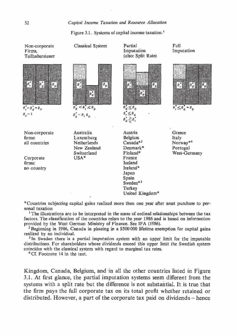
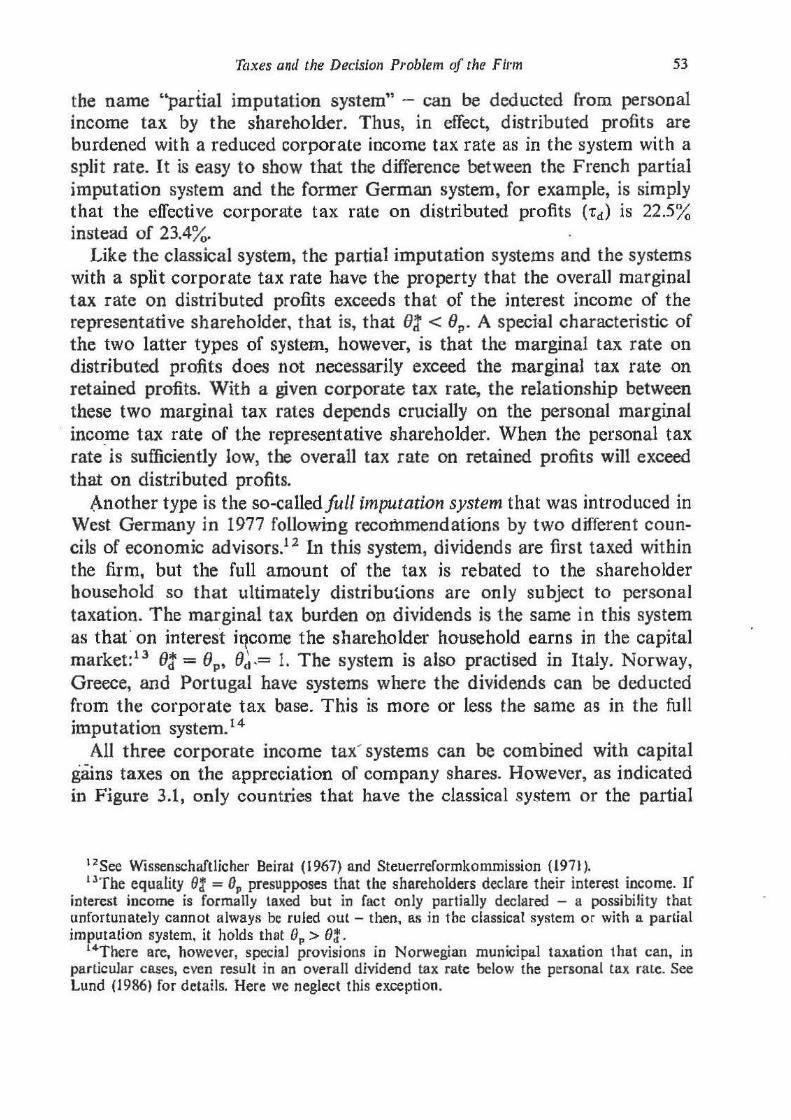
With the tax rates TP, -z:d, 1:ro and tc, from Equations (3.4)- (3.9) and (3.13), a general system of capital income taxation is described. If it is recalled that, by assumption, the tax rates refer to a representative firm and to a representative shareholder of this firm9 then some basic types of existing systems of capital income taxation or systems that have been discussed can be represented by this general system.1 ° Figure 3.1 iHustrates such basic types in that it depicts various ordinal patterns of the tax factors defined above. According to the three elementary types of capital income -retentions, dividends, and interest income - the presentation concentrates on the tax factors ()~, o:, and OP that measure the o.;verall tax burdens on these income categories. ~

The simplest system is one where. there are no capital gains taxes and the marginal tax rates on all three kinds of capital income are equal. It is realized in the sector of non-corporate firms since, with a non-corporate firm, the taxation of profits is determined solely through the personal income tax of the owner of the firm; there is no corporate income tax and wealth increases from an investment of taxed profits are tax exempt. Whether the owner of a non-corporate firm decides to invest an additional dollar of profit in his own firm, to consume it, or to invest it in the capital market, the returns in each case are subject to the same tax rate. Thus it holds that B: = 8~ = BP where Be = Od = 1.

In the industrial countries of the Western world, however, a significant section of the economy- in the United States, for example, about 85%- is

8 Cf. the discussion of Equation (3.21) below. 9 As far as corporations are concerned, the representative shareholder is the shareholder who

has the median position with regard to the distribution of personal marginal income tax rates among the set of company shares (not among the set or shareholders). Thus, the representative shareholder is the one who decides on the policy of the firm when there is majority voting. If there are other voting rules, for example with non-corporate firms, the representative sharehol­der is at any rate the person who ultimately determines the firm's policy. This definition does not exclude the set of shareholders belonging to .a company depending in turn on this company's financial policy (clientele effect).

10 Other categorizations can be found with Mennel (1971), FHimig (1974, pp. 56-63), King (1977, pp. 50-58), and in the information bulletin of the W11st German Ministry of Finance, for example. (See IFA 1986). Cf. also Musgrave and Musgrave (1973, Chapter 12), Wohe (1978, Chapters II and Ill), Boadway (1979, Chapter 13-4), or Fullerton/King (1984).

Taxes and .the D~cision Problem of tile Finn 51

or:ganized in the form of corporate firms and is thus subject to corporate income taxation. In principle it would not be difficult to design the corporate income tax so that the tax factors are equal for all three types of capital income. It would be necessary for this purpose to atttibute all parts of the accounting profit, even the retained profit, to the single shareholders and then to apply their personal income tax rates. This idea was proposed by the Carter Commission (1966). It is also central to the so­called Teilhabersteuer suggested by Engels and Stiitzel (1968), and goes back to Goode (1947) and to Dietzel (1859).11 Up to now, however, no country has managed to struggle through to the Tei"Ihabersteuer. The retained profits of the corporate firm, at least, are taxed everywhere without considering the personal aspects of the shareholder. The equality of all three tax factors is nowhere realized.

The systems of capital income taxation that are realized in practice can basically be reduced to three different types.

The first type denotes the so-called classical systent of capital income taxation. All profits, whether retained or distributed, are burdened with a uniform corporate income tax rate. In addition, distributed profits are subject to personal income tax and so too is interest income earned .in the capital market. In this system, (Jd = (Jr and so the effective tax factor for a unit of distributed profits is o: = (Jr(Jp· Because of the double taxation it falls short of both the tax factor for retained earnings and the tax factor for interest income of households.

The classical system was practised in the United Kingdom, Denmark, Germany, and many other countries, but today it seems a little less fashionable. It only exists in the United States and in a number of smaller countries some of which are listed in Figure 3.1.

The second type inc1udes systems with partial imputation and others with a split corporate tax mte without imputation of the corporate tax to the personal income tax. The system with a split rate was employed in West Germany from 1953 until 1976. After 1958 the tax r_ate for retained profits was 51%. Distributed profits were first tax~ at an effective corporate tax rate of 23.4% and then, a second time, at the personal income tax rate. Currently, among the countries listed in Figure 3.1, only Austria employs the system with a split rate.

Partial imputation systems are in use in Japan, France, the United

1 1 The verbal translation of "Teilha bersteuer'' is ''partnership tax" but "integrated tax'' might be a translation that better describes its essence. [Goode is cited according to Carter Commission {1966, Chapter 19, p. 94) as I was unable to get the article; the author.]

52

Non~corporate

Firms, Teilhabersteuer

N on·cor por ate firms: all countries

Corporate firms: no country

Capital Income Taxation and Resource Allocation

Figure 3.1. Systems of capital income taxation. 1

Classical System

Australia Luxemburg Netherlands New Zealand Switzerland USA*

Partial lmpu.tation (also: Split Rate)

Austria Belgium Canada*2

Denmark* Finland* France Iceland Ireland* Japan Spain Sweden"' 3

Turkey United Kingdom*

Full Imputation

Greece Italy Norway*4

Portugal West-Germany

*Countries subjecting capital gains realized more than one year after asset purchase to per­sonal taxation

1 The illustrations are to be interpreted in the sense of ordinal relationships between the tax factors. The classification of the countries refers to the year 1986 and is based on information provided by the West German Ministry of Finance. See IFA (1986).

2 Beginning in 1986, Canada in phasing in a $500 000 lifetime exemption for capital gains realized by an individual.

3 In Sweden there is a partial imputation system with an upper limit for the imputable distributions. For shareholders whose dividends exceed this upper limit the Swedish system coincides with the classical system with regard to marginal tax rates.

4 Cf. Footnote 14 in the text.

Kingdom, Canada, Belgium, and ·in all the other countries listed in Figure 3.1. At first glance, the partial imputation systems seem different from the systems with a split rate but the difference is not substantial. It is true that the firm pays the full corporate tax on its total profit whether retained or distributed. However, a part of the corporate tax paid on dividends- hence

Taxes and the Decision Problem of the Fit·m 53

the name '"partial imputation system" - can be deducted from personal income tax by the shareholder. Thus, in effect, distributed profits are burdened with a reduced corporate income tax rate as in the system with a split rate. It is easy to show that the difference between the French partial imputation system and the former German system, for example, is simply that the effective corporate tax rate on distributed profits (td) is 22.5% instead of 23.4%.

Like the classical system, the partial imputation systems and the systems with a split corporate tax rate have the property that the overalJ marginal tax rate on distributed profits exceeds that of the interest income of the representative shareholder, that is, that e: < 8P. A special characteristic of the two latter types of system, however, is that the marginal tax rate on distributed profits does not necessarily exceed the marginal tax rate on retained profits. With a given corporate tax rate, the relationship between these two marginal tax rates depends crucially on the personal marginal

· inco_me tax rate of the representative shareholder. When the personal tax rate is sufficiently low, the overall tax rate on retained profits will exceed that on distributed profits.

Another type is the so-called full imputation system that was introduced in West Germany in 1977 following recommendations by two different coun­cils of economic advisors.12 In this system, dividends are first taxed within the firm, but the full amount of the tax is rebated to the shareholder household so that ultimately distributions are only subject to personal taxation. The marginal tax burden on dividends is the same in this system as thaf on interest iq.come the shareholder household earns in the capital market:13 e: = (JP' 0~,= 1. The system is also practised in Italy. Norway, Greece, and Portugal have systems where the dividends can be deducted from the corporate tax base. This is more or less the same as in the full imputation system.14

All three corporate income tax' systems can be combined with capital gains taxes on the appreciation of company shares. However, as indicated in Figure 3.1, only countries that have the classical system or the partial

12See Wissenschaftlicher Beirat (1967) and Steuerreformkommission (1971). I 3The equality 9£ = ep presupposes that the shareholders declare their interest income. If

interest income is formally taxed but in fact only partially declared - a possibility that unfortunately cannot always be ruled out- then, as jn tbe classical system or with a partial imputation system, it holds that op > o:.

14There are, however, special provisions in Norwegian municipal taxation that can, in particular cases, even result in an overall dividend tax rate below the personal tax rate. See Lund (1986) for details. Here we neglect this exception.

54 Capital Income Taxation and Resource Allocation

imputation system tax capital gains realized more than one year after asset purchase. This seems consistent in so far as double taxation of distributed profits is complemented by double taxation of retained profits.

Even in countries where all capital gains are taxed, the tax rate is typically less than the tax rate on the interest income of a shareholder household: Be > OP. There are two reasons for this. On the one hand, it was agreed to utilize an equivalent capital gains tax rate on accrued capital gains that, as explained, falls short of the rate on realized capital gains which is stated in the tax law. On the other hand, even the legal tax rate is typically lower than the marginal person'al income tax rate as realized capital gruns are only partially included in the personal tax base when the speculation period has elapsed.

A ·somewhat peculiar situation prevails in the United States. Here, only 40% of realized capital gains used to be included in the tax base if the realization occured more than half a year after the shares were purchased. With reference to a study by Bailey (1969), Fullert6,n et al. (1981, p. 684) have estimated that the equivalent capital gains tax' rate of a shareholder was only one quarter of this marginal personal tax rate ( 't"c ~ 0.25 't"p).

However. the 198,6 tax reform changed the situation by expanding the speculation period to infinity: from 1988 onwards, realized capital gains will be fully subjected to personal income tax, regardless of the time span between the purchase and sale of the asset. Only the first reason for ec > ep will therefore be operative in the United States. It is not clear precisely how this will affect the equivalent tax rate on accrued capital gains. There are counteracting effects in that, on the one hand, the average period of asset holding will probably fall and, on the other hand, not all capital gains are affected by the doubling of the tax base. Nevertheless, a good guess might be that, relative to the personal tax rate, the equivalent capital gains tax rate will be about two and a half times its pre-reform value; that is, about sixty percent of the personal tax rate: 't"d ~ 0.6 rP. ·

The classical system is characterized by Bd' = erep. Thus the preferential treatment of capital gains relative to interest income implies that, in this system, the combined tax factor for retained profits exceeds the combined tax factor for distributed profits: fJ~ = Or:er > o:. With the partial impu­tation systems, on the other hand, the ambiguity with regard to the relative magnitudes of f)r and Oj carries over to Oi and Oj. With a high degree of imputation of dividends and a high capital gains . tax rate. even the case Ot < o: would be possible here.

Despite all the differences between the various systems -of capital income taxation, they have two characterjstics in common. These should be stressed

Taxes and tl1e Decision Problem of rlre Fil"m 55

here since they are, as will be shown, quite important for the working of the capital market. The first characteristic is that the marginal personal tax rate of the representative shareholder household lies between the marginal combined tax rate on distributed profits and the marginal tax rate on capital gains:

(}* < 0 < ll d - p - uc. (3.14)

The first part of this inequality follows from the fact that, in all systems, dividends are fully subject to personal income tax and, in most systems, are also subject to corporate income tax, either fully or partially.15 The second part follows from the fact that realized, and not accrued, capital gains are subject to personal income taxation, typically even at less than 100%.

The second characteristic refers to t,he relative magnitude of the direct and indirect tax burden on retained profits on the one hand and the tax burden on the interest income of the representative shareholder household on the other. While the previous discussion has shown that non-corporate firrris are characterized by Bi = fJP the relationship between these tax factors is more ambiguous for corporate firms. In countries where the maximum m~rginal personal tax rate exceeds the corporate tax rate and where there is no capital gains tax, fJP can either exceed or fall short of 8~, depending on the tax bracket of the representative shareholder household. There are, however, certain indications that

e: < ep (3.15)

(or even 8~ ~ fJp) characterizes the normal case. First, in countries like Canada, Denmark, or West Germany, the pro­

gression of the personal income tax scale stops at the level of the corporate . tax rate or even below. In these countries, the case e; >BP can be excluded

right away. Secondly, in about half of the countries- among them the United States,

Australia, and a number of European countries - the corporate tax rate on retained profits is more than three quarters of the maximum personal income tax rate.16 In these countries, too, the case 8': >BP does not seem to be very plausible for the representative shareholder. that is, for that

15Cf. the previous footnote. 16 In 1986, 13 out of24 OECD countries (eKcluding Yugoslavia) satisfied this criterion. The

national product of these 13 countries amounts to more than t 60% of aggregate OECD national product. See IFA (1986, Obersicht 1 and 4), ITS (1985}, and Weltbank (1985, pp. 202 n.).

56 Capital Income Taxation and Resource Allocation

shareholder who occupies the median position with regard to the distri­bution of marginal personal tax rates.

Thirdly, in contrast to the direct check on retained profits of corpo­rations, governments seem to have substantial difficulties in monitoring the interest income earned by households. It is well known that in a number of countries only a small percentage of interest incomes is actually taxed. Thus, even if ()~ > (JP were the case when tax payers are honest. ()~ <Bp could be the case when they are not.17

Fourthly, the capital gains tax that is levied in the eight countries denoted by an asterisk in Figure 3.1 supports Condition (3.15). Consider for example the United States. With the post-1986 corporate tax rate of tr = 0.34 that applies to most firms and the cited value of the equivalent tax rate of re :::e 0.6 rP on accrued capital gains, it follows from the condition (1 - 'tr) (I - re) = 1 - rP that the critical value for the marginal personal tax rate of the representative shareholder is rP = tr / [1 - (Or· 0.6)] :::e 0.56. If the true value of TP is on or below this level then Condition (3.15) is satisfied, and this is indeed the case. The U.S. income tax reform of 1986 reduced the maximum marginal rate of federal income tax from 501}1~ to 33%, and state income taxes are normally not more than 12% of income net of the federal tax. 18 These pieces of information together imply that the upper limit of the overall marginal personal tax rate is 41% - a value far below the critical value.19 The federal rate of 33% only applies to a limited income range though. Most shareholders, including very rich ones, will pay a marginal federal tax rate of 28~1~. This reduces the upper limit of the sum of the marginal state and federal rates to about 371% which is even further below the critical value.

Before the 1986 tax reform, the situation in the United States was more ambiguous. During this time, the corporate tax rate was 46% for most corporations and so the value Tc = 0.25'tp calculated by Fullerton et al. implies a critical value for the marginal personal tax rate of Tp = tr/[1 - (8r·0.25)] ~ 0.54. With a top federal income tax rate of 50% (70% before 1981), the sum of the marginal state and federal income tax rates in principle could exceed this critical level. On the other hand, in many

1 7 There is no monitoring problem in countries like the United Kingdom or Sweden since these have source taxes on interest income. However, the .tax rates are far below the respective corporate tax rates.

18 See ITS ( 1985, Section U-28}. 19 T o be on the safe side this calcu1ation neglects tbe state corporation franchise taxes and

the additional 5% corporate tax charged to phase-out the benefit of graduated rates for small corporations. To include these taxes would mean raising the critical value, and (3.15) would hold for an even stronger reason.

Taxes and the Decision Ptoblem of the Firm 57

cases the representative shareholder's marginal personal tax rate was cer­tainly below the top rate. As Bradford (1980, pp. 51, 55) reports, the U.S. treasury estimated that the average marginal personal income tax rate of shareholders was 40% in the year 1976. Although the average shareholder cannot necessarily be identified with the representative shareholder, this suggests that there may not have been many firms for which Condition (3.15) was violated.

Despite these arguments, empirica-l grounds cannot provide sufficient support for Condition (3.15) in the case of each and every firm and country. In Japan, the United Kingdom, France, Italy, Spain, and a number of smaller countries the maximum personal income tax rate exceeds the corporate tax rate sufficiently far to make the case 6:' > f)P appear possible or even plausible for many firms. There are however, in addition, two theoretical arguments in favor of Condition (3.15) that will be discussed in Chapters 4.2.2 and 4.3.4. One is Miller's. (1977) argument that firms will adjust their debt- equity ratios to the point where, because of the progressivity of marginal personal tax rates, (3.15) holds with equality (e: =Bp). The other is based on the non-existence of an intertemporal gt?neral equilibrium with e: > eP. These theoretical arguments perhaps support Condition (3.15) even more strongly than the empirical evidence.

3.1.3. The Possibility of Accelerated Tax Depreciation

With Equations (3.3.) and {3.4) it was assumed that, for the calculation of taxable retentions, true economic depreciation of the capital stock is allowed, that is, a depreciation that reflects the true loss in market value (bK) of the capital stock employed. These equations therefore correspond to the Schanz-Haig-Simons definition of income which might have been the ideal that lay behind the construction of the income tax systems of the Western industrial nations.

It should be legitimate, to a first approximation, to use this ideal for an analysis of tax effects in some countries. Perhaps West Germany is such a country for, according to a study by Kopits (1975, p. 33), except for Luxembourg, it seems to be the most restrictive of all OECD countries in its depreciation allowances. However, it should not be overlooked that the attempt to formulate tax depredation rules in line with true economic depreciation is, in the international context, more the exception than the rule. With the passage of time, many countries have significantly loosened their depreciation rules, and for a while some of them seemed to be no

58 Capital Income Taxation and Resource Allocation

closer to true economic depreciation than to an immediate write-off. The United Kingdom and the United States in particular had, and

continue to have, quite generous depreciation systems.Z0 Until 1984 the U.K. allowed a 75% depreciation of industrial buildings in the first year and straight line depreciation thereafter. Plants could even be written off at a rate of 100% in the first year. From 1986 onwards there are no longer any initial depreciation allowances. However, a declining-balance depre­ciation for plants at the high rate of 25% p.a. remains. Only a little less generous than the previous Briti.sh depreciation rules were those that the United States introduced in 1981 under the Reagan administration with the so-called Accelerated Cost Recovery System (ACRS). According to this system, the majority of plants could be fully depreciated over as few as five years. 21 H was estimated that by 1;he year 1986 when the new rules should have been fully operative, there would have been a loss in tax revenue of between $54 and $61 billion - figures that hav,e the same order of magnitude as the total U .S. corporate income tax ievenue in 1981.2 2 The expected revenue losses were so dramatic that the Reagan administration took fright and abolished, as a first reaction, the generous "safe-harbor leasing" arrangements for inter-firm loss transfers that had come with the reform and that were being intensively exploited by industry. Shortly after the President was re-elected in f984, the Treasury even proposed returning to more conservative depreciation rules,23 and this proposal ultimately resulted in the U.S. tax reform of 1986. According to the new Jaw most plants can be depreciated in about 7 years. This is two years more than under ACRS, but still about three years less than under the Asset Depreciation Range System that preceded ACRS: It is certainly also less

·than the economic life of most plants.24

20 Other examples with generous depreciation systems include Canada and Australia, where plant is usually eligible for a depreciation period of not more than five years. By contrast, depreciation periods for plant in West Germany try to approximate "economic useful life" which is significantly more than 10 years. Cf. Footnote 24.

21 Exceptions were buildings that could be depreciated over 15 years and short-lived assets like automobiles that could be depreciated over three years.

22See U.S. Joint Committee on Taxation (1981, Table 2, p. 58) and the table "Changes in Fiscal Year Receipts Resulting from the Conference Agreement on H.R. 4242, the Economic Recovery Tax Act of 1981, Office of the Secretary of the Treasury, Office of Tax Analysis, August 3, 1981" that was issued by the the U.S. Department of the Treasury. For the American· corporate income tax revenue compare, for example, Survey of Current Business 64, 1984, Table S-14, where a corporate tax revenue of $61.137b. in 1981 and a revenue of only $37.022 b. in 1983 is revealed. Cf. Auerbach (1982), Sunley (1982), and Sinn (1984b) for discussions of various economic effects of ACRS.

23 See U.S. Department of the Treasury (1984). 24 For West Germany, Jatzek and Leibfritz (1982, Table 5, p. 66) estimated an average life of

Taxes and the Decisio11 Problem of the Fi1·m 59

In the light Qf this information, the problem of accelerated tax depre­ciation can hardly be avoided in a realistic analysis of tax distortions, and the question arises of how the phenomenon can be formally represented. Despite certain differences in the depreciation allowances in the various countries, there are three aspects that are typical. First, because of the interest advantage of accelerated depreciation, the profitability of invest­ment projects rises. Second, hidden reserves are created. With accelerated depreciation, the tax-written-down value of the capital stock falls short of the market value of capital, and the difference between these values is a reserve that is hidden from the tax balance sheet.25 Third, the sum of tax depreciation allowances calculated for the total life span of an asset equals its initial purchasing value. All these aspects should be taken into account in the formula!jon of an _ll .. m~ropria.te..Jn..Q.del_. ,_ --· ...... . . .. ..... . .. ..... ... _ .. _ . __ _ ·-

----A way of modelling accelerated depreciation that seems attractive at first sight consists of the assumption that, at each point in time, tax depreciation exceeds true economic depreciation by a certain percentage. This assum­ption takes the first of the three aspects into account, but not the other two. The total volume of tax depreciation is more than 100% of the initial purchasing value of the equipment. and there are no hidden reserves. Thus, another, equally simple and quite familiar assumption will be made here.

It is assumed that a certain proportion a 1, 0 < a1 < 1, of an investment expenditure is depreciated immediately and the remainder 1 - a 1 gradually over time by keeping the tax depreciation at a level of 1 - C(1 times true economic depreciation. Since, at each point in time, gross investment is I + ~K, and since true economic depreciation is oK, the flow of immediate depreciation on new investment is lX1 (I + bK) and the flow of depreciation on existing assets is (1 - adc5K. Hence, the aggregate current flow of tax depreciation is26

(3.16)

It consists of true economic depreciation plus the proportion o: 1 of net investment. The formula for the revenue from taxing retained profits

13 years for plants expiring at the end of the seventies. ln the presence of inflation and historical cost accounting_ a somewhat shorter depreciation period than this would be necessary to approximate true economic depreciation. According to the U.S. Department of the Treasury (1984, pp. 106 n.), the Asset Depreciation Range System can be seen as an attempt to be such an approximation.

25 Cf. Section 3.2.2. for further details. 26The analysis abstracts from the possibility or diverging depreciation rules for existing and

new assets. None of the allocative results derived in this book depends on this specification; only the tax treatment of new assets matters.

60 Capital Income Taxation and Resource Allocation

changes accordingly from (3.4) to:

Tr = -rr[f(K, L) - Tk - wL- oK- rDr- cx 11- lld]. (3.17)

The tax-written-down of the capital stock is (1 - ~tdK, and the value of the hidden reserves is K- (1 - cxx)K = ~t 1 K.27

Admittedly, the specification of the depreciation problem chosen cannot claim full generality. The assumptions that economic depreciation can be modelled as declining balance depreciation and that accelerated tax depre­ciation can be represented as a linear combination of economic depreciation and an immediate write-off clearly cannot do full justice to all aspects of depreciation that are relevant in practice. However, these assumptions are nevertheless flexible enough to capture the incentive effects relating to depreciation and, in fact, it is not difficult to translate the rules accountants use into the parameters of the model so as to produce an equivalence in present value terms. Suppose, using the discount rate i, the present values y 1

and y2 of economic and tax -depreciation have been calculated from empirical data. Then, equating the present value of declining balance . depreciation, 8/(i + 8), with the present value of economic depreciation, y 1 ,

gives 8 = iyd(l - yt}, and it follows from y 2 = cx1 • 1 + (1 - cxdy1 that cx 1 = (y2 - yx)/(1 -yd. Assume, for example, the American Asset Depreciation Range System, which was in operation before 1981 and allowed plants to be depreciated in about 10 years on average, can be associated with true economic depreciation. For discount rates between 3% and 10% and assuming straight-line depreciation, it then follows from these equations that 0.21 ~ o < 0.22 and that a reduction of the depreciation period fron ten to five or seven years increases the depreciation parameter cx 1 from zero to a value in the range 0.49 < cx1 -~ 0.53 or 0.25 < cx 1 < 0.32, respectively. As stylized facts it can therefore be assumed that the 1981 introduction of the Accelerated Cost Recovery System increased the depre~ ciation parameter a 1 from zero to about 0.5 and that the 1986 reform pushed this parameter back to a value of about 0.3.

21 Since Equation (3.17) is algebraic and hence includes arbitrary negative values of taxable retained profits, it implicitly allows ror a perrect loss-offset. This possibility is obviously unrealistic. It is true that many countries offer generous possibilities ror carrying loss rorward and backward and, as mentioned, for a while the United States even allowed for inter-company transfers of depreciation allowances. However, all of this by no means amounts to a perfect loss-offset. For this reason, Chapter 5 will study a special constraint on the financial planning of firms that allows for a temporary loss-offset but requires that the revenue from taxing retained and distributed profits be non-negative in a steady state. For the time being though we exclude the problem.

Taxes and the Decision Problem of the Finn 61

3.1.4. Alternative Assumptions on the Deductibility of Interest Costs

True economic depreciation and deductibility of debt interest are the basic ingredients of the Schanz-Haig-Simons concept of capital income taxation. A variation of this concept using different depreciation rules has been discussed. In addition, alternative assumptions on the deductibility of interest costs will now be considered.

On the one hand, a v~riable proportion ct3 (a3 = 0, a3 = 1) of non­deductible debt interest is to be allowed that can obtain values of either zero or one. On the other hand, it is assumed that a proportion a2 , again either with a value of zero or one (a2 = 0, a2 = 1), of the total, that is actual and imputed, interest cost rK can be deducted from the tax base of the firm. Utilizing the extension introduced with (3.17), the general version of the tax function (3.4) for retained profits can therefore be written as

This formulation is flexible enough to capture many different kinds of tax model

Only four classes of models will be treated in this book though.28 Not all variants of these classes will be discussed - ir only because existence problems require a limitation of possible parameter constellations in the case of non-deductible debt interest. However, variants that do not belong to one or other of these classes can already at this stage be definitely excluded from the ~nalysis.

(1) eP < 8c, a2 = cx3 = 0. This class includes all empirically relevant tax systems. Because of (3.14) and (3.15) the direct marginal tax burden on interest income, retained profits, and dividends is strictly greater than the effective marginal tax burden on accrued capital gains. The depreciation rules are arbitrary and only actual interest cost is deductible.

(2) (JP = ec. ('Xl = ()!2 = rt3 = 0. This constellation resembles Class (1); but it says that uniform taxation of interest income and accrued capital gains with full deductibility of actual interest cost is only examined in the context of true economic depreciation.

(3) cx1 = 0, a2 = cx3 = l. While the tax rates can have arbitrary values

28The basic assumptions (3.J4), (3.15); o~e1 ~l,j=d, r, p, c; O~a 1 ~1 ; a2 =0 or a 2 = 1; a3 = 0 or a 3 = 1 hold for all classes and are not repeated here.

62 Capital Income Taxation and Resow·ce Allocation

and true economic depreciation prevails, it is assumed that imputed and actual interest cost is deductible.

(4) a 1 = 1, a2 = 0, a3 = 1. This case characterizes an immediate write-off and a non-deductibility of interest costs of any kind. Again the tax rates are arbitrary.

The reason for considering alternative possibilities for deductibility of interest cost is not that, in practice, the taxation of firms deviates signi­ficantly from the Schanz-Haig-Simons concept. Indeed, actual interest cost, and only actual interest cost, can be deducted from the tax base by firms in all OECD countries. Rather, this general formulation serves the purpose of understanding the importance of the Schanz-Haig-Simons concept and, in particular, of examining different proposals for a reform of capital income taxation. .

Unlike the treatment of debt interest at the firm level the treatment of personal debt interest at the household level devili\tes from the Schanz-· Haig-Simons concept in some countries. While 1interest earned by a household is always taxable, debt interest paid by a household can some­times only to a limited extent be deducted from the personal tax base and sometimes not at all. We forego an explicit consideration of this aspect since it will turn that it is quite meaningless, in the framework of the present model, as long as the household possesses a strictly positive stock of tradable private assets and government bonds. Compare, in this context, the discussion of the borrowing constraint of private households in Chapter 8, Equations (8.12) and (8.53) through (8.55).

3.2. Tlhle OJpntimizmtiol!ll Pa·olb~em of tllne Fnll'm llm«ilen· tllne ll!llJ!llnnel!llce of Tmxmtim1

After considering various tax systems, the discussion can now turn towards the role of taxation in the decision problem of the firm. For this purpose it is useful to refer to the laissez-faire model of the firm formulated in Chapter 2.3. Unless otherwise indicated, all assumptions and definitions made there are maintained. The following remarks concentrate on a discussion of those aspects of the model that will alter under the influence of taxation.

3.2.1. The Market Value of Shares

As in the faissez-faire model, Fisher's separation theorem again implies that the firm tries to maximize the wealth of its representative shareholder and

Taxes and rhe Decision Problem of the Firm 63

hence the market value of its equity independently of the shareholder's specific preferences.29 Differently from before, however, various taxes have now to be taken into account.

First, those taxes must be considered that reduce the net flow of funds to the household. Because of (3.13) this net flow has the magnitude

n~ - Q - -r c( M ~ Q),

where n~ indicates net dividends.30 Net dividends are defined as dividends after all taxes including the personal taxes paid by the representative

. shareholder. How these taxes affect the size of ll~ will be explained in the next section.

In addition to the taxes that reduce the firm's profit, taxes on alternative investment opportunities are of crucial importance for its decision problem. According to (3.7), the interest income which the representative household earns from a capital market investment is subject to a marginal personal tax rat~ of size 'I'p· Thus the household's possibilities for an intertemporal transfer of consumption are described by the net-of-tax market rate of interest 8Pr. Hence this rate of interest is the discount rate for calculating the present value of the funds flowing from the firm to the representative household. It has to be stressed that the net market rate of interest is not defined with regard to that tax rate which applies to a capital market investment of thejirm.31 It is true that the tax rate on retained profits will indeed enter the marginal condition for optimal investment, i.e., that it will affect the discount rate which the firm uses for evaluating its investment projects. This discount rate, however, is yet to be derived from the optimization problem of the firm. Thus, instead of the laissez~faire equation, (2.3), we get the following expression for the market value of shares:

M(t) = r {ll~(v)- Q(v)- <,[M(v)- Q(v)] ) [exp f -llpr(s)ds ]dv. (3.19)

29 Cf. Footnote 12, Chapter 2. 30 ln contrast to Chapter 2, for the time being control variables of the firm will not be

indicated by a superscript ''u''. Only with the analysis of the intertemporal general equilibrium in Chapter 8 will this custom be taken up again to distinguish between the firm's and the household's control variables.

31 Some theoretical studies that do not distinguish between different kinds of marginal tax rate seem to be intended to apply to the marginal tax rate on the returns from capital market investments that the .firm receives. An example of a study where this is explicitly assumed is the paper or Hall and Jorgenson (1971, p. 16). The problem is related to the discussion about the so·called gl"oss or net interest assumption in the finance literature. Cf. e.g. Wohe (1965, pp. 198- 213). Buchner (1971, pp. 672--674), or Strobel (1970, pp. 382-384).

64 Capital Income Taxarion and Resource Allocation

In order to justify this expression on economic terms and to transform it into an equivalent expression that is easier to use, it can be differentiated with regard to time. The result is

M= - ll! + Q + t 0 (M - Q) + OprM (3.20)

or, with consideration of the relationship M= mz + zm:

II~ + rhz9c + (im - Q)Oc = OprM. (3.21)

This equation describes a requirement that the development of the market value has to satisfy if there is to be an arbitrage equilibrium between investment in shares and bonds. It could have been used instead of (3.19) as a starting point for deriving an expression for market valuation. In order to make wealth owners indifferent between retaining shares at a value of M or exchanging these shares for bonds, the current net return on shares has to outweigh the potential net returns ()PrM from holding bonds. The net return on shares is represented by the lefthand side of the equation and consists of three components. The first is the current net dividend paid out to shareholders, Il~. The second is the capital gain mz6c from the existing stock of shares net of the capital gains tax. The third is the net~of~tax capital gain (im- Q)Oc from issuing new shares at a price below their market value.

This last component is not necessarily important in countries like the United States since existing shareholders will object to a policy of diluting their assets and will require that im = Q. The situation is different, however, in other countries - an example is West Germany - where new shares cannot be issued without providing the existing shareholders with tradable purchasing options. If purchasing options are distributed, existing share­holders will not necessarily object to selling the shares at a price below the stock market value since any difference creates an option value of equal size that they can realize in the market place without even buying the new shares themselves. The value of the purchasing options is im - Q, and, in principle, it is subject to the capital gains tax. Clearly the net-of-tax value of the flow of purchasing options provided to the existing shareholders contributes to the return from holding shares and has to be included in the arbitrage condition (3.21). 32

The market value function (3.19) from which the arbitrage condition (3.21) was derived is quite clumsy for certain mathematical operations since

32Cf. Aktiengesetz (1955, §186) for further institutional details of the regulation in West Germany.

Taxes and the Decision Pl'oblem of the Fil'm 65

within the integral on the righthand side the derivative of the same integral, M, appears. This problem can be avoided if (3.20) is solved for M and the resulting differential equation

. n~ op M=--+ Q +--rM

()c e .. {3.22)

is integrated, an operation that is just the reverse of the step from (3.19) to (3.20). Under the existence requirement

[(lld(t) ) f' () J !~~ 0c - Q(t) exp

0 - o: r(s) ds = 0 (3.23)

one obtains33

ia:>(lld(v) )( iv () ) M(t) = -t--Q(v) exp 1

- e: r(s) ds dv. (3.24)

This formula for the market value of shares is completely equivalent to Equation (3.19). It shows that there is an alternative to deducting the capital gains tax from the current flow of funds from the firm to its shareholders. This alternative is to divide the net dividends and the net market rate of interest, but not the value of the current flow of new shares, by the capital gains tax tfactor Oe.34 Because of its analytical simplicity, only (3.24) will be used in \the analysis.

33 It is assumed that the market value is zero if the firm never issues new shares and never pays out any dividends. Hence the integration constant is set equal to zero. Note that allowing for a non-zero integration constant would not affect the solu.tion of the optimization problem (3.29).

34For the case without new issues of shares (Q = 0), (3.24) resembles an expression derived by King (1974a. p. 23) in discrete time. Moreover, in the special case where new shares are issued at their market value that is, in the case where the value of the purchasing options given to the existing shareholders is zero (im = Q) the formula is compatible with the market value function

M(t) =f.~ [ll~(v)- -r.,m(v)z(v)]{ exp r- [Opr(s) + !5*{s)]ds} dv, b*sQ/M.

This can be shown if this function is differentiated for t and the resulting expression mz + im = -R0 + -r: 0 1tzz + 9PrM + Q is transformed into a version that corresponds to (3.21}. The discrete-time analog of this funclion is used by Auerbach (1979a) who, however, uses a debt­determined discount rate rather.-than the net market rate of interest. A similar expression can also be found in a paper by Poterba and Summers (1983).

66 Capital Income Taxation and Resource Allocation

3.2.2. Definitional Relationships between Taxation, Accounting Profit, and Dividends

Following these theoretical preliminaries, this section has the task of clarifying some definitional relationships that will later be needed for calculating the optimal policy of the firm.

Consider first accounting profits whose definition is of particular impor­tance since, in all OECD countdes, they are an upper limit for the dividends of corporations. In the case of true economic depreciation in the balance sheets, the accounting profit differs from the laissez-faire accounting profit of Equation (2.1) only by the capital tax and is defined by Equation (3.3).

With accelerated depreciation, however, the accounting profit may be smaller, depending on which accounting rules are used. This analysis is limited to the rules that are valid in the Anglo-Saxon countries since there, as explained above, accelerated depreciation seetn,s to be of particular importance. :

There are two distinct balance sheets, the tax balance sheet drawn up for the taxation department and the commercial balance sheet drawn up for the shareholders. Different values may be given to a firm's assets in these two balance sheets. Accelerated tax depreciation has immediate consequences only for the values appearing in the tax balance sheet. However, a potential tax on the reserves hidden· from this balance sheet has to be entered in the commercial balance sheet under the category deferred taxes. Given the depreciation formula (3.16), the current increase in the stock of deferred taxes is 1:,rx1J. Thus the current flow of net tax savings resulting from accelerated depreciation reduces the current accounting profit. 35 Accord­ingly, this accounting profit is

fl = f(K, L)- [JK- wL- rDr- Tk- t,rx 1J. (3.25)

The accounting profit is the legal source of the dividends which the firm can pay. Consider first gross dividends fld. In order to calculate them, the tax on retained profits (T,) and that part of net investment that cannot be financed through deferred taxes [1(1- rx 1t,)] have to be subtracted from the accounting profit, and the net inflow of funds from issuing bonds, Sr, and shares, Q, has to be added:

fld = fl + Sr + Q -1(1- rx 11:,)- T,. (3.26)

This equation differs from its laissez-faire counterpart (2.2) not only by the taxes but also by emphasizing new issues of shares as a source of finance.

35 Cf. Jung (1979, p. 121) or Alworth (1979).

Taxes and tlte Decision Problem of the Firm 67

In the laissezwfaire model! no particular attention was paid to this source of finance since it was agreed to consider negative values of dividends as new issues of shares. In the case of taxation this procedure is no longer admissible since, as already follows from (3.24), tax laws do not treat new issues of shares symmetrically with dividends.

Because of (3.5), the net dividends can be calculated from Equation (3.26) by multiplying with the tax factor e~ for distributed profits:

n d _ rn:t T* _ (}*fld n- u.-- d - d · (3.27)

Using (3.2), (3.18), (3.25), and (3.26), this expression can be transformed after a number of simple algebraic manipulatio~s into the equation

. e* ll~ = e:[J(K, L)- l>K- wL- rDr] +

8d. [Sr + Q- I] r

8* + 'rr f/ [cxtl + et. 2rK - IX3r·Dr]

r

(3.28)

The expression in the first line on the righthand side of (3.28) denotes the value of the net dividends for the case where taxes on retentions are calculated according to the initial formula (3.4) and where there are no indirect taxes. The expression in the second line shows the correcting terms that were introduced with (3.18). The expression in the third line measures the reduction in the net dividends through the tax on the capital stock.

3.2.3. The Formal Optimization Approach

Using the information given in Section 3.2.1 and 3.2.2, the structure of the optimization problem of the firm can easily be represented.

The firm faces given time paths {r} and {w} of the interest rate and the wage rate. It tries to choose the time paths of employment of efficiency units of labor {L }, net increase in debt {Sr }, new issues of shares { Q}, and net investment {I} so that the market value of its shares is maximized:

max M(O). IL,Sr.Q.T)

(3.29)

The state variables of the optimization problem are the capital stock (K)

and the stock of debt (Dr ). As in the laissez·faire model, the following

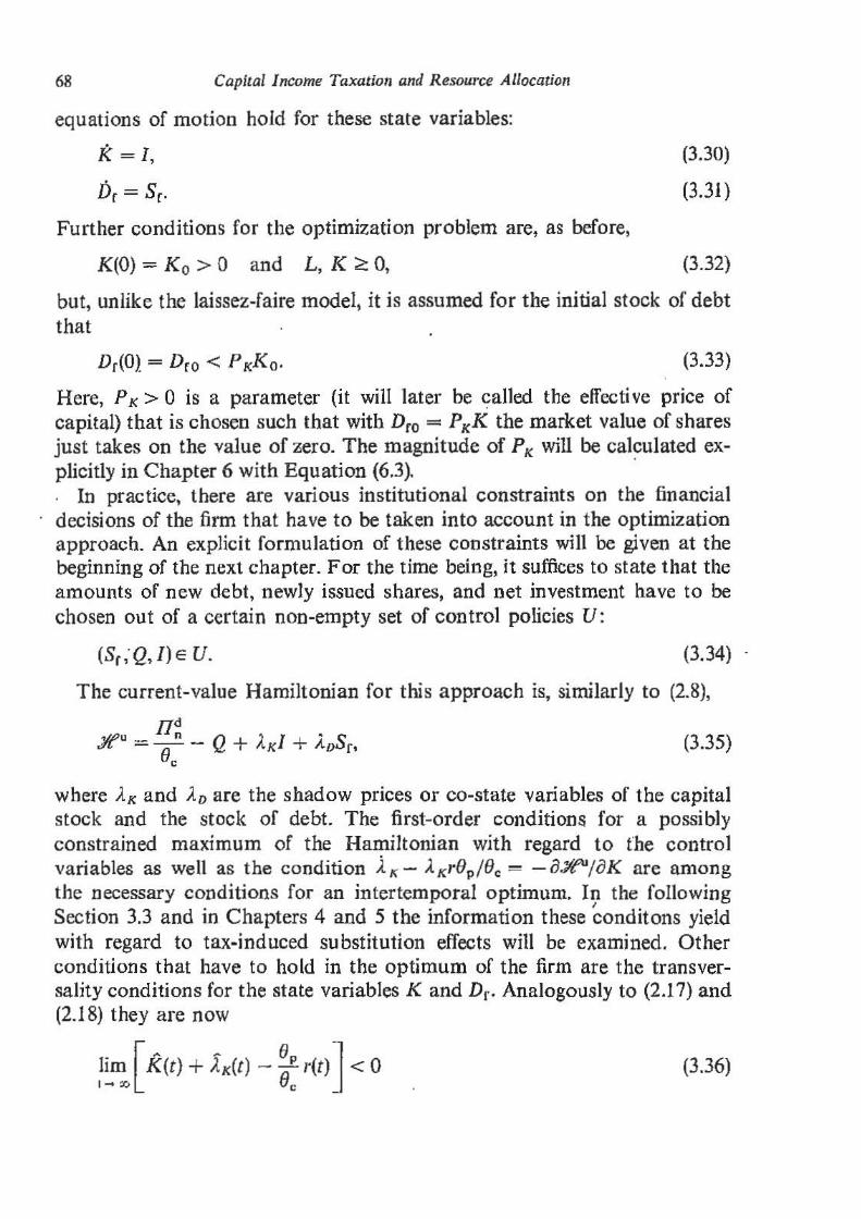
68 Capital Income Taxation and Resou1·ce Allocati(m

equations of motion hold for these state variables:

K =I,

Dr =Sr.

Further conditions for the optimization problem are, as before,

K(O) = K 0 > 0 and L, K ~ 0,

(3.30)

(3.31)

(3.32)

but, unlike the laissez-faire model, it is assumed for the initial stock of debt that

(3.33)

Here, P K > 0 is a parameter (it will later be <?alled the effective price of capital) that is chosen such that with Dro = PKK the market value of shares just takes on the value of JSero. The magnitude of PK will be calculated ex-plicitly in Chapter 6 with Equation (6.3). · . In practice, there are various institutional constraints on the financial decisions of the firm that have to be taken into account in the optimization approach. An explicit formulation of these constraints will be given at the beginning of the next chapter. For the time being, it suffices to state that the amounts of new debt, newly issued shares, and net investment have to be chosen out of a certain non-empty set of control policies V:

(3.34)

The current-value Hamiltonian for this approach is, similarly to (2.8),

.7/fu = ~~ - Q + }.KI + AoSr, c

(3.35)

where A.K and .:1. 0 are the shadow prices or eo-state variables of the capital stock and the stock of debt. The first-order conditions for a possibly constrained maximum of the Hamiltonian with regard to t'he control variables as well as the condition l K- A. K~'Op/(}c = - iJJit'UjiJK are among the necessary conditions for an intertemporal optimum. In the following

I

Section 3.3 and in Chapters 4 and 5 the information these conditons yield with regard to tax-induced substitution effects will be examined. Other conditions that have to hold in the optimum of the firm are the transver­sality conditions for the state variables K and Dr. Analogously to (2.17) and (2.18) they are now

[ ... ~ () J !~n; K(t) + ).K(t) - e: r(t) < 0 (3.36)

Taxes and the Deci.~ion Problem of the Fil"m . 69

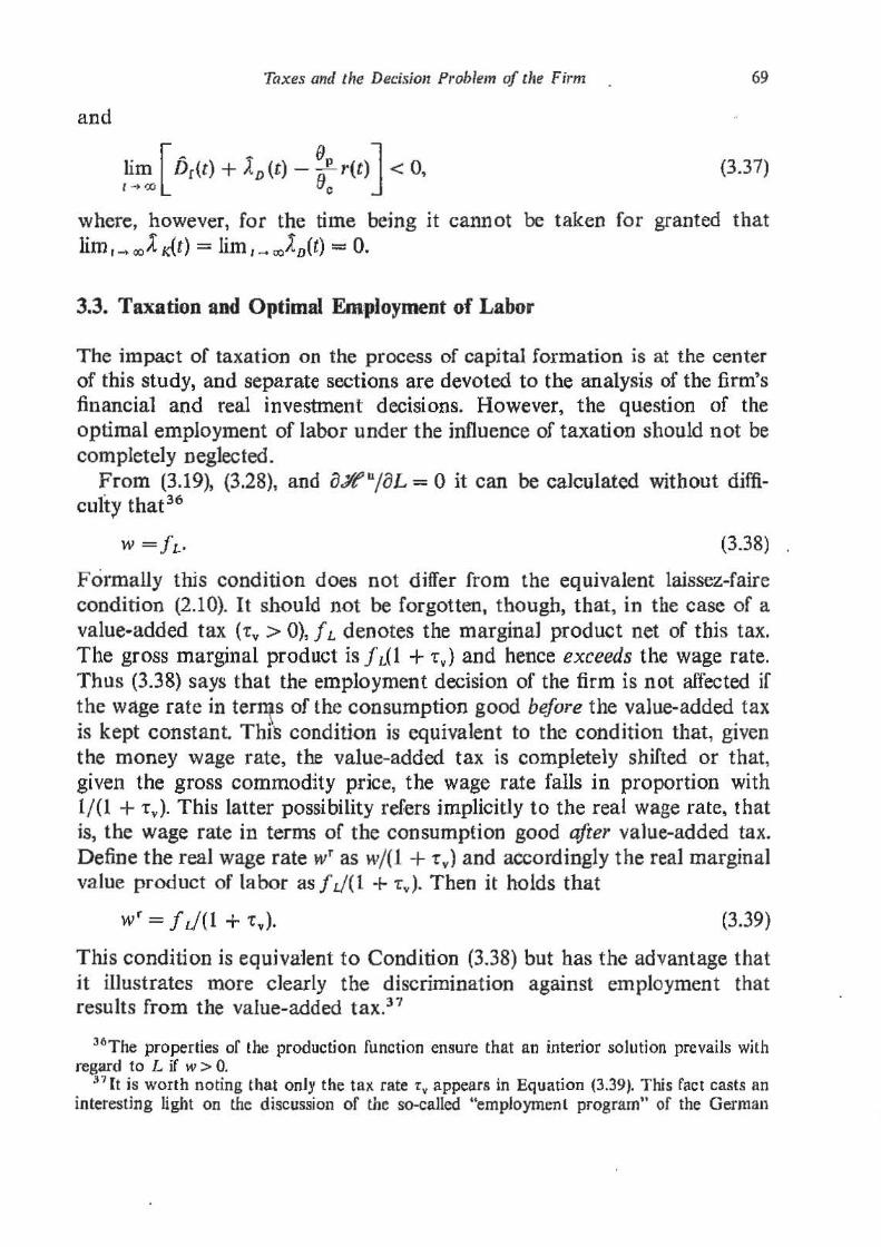
and

[ ~ - 9 J /1~~ Dr(t) + ), D (t) - a: r(t) < 0, (3.37)

where, however, for the time be:ing it cannot be taken for granted that lim ,_ ooA K(t) = lim , .... ooAD(t) = 0.

3.3. Taxation and Optimal Employment of Labor

The impact of taxation on the process of capital formation is at the center of this study, and separate sections are devoted to the analysis of the firm's financial and real investment decisions. However, the question of the optimal employment of Iabor under the influence of taxation should not be completely neglected.

From (3.19), (3.28), and o.YtujiJL = 0 it can be ca1culated without diffi­cufty that 36

(3.38)

Formally this condition does not differ from the equivalent laissez-faire condition (2.10). It should not be forgotten, though, that, in the case of a value-added tax (rv > 0), !L denotes the marginaJ product net of this tax. The gross marginal product is f dl + -rv} and hence exceeds the wage rate. Thus (3.38) says that the employment decision of the firm is not affected if the wage rate in ter:t~s of the consumption good before the value-added tax is kept constant. Thi's condition is equivalent to the condition that, given the money wage rate, the value-added tax is completely shifted or that, given the gross commodity pric.e, the wage rate falls in proportion with 1/(1 + rv). This latter possibility refers implicitly to the real wage rate, that is, the wage rate in terms of the consumption good after va1u·e-added tax. Define the real wage rate wr as w/(1 + rv) and accordingly the real marginal value product of tabor as f J(l + -rv). Then it holds that

wr = f d(l + rv). (3.39)

This condition is equiva·Ient to Condition (3.38) but has the advantage that it illustrates more cJearly the discrimination against employment that results from the value-added tax.3 7

36The properties of the production function ensure that an interior solution prevails with regard to L if w > 0.

37 [t is worth noting that only the tax rate 'rv appears in Equation (3.39). This fact casts an interesting light on the discussion of the so-called "employmenl program" of the German

70 Capital Income Taxation and Resource Allocation

It seems quite plausible, and does not require any additional explanation, that the taxation of the capital stock is unimportant for labor demand when the capital stock is given. The fact that the taxes on interest income and profit do not show up in (3.39) is not quite so self~evident.

The reason for the irrelevance of the taxation of the interest income of households is that the employment decision is~ in principle, a static optimi~ zation problem. It is true that the discount rate may change with the tax on interest income. However, the rate at which the marginal profit of the last worker employed at a particular point in time is discounted is completely unimportant. The present value of this marginal profit is zero in any case.

The reason for the irrelevance of the profit taxes has long been known in public finance:38 Since the profit from employing the marginal worker is zero, there is no tax burden on his employment and hence- whether with discounting or without- the employment decision cannot be affected.

So much for a first simple aspect of the optimization problem of the firm. It will be seen that other aspects are not quite as ot?vious and cannot be treated by means of static analysis. ·

government in 1981/82 that was to be financed through the increase of the value-added tax. Obviously the value-added tax is the only one among all company taxes considered here that has the property of implying an increase in unemployment if trade unions defend the real wage rate.

38 Cf. Mill (1865, pp. 496-498) and Hiiuser (1959/60).