36

Chapter 3

THE TIME-DEPENDENT SHORTEST PAIR OF DISJOINT PATHS

PROBLEM: COMPLEXITY, MODELS, AND ALGORITHMS

3.1 Introduction

The general time-dependent shortest pair of disjoint paths problem (TD-2SP) can be stated

as follows. We are given a graph having m nodes and n arcs along with a designated pair of nodes O

and D. Each arc (i, j) has a time-dependent travel delay dij(ti) that varies with the time of arrival ti at

the tail node i of the arc during some horizon interval [0, H]. For values of ti ≥ H, we assume that

the delay is static. The problem then is to find a pair of arc-disjoint paths between O and D such that

the total travel delay (cost) is minimized. This study analyzes the complexity of the problem TD-

2SP and several of its variants, and develops models and algorithms to solve this problem as well as

more general versions of it in which the pair of paths is required to be only partially disjoint with

respect to certain key arcs in the network.

The identification of efficient partially or fully disjoint paths finds applications in

transportation networks where judiciously selected multiple paths are required for routing traffic

between a given origin O and destination D. For example, in dispatching a pair of hazmat trucks

from some origin to a destination, we might require the paths to be disjoint with respect to certain

selected arcs in the network (or with respect to all arcs) in order to curtail interaction risks and

delays associated with potential accidents, while minimizing total transit costs (assumed

proportional to total transit time). Moreover, due to time-varying congestion effects, it is more

appropriate to consider time-dependent link travel times in such analyses. Another important

application of this problem arises in the context of centralized traffic flow control within the

37

infrastructure of Intelligent Transportation Systems (ITS) and Advanced Traffic

Management/Advanced Traveler Information Systems (ATMS/ATIS). Mahmassani et al. (1994)

argue that when routing platoons of vehicles using a dynamic traffic assignment routine one should

consider multiple time-dependent paths to route traffic flow as opposed to a single, instantaneous,

time-dependent shortest path. This appears to model vehicle movement patterns more realistically

and tends to reflect the user-optimal decision component of the problem. Accordingly, Mahmassani

et al. (1994) and Ziliaskopoulos et al. (1996, 1997) employ time-dependent k-shortest paths in

routing traffic. However, for example, when splitting an OD flow into two streams (or platoons)

along some two paths determined by this procedure within a dynamic traffic assignment routine, the

prescribed paths might not be too dissimilar, and might overlap with respect to certain critical

bottleneck links. Such links might even have sufficient capacity for one or the other vehicle stream

but not for both, and the k-shortest path approach is unable to accommodate such a scenario. On

the other hand, if the TD-2SP is used in this context to minimize the total system cost (assumed to

be proportional to the total system delay) while requiring disjointedness with respect to all or

certain critical network links, then the aforementioned deficiency of simply using k-shortest paths

can be overcome. We mention here that while we focus on the minisum version of the TD-2SP

problem, the analysis of certain communication network applications, for example, that involve the

duplicate routing of packets of information via disjoint paths during congested, unreliable network

conditions, would require the consideration of a minimax version of the objective function. Some

complexity analysis for this case is considered in Section 3.2, and the models of Section 3.4 could

be suitably modified for studying this minimax problem as well.

In this study, we prove that the TD-2SP problem is NP-Hard (its decision counterpart is

NP-Complete) for any dynamic network, and show that the complexity result holds true even for

38

the restricted version of the problem (RTD-2SP) where all but one arc in the network have static

delays. As corollaries, we also show that the RTD-2SP problem for the special case of non-

decreasing delays, for the case that permits source waiting, as well as the minimax version of the

SPDP problem, are all NP-Hard.

We begin by presenting in Section 3.2 some motivating examples that demonstrate the

inadequacies of previous attempts at solving the TD-2SP problem, and exhibit the difficulties

associated with directly extending the algorithm for the static case to the time-dependent situation.

Thereafter, we analyze the aforementioned complexity of the problem in Section 3.3, hence

motivating the need for a 0-1 model. In Section 3.4, we present the 0-1 model for the complete as

well as the partial disjoint paths time-dependent problem, and we report some computational results

for this model in Section 3.5. Section 3.6 provides a brief summary and conclusions.

3.2 Motivating Examples

To begin our discussion, consider the following simplistic approach for solving the shortest

pairs of disjoint paths problem (SPDP) problem, using a method proposed for the ARPANET

network (Gardner, et al., 1987). Here, having determined a shortest path, the corresponding link

delays are set equal to infinity, and a shortest path algorithm is run on the resultant network to find

the second shortest path. Even for this static (time-independent) case, such a strategy is clearly sub-

optimal. In fact, since this simplistic approach restrictively prevents the splitting of the initial

shortest path solution, it eliminates accessibility to some nodes, and might even fail to identify a

feasible solution to Problem SPDP. Suurballe and Tarjan’s approach (1984) for the SPDP problem

overcomes this difficulty by first finding the shortest single path, and then using this to equivalently

transform the problem into another shortest path problem on a residual network having modified

39

delay functions, and with the arcs of the initial shortest path flipped. The resulting solution, when

composed with the single shortest path solution, appropriately permits the possible splitting of the

latter solution, leading to a provably optimal, polynomial-time algorithm.

Unfortunately, as we show next, a direct extension of this procedure for the time-dependent

case is elusive. The principal reason for this is that the composition of the two paths fails to

preserve the correct time-dependent evaluation of the delay functions, based on the actual time of

usage in the final solution. In fact, as we show later in Section 3.3, the introduction of this time-

dependency renders the problem NP-Hard, even if only a single link in the network has time-

dependent delays.

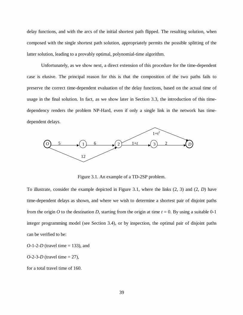
To illustrate, consider the example depicted in Figure 3.1, where the links (2, 3) and (2, D) have

time-dependent delays as shown, and where we wish to determine a shortest pair of disjoint paths

from the origin O to the destination D, starting from the origin at time t = 0. By using a suitable 0-1

integer programming model (see Section 3.4), or by inspection, the optimal pair of disjoint paths

can be verified to be:

O-1-2-D (travel time = 133), and

O-2-3-D (travel time = 27),

for a total travel time of 160.

5 6 1+t 2

12

1+t2

O 1 2 3 D

Figure 3.1. An example of a TD-2SP problem.

40

To try solving this problem by directly using the approach described in Suurballe and Tarjan

(1984), we first determine the shortest time-dependent path as O-1-2-3-D. This yields a travel time

of 25. Next we construct a residual graph G’ by reversing the links on the shortest path from node

O to node D, and by appropriately modifying arc costs or delay functions. However, in this

example, irrespective of how these arc delay functions are modified, by inspection, we can see that

the only path from O to D in G’ is O-2-D and this path is already disjoint with respect to the

shortest path in G. Hence, this yields the following pair of disjoint paths:

O-1-2-3-D (travel time = 25)

O-2-D (travel time = 157),

for a total travel time of 182 > 160.

Note again that this result is independent of any type of “modified” delay function that is

designed for the arcs in the residual network, although, in general, a suitable choice of such

modified delay functions could lead to results that are closer to optimality. Nonetheless, this

motivates the need for a more detailed study and a fresh approach for solving this TD-2SP problem.

3.3 Complexity Results

We begin by describing a new class of decision problems formulated by examining a

restriction of the more general TD-2SP problem. We show that even this restricted variant having a

single time-dependent arc is NP-Complete.

Decision variant of Problem RTD-2SP:

Suppose that we are given a graph having m nodes and n arcs along with a designated pair of nodes

O and D. Also, each arc has a constant integral travel time except for a single time-dependent arc

41

which has a travel time of 0 or 1, depending on the integral arrival time of entry at its tail node over

the interval [0, H], where H equals the sum of the other arc travel times. Then, for any integer K,

does there exist a pair of arc disjoint paths from O to D for which the total delay (travel time) is less

than or equal to K ?

Theorem 3.1. Problem RTD-2SP is NP-Complete.

Proof . The problem is clearly a member of NP since there exists a finite collection of pairs of arc-

disjoint paths between O and D, and given any certificate of such a pair of paths, it can be verified in

polynomial time whether or not its total travel time is less than or equal to K. Hence, it remains to

show that RTD-2SP is NP-Hard.

Toward this end, we perform a reduction from the NP-Complete partition problem. This

problem is given as follows (see Garey and Johnson (1979)):

Partition: Given n nonnegative integers a1, a2,..., an, where a Sii

n

= 21=

∑ , does there exist a partition

of these numbers into two sets such that the sum of each set equals S ?

Given any instance of this partition problem, we now derive an equivalent instance of Problem

RTD-2SP as follows:

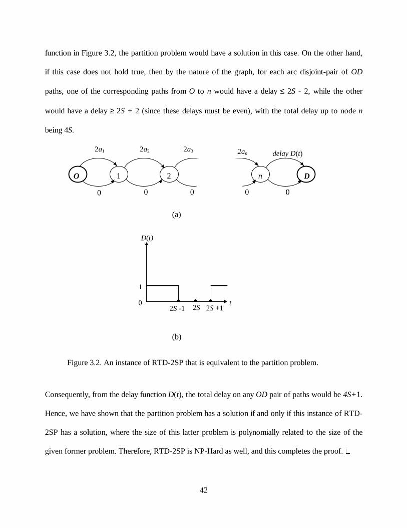
Construct a graph having (n+2) nodes, including O and D, and 2(n+1) arcs as shown in Figure 3.2,

where the delays on (n+1) of these arcs is zero, the delays on n other arcs are given by 2a1, 2a2,...,

2an, as indicated in Figure 3.2(a), and the delay on the remaining single arc from n to D is as

depicted in Figure 3.2(b). Furthermore, let K= 4S.

Now, let us consider two cases. First, suppose that there exists a pair of arc-disjoint paths

from O to n, both of which yield an arrival time at node n equal to 2S. Then, this would yield a pair

of arc-disjoint paths having a total delay of 4S. Moreover, by the nature of the graph and the delay

42

function in Figure 3.2, the partition problem would have a solution in this case. On the other hand,

if this case does not hold true, then by the nature of the graph, for each arc disjoint-pair of OD

paths, one of the corresponding paths from O to n would have a delay ≤ 2S - 2, while the other

would have a delay ≥ 2S + 2 (since these delays must be even), with the total delay up to node n

being 4S.

Consequently, from the delay function D(t), the total delay on any OD pair of paths would be 4S+1.

Hence, we have shown that the partition problem has a solution if and only if this instance of RTD-

2SP has a solution, where the size of this latter problem is polynomially related to the size of the

given former problem. Therefore, RTD-2SP is NP-Hard as well, and this completes the proof. �

O 1 2 n D

delay D(t) 2a1 2a2 2a3 2an

0 0 0 0 0

(a)

Figure 3.2. An instance of RTD-2SP that is equivalent to the partition problem.

D(t)

t 0

1

2S -1 2S +1 2S z z z

(b)

43

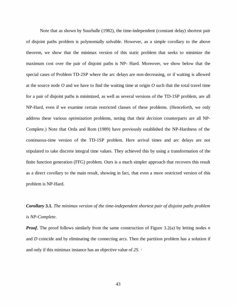
Note that as shown by Suurballe (1982), the time-independent (constant delay) shortest pair

of disjoint paths problem is polynomially solvable. However, as a simple corollary to the above

theorem, we show that the minimax version of this static problem that seeks to minimize the

maximum cost over the pair of disjoint paths is NP- Hard. Moreover, we show below that the

special cases of Problem TD-2SP where the arc delays are non-decreasing, or if waiting is allowed

at the source node O and we have to find the waiting time at origin O such that the total travel time

for a pair of disjoint paths is minimized, as well as several versions of the TD-1SP problem, are all

NP-Hard, even if we examine certain restricted classes of these problems. (Henceforth, we only

address these various optimization problems, noting that their decision counterparts are all NP-

Complete.) Note that Orda and Rom (1989) have previously established the NP-Hardness of the

continuous-time version of the TD-1SP problem. Here arrival times and arc delays are not

stipulated to take discrete integral time values. They achieved this by using a transformation of the

finite function generation (FFG) problem. Ours is a much simpler approach that recovers this result

as a direct corollary to the main result, showing in fact, that even a more restricted version of this

problem is NP-Hard.

Corollary 3.1. The minimax version of the time-independent shortest pair of disjoint paths problem

is NP-Complete.

Proof. The proof follows similarly from the same construction of Figure 3.2(a) by letting nodes n

and D coincide and by eliminating the connecting arcs. Then the partition problem has a solution if

and only if this minimax instance has an objective value of 2S. �

44

Corollary 3.2. Problem TD-2SP, with non-decreasing arc-delay costs, is NP-Hard, even if no more

than two arcs have time-dependent delays.

Proof. The proof follows similarly from the same construction of Figure 3.2 by replacing both the

arcs connecting n and D with time-dependent arcs, each having a delay D(t) as shown in Figure 3.3.

Hence, if both paths have a delay from node O to node n equal to 2S (implying that the partition

problem has a solution) then the objective value for this instance of TD-2SP would equal 4S.

Otherwise the cost would be equal to 4S+1. Hence the partition problem has a solution if and only if

this instance of TD-2SP has an objective value of 4S. This completes the proof. �

Corollary 3.3. Problem TD-2SP, where waiting is permitted at any node, is NP-Hard, even with no

more than two arcs having time-dependent delays.

Proof. By Corollary 2, since the non-decreasing delay version of TD-2SP with even 2 arcs having

time-dependent delays is NP-Hard, this means that any of the waiting time versions are NP-Hard for

this problem. �

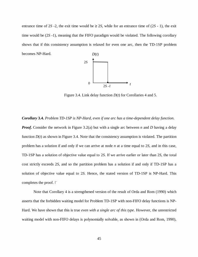
The TD-1SP problem with FIFO arc delays is polynomially solvable as shown by Kaufman

and Smith (1990). Note that the delay structure in Figure 3.2(b) satisfies the consistency

assumption. However, if the height of D(t) in Figure 3.2(b) for t < 2S - 1 is made ≥ 2, then for an

D(t)

t 0

1

2S

Figure 3.3. Link delay function D(t) for Corollary 2.

z

45

entrance time of 2S -2, the exit time would be ≥ 2S, while for an entrance time of (2S - 1), the exit

time would be (2S -1), meaning that the FIFO paradigm would be violated. The following corollary

shows that if this consistency assumption is relaxed for even one arc, then the TD-1SP problem

becomes NP-Hard.

Corollary 3.4. Problem TD-1SP is NP-Hard, even if one arc has a time-dependent delay function.

Proof. Consider the network in Figure 3.2(a) but with a single arc between n and D having a delay

function D(t) as shown in Figure 3.4. Note that the consistency assumption is violated. The partition

problem has a solution if and only if we can arrive at node n at a time equal to 2S, and in this case,

TD-1SP has a solution of objective value equal to 2S. If we arrive earlier or later than 2S, the total

cost strictly exceeds 2S, and so the partition problem has a solution if and only if TD-1SP has a

solution of objective value equal to 2S. Hence, the stated version of TD-1SP is NP-Hard. This

completes the proof. �

Note that Corollary 4 is a strengthened version of the result of Orda and Rom (1990) which

asserts that the forbidden waiting model for Problem TD-1SP with non-FIFO delay functions is NP-

Hard. We have shown that this is true even with a single arc of this type. However, the unrestricted

waiting model with non-FIFO delays is polynomially solvable, as shown in (Orda and Rom, 1990),

D(t)

t 0

2S

2S -1

Figure 3.4. Link delay function D(t) for Corollaries 4 and 5.

z

46

after modifying the delay functions to essentially equivalently yield a FIFO delay structure. This is

done by building in delays dependent on arrival times.

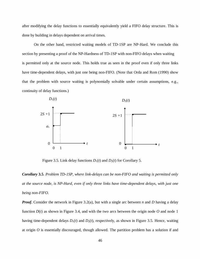
On the other hand, restricted waiting models of TD-1SP are NP-Hard. We conclude this

section by presenting a proof of the NP-Hardness of TD-1SP with non-FIFO delays when waiting

is permitted only at the source node. This holds true as seen in the proof even if only three links

have time-dependent delays, with just one being non-FIFO. (Note that Orda and Rom (1990) show

that the problem with source waiting is polynomially solvable under certain assumptions, e.g.,

continuity of delay functions.)

Corollary 3.5. Problem TD-1SP, where link-delays can be non-FIFO and waiting is permitted only

at the source node, is NP-Hard, even if only three links have time-dependent delays, with just one

being non-FIFO.

Proof. Consider the network in Figure 3.2(a), but with a single arc between n and D having a delay

function D(t) as shown in Figure 3.4, and with the two arcs between the origin node O and node 1

having time-dependent delays D1(t) and D2(t), respectively, as shown in Figure 3.5. Hence, waiting

at origin O is essentially discouraged, though allowed. The partition problem has a solution if and

Figure 3.5. Link delay functions D1(t) and D2(t) for Corollary 5.

D1(t)

t 0

a1

0 1

z

z

2S +1

D2(t)

t 0 0 1

z

z

2S +1

47

only if we can arrive at node n at a time equal to 2S (with zero waiting time at origin O), and in this

case, TD-1SP has a solution with an objective value equal to 2S. If we arrive at node n at a time

earlier or later than 2S, the total cost strictly exceeds 2S, and so, the partition problem has a

solution if and only if TD-1SP has a solution having an objective value equal to 2S. Hence, the

stated version of TD-1SP is NP-Hard. This completes the proof. �

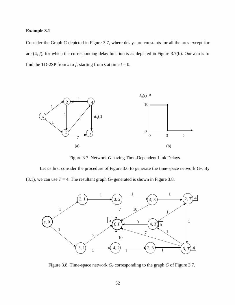
3.4 A 0-1 Linear Programming Model for Problem TD-2SP

Consider a digraph G’(N’, A’), where N’ and A’ are the sets of nodes and arcs of G’,

respectively. Furthermore, suppose that we have a designated pair of origin (start) and destination

(final) nodes s and f, respectively. Let the start time at the origin node s be 0, and suppose that we

are interested in finding a TD-2SP from s to f, where the travel delays are defined on a discrete set

of times S = { 0, δ, 2δ,....., Mδ} → {0, δ, 2δ, ..., M’δ}, for some integer M’ and for some suitably

large value of M. (Note that Mδ merely puts a practical limit on time beyond which the

characterization of the delay function is not of interest.) Hence, the nodes of G’ are visited along

any path at the discrete points in time specified by S. Observe that this delay structure could be

viewed as a discretized approximation to some general specified set of arc delay functions.

Without loss of generality, assume that the network has been preprocessed so that FS(f) =

∅ and RS(s) = ∅, where FS(⋅) and RS(⋅) respectively denote the forward and reverse stars of any

node (⋅). Additionally, suppose that we find all the nodes that are reachable from s by successively

scanning FS(⋅), starting at s, and that we find all nodes that can reach f by successively scanning

RS(⋅), starting at f. Let N ⊆ N’ be the set of nodes in the intersection of these two resulting node

sets, and let G(N, A) be the subgraph of G’ induced by this node set N. Clearly, we only need to

focus on this subgraph G in order to solve the stated TD-2SP problem from s to f.

48

Now, define

UB = some upper bound on the length (delay) of any acceptable path in the solution to TD-

2SP,

NOW = {( s, 0)}

NEXT = ∅

(SE ≡ NOW ∪ NEXT)

λ(s,0) = 0NOW = ∅ ?

NEXT = ∅ ?

STOP

Pick (p, t)

∈ NOW

Put

NOW = NEXT

NEXT = ∅

Scan FS(p) in G. For each arc (p, q) ∈ A

corresponding to q ∈ FS(p), DO:

(a) Compute tq = λ(p,t) + dpq[ λ(p,t) ]. If tq > T,

or if FS (q) = ∅, go to (c).

Else, proceed to (b).

(b) i. Create a node (q, tq) for GT if it

doesn’t already exist. Put λ ( ,q tq qt) = .

ii. Create an arc (p, t) → (q, tq) having a

delay equal to dpq[t].

iii . If (q, tq) ∉ SE and it has been newly

created at this visit to (b)i., put it in NEXT.

Return to the top of this loop.

(c) i. Create a node (q, T) for GT, if it

doesn’t already exist, and in this case, let

λ(q,T) = ∞ temporarily.

ii . Create an arc (p, t) → (q, T) having a

delay = dpq[t], if it doesn’t already exist.

iii . If tq < λ(q,T), then revise the label λ(q,T) to

tq, and then, if (q, T) ∉ SE and FS(q) ≠ ∅,

put (q, T) in NEXT.

Return to the top of this loop.

Remove (p, t)

from NOW

Y

Y

N

N

Comment: λ(p,t) ≡ t for t < T, and

so, λ(p,t) is required only for t = T.

Figure 3.6. Generation of GT (NT, AT) and the solution of TD-1SP on G.

49

BP = delay function breakpoint such that dij(ti) is a constant for ti ≥ BP, for each (i, j) ∈ A,

and let

T = minimum {UB, BP}. (3.1)

We will now use this parameter T to govern the degree with which each node in G is replicated in a

time-space representation of the given network. Note that for static problems, we would have T = 0

by virtue of the second term in the minimand in (3.1), and hence, no replicates would be necessary.

Otherwise, either an upper bound on the path length, or the time beyond which the delay step

function is flat for all arcs will influence the extent of replications.

It is well known that there exists a time-space static equivalent network representation for

this problem (Kaufman and Smith, 1990). In this representation, each node is replicated as {i, t} ∀t

∈ S. Furthermore, for each (i, j) ∈ A, we construct an arc {(i, t), (j, t+ dij (t))} having a fixed delay

of dij(t),∀t ∈ S such that t+ dij (t) ≤ Mδ, where note that t + dij (t) then also belongs to S by our

assumption. Hence, each node and arc gets replicated (up to) |S| times.

We will now describe a procedure that dynamically generates a reduced-size time-space

network using a minimal number of time-based node replications, while simultaneously finding the

TD-1SP from s to f. This is done within the framework of a dynamic programming routine for

finding the shortest time-dependent path from s to all the nodes in G, and therefore also to f,

implemented using an extension of the partitioned shortest path (PSP) algorithm for the static case

due to Glover, et al. (1985). Figure 3.6 describes the proposed network generation procedure.

Here, time-expanded replicates (p, t) of each node p ∈ N are automatically created only for specific,

necessary values of t, based on possible visitation times. Let GT (NT, AT) denote the time-space

network that is generated by this procedure. Note that we obtain

50

minimumt

λ(p, t) = delay for the TD-1SP from node s to node p, ∀ p ∈ N (3.2)

where the minimum in (3.2) is taken over all the nodes (p, t) created in this process. Moreover, the

actual shortest path that yields the delay (3.2) can be traced by maintaining appropriate predecessor

labels while revising the λ-labels, as described in Glover, et al. (1985).

Remark 3.1: Consider a time-independent SP problem having nonnegative delays. Then T = 0 in

(3.1), and the procedure of Figure 3.6 would create GT ≡ G, and in essence, this procedure is

precisely the polynomial-time PSP algorithm of Glover, et al. (1985), having a complexity of

O(|N||A|). In fact, if we have mixed-sign costs (but no negative cost circuits), then by artificially

letting T be any number that is less than the sum of the negative costs in the procedure of Figure

3.6, this would also solve the underlying 1-SP problem with the same polynomial-time complexity.

Remark 3.2: Likewise, for the time-dependent problem having FIFO delay functions, by taking T ≡

0 (rather than using (3.1)), this algorithm will determine the TD-1SP from s to all the nodes in G in

polynomial time of complexity O(|N||A|).

Remark 3.3: Consider the time-dependent problem having arc delays described by step-functions as

described above. Then for each node p N∈ , (3.2) gives the TD-1SP from node s to node p

(assuming that the upper bound in (3.1) exceeds (≥) this path length). Moreover, this algorithm

generates a time-space network GT in which for each path in G having some time-dependent length,

there corresponds a representative static path in GT that has the same length (again assuming that

the upper bound in (3.1) exceeds (≥) this path length ).

Now, tentatively suppose that we apply the SPDP algorithm in Suurballe and Tarjan (1984)

to this expanded network GT, considering a starting time of t0 = 0 for node s. This algorithm first

requires the determination of the ordinary SP tree T’ on GT. Assume that this process yields a

51

corresponding simple time-dependent shortest path from s to f on the original graph G. If we now

continue to follow the procedure of Suurballe and Tarjan (1984) for solving the SPDP problem on

GT, we might arrive at two arc-disjoint paths on GT that include copies of some particular arc in G.

Translating this solution from GT to G, since this would correspond to using this same arc in G on

both these paths, the solution would not yield an arc-disjoint pair of paths in this case. Hence, we

need to add side-constraints that prevent any arc in G from being used in more than one path in the

final solution in GT. This feature requires us to use a 0-1 model, thereby injecting nonconvexity into

the problem.

Before presenting our model, note that we would indeed impose a non-implied restriction if

we enforced that each arc be used at most once in the overall solution. In particular, such a

constraint would preclude arcs from being used more than once for even a single path, i.e., it would

enforce paths to be arc-simple. For FIFO delay situations, we would not need to consider non-

simple paths and so such a model would yield a valid representation for the underlying problem.

However, for non-FIFO delays where TDSPs can include loops, a model of this type would prohibit

such paths. In the sequel, we consider both the above types of models that permit non-simple as

well as enforce arc-simple paths, as well as other models that require relaxed versions of

disjointedness. But before developing these models, let us present an example to illustrate the

procedure of Figure 3.6 and how non-FIFO delays can lead to looped paths. We shall then use this

example to illustrate the results of our different proposed models.

52

Example 3.1

Consider the Graph G depicted in Figure 3.7, where delays are constants for all the arcs except for

arc (4, f), for which the corresponding delay function is as depicted in Figure 3.7(b). Our aim is to

find the TD-2SP from s to f, starting from s at time t = 0.

Let us first consider the procedure of Figure 3.6 to generate the time-space network GT. By

(3.1), we can use T = 4. The resultant graph GT generated is shown in Figure 3.8.

Figure 3.8. Time-space network GT corresponding to the graph G of Figure 3.7.

1 1

s, 0

2, 1

3, 1

3, 2

4, 2

1

1

1

7

4, 3

2, 3 3, T

2, T

4, T f, T

7 7

0

1

1

1

1

1

1

10

10

4

4

5 5

(b)

0 t

d4f(t)

0

10 z

3

(a)

s

2

3

4

f

1

1

1

1 1

7

d4f(t)

Figure 3.7. Network G having Time-Dependent Link Delays.

53

Note that by the comment given in Figure 3.6, the labels λ(p, t) are equal to t ∀ nodes (p, t)

having t < T, while for the nodes (p, T), these labels are shown against the corresponding nodes.

Also, by (3.2), the TD-1SP to nodes 2, 3, 4 and f from s are respectively of lengths 1, 1, 2 and 5. In

particular, observe that the TD-1SP to node f is given by {(s, 0)-(3, 1)-(4, 2)-(2, 3)-(3, T)-(4, T)-(f,

T)}. This corresponds to the non-simple path {s-3-4-2-3-4-f} in G.

Consider now the TD-2SP problem. Permitting non-simple paths, the shortest pair of

disjoint paths are given by {s-2-3-4-2-3-4-f} and {s-3-f}, having a total length of 14. However, if

we restrict the paths to be simple, the optimal pair of disjoint paths become {s-2-3-4-f} and {s-3-f},

or {s-2-3-f} and {s-3-4-f}. Both these pairs of paths have a total length of 21 > 14.

We now present models to determine the time-dependent shortest pair of disjoint paths

under the various restrictions discussed above. First, let us consider the case where non-simple

paths are allowed. Because of the permissibility for arcs to repeat for any given path, but not

between paths, we need to carry the two path flows separately in the model. These path flows are

respectively identified by variables x and y as follows. Given GT as generated by Figure 3.6, let

xij i j GT = if arc ( ) of is in path #1

0 otherwise,

1 ,

(3.3a)

and

yij i j G T = if arc ( ) of is in path #2

0 otherwise. 1 ,

(3.3b)

Furthermore, for each arc “k” in G, k = 1, 2,..., K, say, define

Sk = { Arcs of GT that represent copies of arc k in G }, for k = 1, 2,..., K. (3.4)

The following 0-1 model TD-2SP(NS) then represents the problem of finding non-simple (NS)

shortest pair of disjoint paths. Here, FST(⋅) and RST(⋅) respectively denote the forward and reverse

54

stars of nodes (⋅) in GT. Note that constraints (3.5b) and (3.5c) represent the shortest path network

flow constraints for each of the individual paths, while the side-constraints (3.5d) restrict these

paths to be disjoint. Because of these side-constraints, extreme points of (3.5b)-(3.5e) are not

necessarily binary valued, and hence, (3.5f) is not superfluous.

TD-2SP(NS):

)(3.5a )( Minimize),(

∑∑∈

+TAji

ijijij yxd

subject to:

)b5.3(

otherwise 0

),(for 1

)0,(for 1

)()(∑∑

∈∈

≡−

≡

=−iRSj

jiiFSj

ij

TT

Tfi

si

xx

)c5.3(

otherwise 0

),(for 1

)0,(for 1

)()(∑∑

∈∈

≡−

≡

=−iRSj

jiiFSj

ij

TT

Tfi

si

yy

)d5.3( .,...,2,1 and,),( ,),( 1 KkSqpSjiyx kkpqij =∈∈∀≤+

)e5.3( ),( 10 and 10 Tijij Ajiyx ∈∀≤≤≤≤

x, y binary. (3.5f)

Remark 3.4: Note that there are | |k

kS=

∑1

2K

constraints in (3.5d). Also, the upper bounds in (3.5e) are

implied by (3.5d) and the nonnegativity restrictions in (3.5e), but are explicitly stated here only for

clarity. The LP relaxation of this problem is defined by (3.5a) - (3.5e).

55

Remark 3.5: If multiple start times need to be considered for the TD-2SP problem, then our

procedure would need to be repeated for each given possible start time at node s. On the other

hand, note that for the TD-1SP problem, if the TDSP is required from all nodes to node f for all

possible start times in a given set, then the multi-state labeling procedure of Mahmassani, et al.

(1994) can be used, based on a backward recursion. Note that in our case of Figure 3.6, if some

specified start-times at node s were given, say in a set ST ⊆ {0, δ, 2δ,...}, then we could create a

node (s, t) for each t ∈ ST initially and place this in NOW, and then we could follow the same

scheme to find the TD-1SP from s to f for each start time node, except that we would now carry

multiple labels corresponding to each start time.

Alternate Types of Side-Constraints

In many practical cases, the user may be interested in dealing with only arc-simple paths,

even if they are non-optimal with respect to TD-2SP(NS) as illustrated previously in Example 3.1.

Hence, it would be desirable to reformulate the side-constraints (3.5d) such that the solution yields

optimal arc-simple paths. This might be more practical, especially when combined with different

starting times in order to prescribe waiting-induced departure times at the origin node. To model

this case, we only need to define one set of binary flow variables Xij, where

)6.3( otherwise. 0

patheither on used is of ),( arc if 1

=T

ij

GjiX

Observe that now, the X-variables must represent a flow of two units from s to f, one along each

identified path, where the corresponding two paths jointly use any link of G at most once. This can

be modeled as follows.

56

TD-2SP(S):

)(3.7a Minimize),(

∑∑∈ TAji

ijij Xd

subject to:

)b7.3(

otherwise 0

),(for 2

)0,(for 2

)()(∑∑

∈∈

=−

=

=−iRSj

jiiFSj

ij

TT

Tfi

si

XX

)d7.3( binary. ,),( 10

)c7.3( ,...,2,1 1),(

XAjiX

KkX

Tij

Sjiij

k

∈∀≤≤

=∀≤∑∈

Let us now simplify the form of (3.7) for the special case in which the shortest path in GT from s to f

corresponds to a shortest simple path in G for problem TD-1SP. Hence, this path in GT satisfies the

side-constraints (3.7c). Let X’ij =1 if (i, j) ∈ AT belongs to this shortest path and X’ij = 0 otherwise.

Also, using the shortest path labels λi ∀ i ∈ NT as obtained in Figure 3.6, let us denote the reduced

costs d’ij as:

d’ij = dij + λi - λj ∀ (i, j) ∈ AT. (3.8)

Furthermore, define

P = {( i, j)∈AT : X’ij = 1}. (3.9)

Now, let us use the transformation

Yij = Xij ∀ (i, j) ∈ AT - P, Yji = 1 - Xij ∀ (i, j) ∈ P. (3.10)

Note that arc (i, j) ∈ P is flipped in the transformed problem. Then, (3.7) gets transformed to the

following problem. (Note that dij can be equivalently replaced by d’ij in (3.7), and that d’ij = 0 if (i, j)

57

∈ P. Also, here, FS and RS refer to the forward and reverse star functions on the graph that is

transformed under (3.10).)

TD-2SP(S)’:

)(3.11a Minimize),(

'∑∑ji

ijij Yd

subject to:

)b11.3(

otherwise 0

),(for 1

)0,(for 1

)()(∑∑

∈∈

≡−

≡

=−iRSj

jiiFSj

ij

TT

Tfi

si

YY

)e11.3( binary. ,),( 10

)d11.3( )},{( where,

)c11.3( 1

},{),(

),(

YjiY

qpSPSPkYY

SPkY

ij

kkqpqpSji

ij

kSji

ij

k

k

∀≤≤

=∩∅≠∩∋∀≤

∅=∩∋∀≤

∑

∑

−∈

∈

Note that problem (3.11) effectively seeks a shortest path from s to f subject to the side-constraints

(3.11c) and (3.11d). Also, note that |P∩Sk|≤ 1 ∀ k = 1, 2,..., K. Due to its modified structure, in the

presence of alternative optimal solutions to the LP relaxation, the fractionality of variables resulting

at optimality for the relaxation of (3.11), as opposed to that obtained for (3.7), might differ. Hence,

whenever the shortest path in GT from s to f yields a simple path in G, we can equivalently use the

revised model (3.11). Some computational experience comparing the use of these alternative

models is presented in the following section.

Example 3.2

Consider the network G of Figure 3.7 and its corresponding time-space network GT shown

in Figure 3.8. Let us now use models (3.5) and (3.7) to find the non-simple and the arc-simple TD-

58

2SP from s to f respectively, starting from s at time t = 0. We can formulate the side-constraints for

model (3.5) by comparing Figures (3.7) and (3.8). For example, the arcs ((2, 1), (3, 2)), ((2, 3), (3,

T)) and ((2, T), (3, T)) in GT are three copies of the same arc (2, 3) in G. While any or all of these

three arcs can be used on a single path from s to f, using any copy in one path disallows the use of

these arcs for the other path. For the same example, the side-constraints for model (3.7) would

differ from those for model (3.5) by stipulating that only one of these three copies can be used even

for a single path. The LP relaxation of model (3.5) was solved using the CPLEX-MIP package and

an optimal objective value of 14.0 was obtained with fractional flows on the arcs. The optimal IP

solution was obtained after enumerating one branch-and-bound node, producing a solution having

an optimal total delay cost of 14, and yielding the optimal pair of non-simple disjoint paths

previously discussed in Example 3.1. The LP relaxation for model (3.7) resulted in an all-integer

solution with an optimal delay cost of 21, yielding the pair of simple disjoint paths {s-3-f} and {s-2-

3-4-f}. Another pair of disjoint paths, {s-2-3-f} and {s-3-4-f}, can also be found, with the same

total delay cost of 21. In this case, problem TD-2SP(S) has multiple optimal solutions. Model

(3.11) is not applicable here, since the TD-1SP solution yields a non-simple path.

Remark 6: The nature of the foregoing side-constraints facilitates easy manipulation, so that they

can be imposed (only) for certain user-specified arcs, depending on the type of application and

scenario. For example, in a transportation network, if a particular link happens to be a freeway

having a large capacity, it might not be practically useful to prevent the traffic on the prescribed pair

of paths from being disjoint with respect to this arc. Alternatively, we might be interested in simply

preventing the flows on the prescribed two paths from overlapping in time while using certain arcs,

while permitting both the paths to use these arcs otherwise. For example, links that are potential

59

candidates for bottlenecks during peak hour traffic may be subjected to these side-constraints. In the

context of model (3.5), for either of these scenarios, we would then accordingly relax those

constraints in (3.5d) that no longer represent imposed restrictions. Note that if in addition we were

required to generate simple paths, then because we need to maintain the separate identities of the

two path flows under such scenarios, we would continue to use model (3.5) instead of using model

(3.7). However, we would now impose additional constraints of the type (3.7c) for each of the x

and y variables, or for the joint set of x and y variables, whichever is valid, depending on the

context.

To illustrate, consider the example of Figures 3.7 and 3.8, and suppose that we relax the

disjointedness requirement for the arc (3, f) in G, requiring only arc-simple paths to be considered.

Then, in model (3.5), instead of (3.5d), we would impose

( ( , ),( , )

x y k fij iji j Sk

+∑ ≤ ∀ ≠∈

) 1 3

x y k fiji j S

iji j Sk k( , ) ( , )

).

1 and 1 for (3, ∈ ∈

∑ ∑≤ ≤ ≡

Running this model, we obtained the pair of partially disjoint simple paths {s-3-f} and {s-2-3-f},

having a total delay cost of 17. Note that arc (3, f) is present in both paths.

3.5 Computational Results

The proposed models were tested for two kinds of networks:

i. Random networks of different densities and having random delays.

ii. The network instances that correspond to the partition problem as depicted in Figure 3.2.

60

Random Networks

Random digraphs having m nodes and density ρ were generated using the procedure given

in Skiscim and Golden (1989) as follows. Let the number of arcs, n, be given by ρm(m-1). The

values of the density ρ range from 0 to 1. First we generate random (static) delays for the complete

graph having m(m-1) arcs and we find the shortest path tree rooted at a given origin. We then add

the remaining {ρm(m-1)-(m-1)} arcs to this tree graph based on whether a random number

generated for each of the remaining arcs in the complete graph exceeds a given threshold value. To

model delays, piecewise-continuous non-negative polynomial functions of time were used, having

random coefficients and degrees, and these were then discretized into step functions using δ = 1.

The delay functions generated can admit non-simple paths, since the consistency assumption was

not enforced.

The problems were run using the CPLEX-MIP package on a UNIX - Sun SPARC 1000

computer for each of the models (3.5), (3.7), and (3.11), where applicable. The computational time

and the number of branch-and-bound tree nodes enumerated for each model are given in Table 3.1.

Here, m, n, and M are respectively the number of nodes and arcs in G, and the number of time-

periods for the delay function step breakpoints. The next two columns give the linear programming

(LP) effort (CPU seconds) required to solve the relaxation and its objective value, and the last three

columns give the additional time required to solve the integer program (IP), the number of branch-

and-bound nodes generated in the process, and the optimal IP objective value. The objective values

reported for model (3.11) include the constants resulting from the transformation of model (3.7).

61

Table 3.1

(a) Model (3.5)

Nodes(m)

Arcs(n)

Timeperiods (M)

Time forLP (sec)

LPOpt

Time forIP(sec)

IPnodes

IPOpt

20 40 20 0.44 9 0.0 0 950 75 20 0.80 8.0 1.26 4 1740 100 30 21.01 37.0 161.03 25 62100 500 10 8.89 2.0 0.0 0 2200 500 50 23.56 879.0 30.28 2 1394

(b) Model (3.7)

Nodes(m)

Arcs(n)

Timeperiods (M)

Time forLP(sec)

LPOpt

Time forIP(sec)

IPnodes

IPOpt

20 40 20 0.06 9.0 0.0 0 950 75 20 0.10 17.0 0.0 0 1740 100 30 0.71 62.0 0.0 0 62100 500 10 0.88 2.0 0.0 0 2200 500 50 1.71 1394 0.0 0 1394

(c) Model (3.11)

Nodes(m)

Arcs(n)

Timeperiods (M)

Time forLP(sec)

LPOpt

Time forIP(sec)

IPnodes

IPOpt

20 40 20 0.05 9.0 0.0 0 950 75 20 0.10 17.0 0.0 0 1740 100 30 0.54 62.0 0.0 0 62100 500 10 0.84 2.0 0.0 0 2200 500 50 1.35 1394 0.0 0 1394

Table 3.1 highlights the tightness of the continuous relaxation to TD-2SP(S) (and TD-2SP(S)’), in

that for all the cases reported in Table 3.1, no branching was required and the relaxed LP produced

optimal 0-1 flow values. We can also see that in each test case, the optimal paths were arc-simple,

since the optimal IP values for models (3.5) and (3.7) (and (3.11)) coincide. However, by using

random delays within a highly restricted range [0, 4], one test case was found that gave both,

62

fractional flows and non-simple optimal paths. The corresponding results for this case are shown in

Table 3.2.

Table 3.2

a. Model (3.5)

Nodes(m)

Arcs(n)

Timeperiods (M)

Time forLP(sec)

LPOpt

Time forIP(sec)

IPnodes

IPOpt

100 200 5 0.99 2.0 5.00 14 3

b. Model (3.7)

Nodes(m)

Arcs(n)

Timeperiods (M)

Time forLP(sec)

LPOpt

Time forIP(sec)

IPnodes

IPOpt

100 200 5 0.23 2.5 0.10 1 3

c. Model (3.11)

Nodes(m)

Arcs(n)

Timeperiods (M)

Time forLP(sec)

LPOpt

Time forIP(sec)

IPnodes

IPOpt

100 200 5 0.20 2.0 0.13 2 3

While the optimal IP values obtained via models (3.5) and (3.7) are the same, model (3.5) actually

produced a non-simple pair of disjoint paths. This implies that model (3.5) has multiple optimal

solutions, since any optimal solution to model (3.7) is feasible to model (3.5).

Network Instances of the Partition Problem

The integers {ai, i = 1, ..., n} were randomly generated. Let a Sii

n=

=∑ 2

1. The dummy arcs having

zero delays were split into two serial arcs, each of zero delay. Hence, for n integers, the number of

arcs equals 3n+3 and the number of nodes equals 2n+3. The number of time periods, M, was set

equal to 4S+1.

63

Table 3.3 presents the results obtained. Note that the network for this problem does not

include the possibility of non-simple paths. However, ignoring this fact in formulating model (3.5)

results in a considerably weaker LP relaxation than that obtained for models (3.7) and (3.11), hence

requiring a significantly greater solution effort for this model. Observe that for the models (3.7) and

(3.11), in each of the test cases reported in Table 3.3, the optimal objective function value of the LP

relaxation was equal to the final IP optimal value. Hence, the enumeration required was to

essentially find an alternative optimal LP solution that happened to binary. A comparison of the

results in Table 3.3(b) and 3.3(c) indicates the relative advantage of formulating the problem as one

of finding a shortest path in the transformed network represented by model (3.11) in contrast with

the direct use of model (3.7). Due to its structure, model (3.11) has a greater propensity toward

producing discrete solutions via its LP relaxation, when such solutions exist, and is therefore

recommended for use over model (3.7) whenever applicable.

Table 3.3

a. Model (3.5)

n 4S Time for LP (sec) LP Opt Time for IP (sec) Nodes (IP) IP Opt5 28 0.49 10 3.24 31 2910 30 1.13 4 38.63 190 3110 74 6.05 10 915.04 766 7510 120 14.78 16 2157.11 483 12010 252 64.13 32 2141.36 501 25215 92 15.02 10 34048.16 8516 92

64

b. Model (3.7)

n 4S Time for LP (sec) LP Opt Time for IP (sec) Nodes (IP) IP Opt5 28 0.06 29 0.03 2 2910 30 0.11 31 0.02 0 3110 74 0.35 75 0.88 3 7510 120 0.35 120 30.78 22 12010 252 0.60 252 62.54 5 25215 92 1.01 92 161.29 32 9220 340 13.76 340 5579.5 12 340

c. Model (3.11)

n 4S Time for LP (sec) LP Opt Time for IP (sec) Nodes (IP) IP Opt5 28 0.03 29 0.02 0 2910 30 0.12 31 0.16 7 3110 74 0.35 75 0.24 2 7510 120 0.39 120 1.61 8 12010 252 0.66 252 1.10 3 25215 92 1.00 92 21.62 27 9220 340 18.64 340 468.32 5 340

3.6 Summary, Conclusions and Future Research

In this study, we have examined the time-dependent shortest pair of disjoint paths problem

(TD-2SP). This problem, including its selectively disjoint path variants, finds applications in

dynamic traffic routing and assignment procedures in the context of Intelligent Transportation

Systems (ITS). A computational complexity analysis was performed to exhibit that this

(optimization) problem as well as several of its variants are all NP-Hard, even under mild departures

from the corresponding time-dependent, polynomially solvable class of problems. Subsequently, a

0-1 linear programming model was developed to solve the TD-2SP problem. This model can

accommodate various degrees of disjointedness of the paths, and some simplified representations

can be obtained when the optimal pair of paths are required to be arc-simple. Computational tests

using randomly generated networks, and network instances of the partition problem reveal the

65

efficacy of the proposed models. In particular, the computational requirements for the specialized

models formulated to determine a time-dependent shortest pair of arc-simple disjoint paths is

considerably less than that required by the general TD-2SP model in this case. Hence, these

specialized models are recommended for use whenever applicable.

Future research possibilities include the study of various applications of TD-2SP, and its

minimax variant, in transportation and communication network flow problems. The relative

advantages of using TD-2SP for the minimum-risk routing of hazmat carriers and the routing of

multiple emergency-response vehicles in comparison with currently used routing methods can be

investigated. The efficacy of prescribing selectively disjoint paths as a routing tool in a dynamic

traffic assignment procedure is another interesting subject of future study.