Chapter 3 Two major topics of this chapter: Ch t 3Chapter...

1

Ch t 3Chapter 3

Discrete-Time Fourier Transform (DTFT)Fourier Transform (DTFT)

Chapter 3

Two major topics of this chapter: Discrete-Time Fourier Transform

Discrete-Time Fourier Transform(DTFT) DTFT Theorems Spectrum Analysis

Discrete-Time System in Frequency Domain

2

Domain Frequency Response of an LTI Discrete-Time System Phase and Group Delay The Unwrapped Function

Ch t 3AChapter 3A

Discrete-Time Fourier TransformFourier Transform

Part A: DTFT

1. 1. The ContinuousThe Continuous--Time Fourier TransformTime Fourier Transform1 11 1 D fi itiD fi iti 1 21 2 E D it S tE D it S t1.11.1 Definition Definition 1.21.2 Energy Density SpectrumEnergy Density Spectrum1.31.3 BandBand--limited Continuouslimited Continuous--Time SignalsTime Signals

2. The Discrete2. The Discrete--Time Fourier TransformTime Fourier Transform2.12.1 Definition Definition 2.2 2.2 Basic PropertiesBasic Properties2.32.3 Symmetry RelationsSymmetry Relations 2.42.4 Convergence Condition Convergence Condition

3 DTFT Computation Using MATLAB3 DTFT Computation Using MATLAB

4

3. DTFT Computation Using MATLAB3. DTFT Computation Using MATLAB4. DTFT4. DTFT TheoremsTheorems5. Energy Density Spectrum5. Energy Density Spectrum6. Band6. Band--limited Discretelimited Discrete--Time SignalsTime Signals

2

1.1 Definition of CTFT

DefinitionDefinitionDefinitionDefinition

The CTFT of a continuous-time signal xa(t) is given by

( ) ( ) j ta aX j x t e dt

analysis equation

5

Often referred to as the Fourier SpectrumFourier Spectrum or simply the SpectrumSpectrum of the continuous-time signal


The inverse CTFT of a Fourier Transform The inverse CTFT of a Fourier Transform Xa(jΩ) is given by

Often referred to as the Fourier integralFourier integral

1( ) ( )2

j ta ax t X j e d

synthesis equation

6

A CTFT pair will be denoted as CTFT( ) ( )a ax t X j


Ω is real and denotes the continuous-time Ω is real and denotes the continuous time angular frequency variable in rad/s

In general, the CTFT is a continuous complex function of Ω in the range −∞<Ω< ∞

It can be expressed in the polar formpolar form as

7

where( )( ) ( ) aj

a aX j X j e

( ) arg{ ( )}a aX j


Th tit |X (jΩ)| i ll d th it dit d The quantity |Xa(jΩ)| is called the magnitude magnitude spectrumspectrum and the quantity θa(Ω) is called the phase spectrumphase spectrum；both spectrums are realfunctions of Ω

In general, the CTFT Xa(jΩ) exists if xa(t)

8

In general, the CTFT Xa(jΩ) exists if xa(t)satisfies the DirichletDirichlet Conditions Conditions given on the next slide：

3


Di i hl tDi i hl t C ditiC ditiDirichletDirichlet ConditionsConditions(a) The signal xa(t) has a finite number of discontinuities and a finite number of maxima and minima in any finite interval

(b) Th i l i b l t l i t bl i

9

(b) The signal is absolutely integrable, i.e.

( )ax t dt


If the DirichletDirichlet ConditionsConditions are satisfied then If the DirichletDirichlet ConditionsConditions are satisfied, then

converges to xa(t) at values of t except at values of t where xa(t) has discontinuities

1 ( )2

j taX j e d

10

a( ) It can be shown that if xa(t) is absolutely absolutely

integrableintegrable, then |Xa(jΩ)| <∞ proving the existence of the CTFT


ExampleExampleExampleExample Find the CTFT of the following signal

Sol tion:

0,00,

t

a

tex t

t

11

Solution:

( )00

1 1( ) t j t j taX j e e dt e

j j


2

0t te

-4 -2 0 2 40

0.5

1

1.5

, in radians

Mag

nitu

de

1.50.6

0.8

1

e

0,

0.500,a

tex t

t

12

-4 -2 0 2 4-1.5

-1

-0.5

0

0.5

1

, in radians

Pha

se,in

radi

ans

-5 0 5 10-0.2

0

0.2

0.4

t

Am

plitu

d

4


ExampleExampleExampleExample Find the CTFT of the following signal

( ) ( )t t t

( ) ( ) 1j tax t t j t e dt

13

0( ) ( )ax t t t

otjtjoa edtettjX

)()(

1.2 Energy Density Spectrum

The total energy of a finite energy The total energy x of a finite energy continuous-time complex signal xa(t) is given by

The above expression can be rewritten as

2 *( ) ( ) ( )x a a ax t dt x t x t dt

14

The above expression can be rewritten as

*1( ) ( )2

j tx a ax t X j e d dt


I t h i th d f th i t ti Interchanging the order of the integrations, we get

*

*

1 ( ) ( )21 ( ) ( )

jx

ta a

X

X j x t e dt d

j X j d

15

21 ( )

( )2

2

( )a a

a

X j X j

j

d

X d


Hence

The above relation is more commonly known

2 21( ) ( )2a ax t dt X j d

16

yas the Parseval’sParseval’s relationrelation for finite energy continuous-time signals

5


The quantity |Xa(jΩ)|2 is called the energy energy e qu y | a(j )| s c ed e e e gye e gydensity spectrumdensity spectrum of xa(t) and usually denoted as

The energy over a specified range of

2( ) ( )xx aS X j

17

gy p gfrequencies Ωa≤Ω≤Ωb can be computed using

,1 ( )

2b

ax r xxS d

1.3 Band-limited Continuous-Time Signals

A fullfull--bandband, finite-energy, continuous-time signal has a spectrum occupying the whole whole frequency rangefrequency range −∞<Ω< ∞

A bandband--limitedlimited continuous-time signal has a spectrum that is limited to a portion of thea portion of the

18

spectrum that is limited to a portion of the a portion of the frequency rangefrequency range −∞<Ω< ∞


An ideal bandideal band limitedlimited signal has a spectrum An ideal bandideal band--limitedlimited signal has a spectrum that is zero outside a finite frequency range Ωa≤|Ω|≤Ωb , that is

0, 0( )

0,a

ab

X j

19

However, an ideal band-limited signal cannot be generated in practice (WhyWhy?)?)

0, b


B dB d li it d i lli it d i l l ifi d di BandBand--limited signals limited signals are classified according to the frequency range where most of the most of the signal’s is concentratedsignal’s is concentrated

A lowpasslowpass, continuous-time signal has a spectrum occupying the frequency range

20

spectrum occupying the frequency range |Ω|≤Ωp<∞ where Ωp is called the bandwidthbandwidth of the signal

6


A highpasshighpass, continuous-time signal has a spectrum occupying the frequency range 0<Ωp ≤ |Ω|<∞ where the bandwidth bandwidth of the signal is from Ωp to ∞

A bandpassbandpass, continuous-time signal has a spectrum occupying the frequency range 0<Ω

21

spectrum occupying the frequency range 0<ΩL ≤ |Ω| ≤ΩH <∞ where ΩH−ΩL is the bandwidthbandwidth

A precise definition of the bandwidth depends on applications.

2.1 Definition of DTFT

DefinitionDefinitionDefinitionDefinition The discretediscrete--time Fourier transformtime Fourier transform (DTFTDTFT)

X(ejω) of a sequence x[n] is given by

( ) [ ]j j nX e x n e

22

In general, X(ejω) is a continuouscontinuous complex complex functionfunction of the real variable real variable ωω

n


From the definition:From the definition:( 2 ) ( 2 )

2

( ) [ ]

[ ] [ ] ( )

j k j k n

n

j n j k n j n j

X e x n e

x n e e x n e X e

23

It should be noted that DTFT is a periodic periodic functionfunction of ω with a period 2a period 2ππ

n n


ExampleExample

Determine the DTFT of the unit sample sequence {δ[n]}

( ) [ ] [0] 1j j n

nX e n e

24

Consider the causal sequence x[n]=αnu[n]| α |<1

0

1( )1

j n j nj

nX e e

e

7


The Inverse discreteInverse discrete--time Fourier transformtime Fourier transform(IDTFT) of X(ejω) is given by

ProofProof-

1[ ] ( )2

j j nx n X e e d

[ ] ( )jx n X e

25

It represents the Fourier series expansion Fourier series expansion of the periodic function X(ejω).

xx[[nn] can be computed from ] can be computed from XX((eejjωω) using the ) using the Fourier integral.Fourier integral.

2.2 Basic Properties

In general, is a complex function complex function of ( )jX e

the real variable real variable ωω and can be written as

re1( ) { ( ) ( )}2

j j jX e X e X e

1( ) { ( ) ( )}j j j

re im( ) ( ) ( )j j jX e X e jX e

26

and are, respectively, the real and imaginary parts real and imaginary parts of , and are real functions of ωreal functions of ω

im1( ) { ( ) ( )}2

j j jX e X e X ej

re ( )jX e im ( )jX e

( )jX e


can alternately be expressed as( )jX e

where

is called the magnitude functionmagnitude function

( )( ) ( )j j jX e X e e

( ) arg ( )jX e

( )jX e

27

is called thethe phase functionphase function Both quantities are again real functions of real functions of ωω

( )


Simulation ResultsSimulation Results 0.5nx n n The magnitude and phase magnitude and phase of the DTFT

X(ejω)=1/(1－0.5e−jω) are shown below

0.5

Phase Response

ians

1 5

2

e

Magnitude Response

28-3 -2 -1 0 1 2 3

-0.5

0

Normalized Frequency

Phas

e in

Rad

-3 -2 -1 0 1 2 30.5

1

1.5

Normalized Frequency

Mag

nitu

de

8


In many applications, the DTFT is called they pp c o s, e s c ed eFourier spectrumFourier spectrum

Likewise, | X(ejω) | and θ(ω) are called the magnitudemagnitude and phase spectraphase spectra

29


Note that for any integer k Note that, for any integer k

θ(ω) is also a a periodic functionperiodic function of ω with aa

( )

( ) 2

( ) ( )

( )

j j j

j kj

X e X e e

X e e

30

θ(ω) is also a a periodic functionperiodic function of ω with aaperiod 2period 2ππ

The phase function The phase function θθ((ωω) cannot be uniquely ) cannot be uniquely specified for any DTFTspecified for any DTFT


U l th i t t d h ll th t Unless otherwise stated, we shall assume that the phase function θ(ω) is restricted to the following range of values:

called the principal valueprincipal value( )

31

ca ed t e p c pa va uep c pa va ue


The relations between rectangularrectangular and polar polar formsforms of are given below: ( )jX e

re ( ) ( ) cos ( )j jX e X e

im ( ) ( ) sin ( )j jX e X e 2

32

2 2 2re im( ) ( ) ( ) ( ) ( )j j j j jX e X e X e X e X e

im

re

( )tan ( )

( )

j

j

X eX e

9

2.3 Symmetry Relations

Complex Sequences For a given sequence x[n] with a Fourier

transform , the Fourier transforms of its timetime--reversed sequence reversed sequence xx[[--nn] ] and the complex complex conjugate sequence conjugate sequence x*x*[[nn] ] are

( )jX e

[ ] [ ] [ ] ( )j n j m jx n x n e x m e X e

33

n m

*

* * - *j n j n j

n nx n x n e x n e X e

*

* * - j n j n j

n n

x n x n e x n e X e


Complex Sequences A Fourier transform is defined to be a

conjugateconjugate--symmetric function of symmetric function of ωω if ( )jX e

)()( * jj eXeX

34

The Fourier transform is a conjugateconjugate--antisymmetric function of antisymmetric function of ωω if

)()( * jj eXeX

( )jX e


Recall A complex sequence can be rewritten as

An Fourier transform can be rewritten

[ ]x n[ ] [ ] [ ]od evx n x n x n

( )jX e

[ ] [ ] [ ]re imx n x n jx n

[ ] [ ] [ ]cs cax n x n x n

35

as ( ) ( ) ( )j j jev odX e X e X e

( ) ( ) ( )j j jre imX e X e jX e

( ) ( ) ( )j j jcs caX e X e X e

2.3 Symmetry Relations(Complex sequences)

Sequence Discrete-Time Fourier Transform

][nx

][ nx

[ ]x n

]}[Re{ nx

)( jeX

)( jeX

( )jX e

1( ) { ( ) ( )}j j jX e X e X e

36

]}[Re{ nx

Im{ [ ]}j x n

][nxcs

][nxca

1( ) { ( ) ( )}2

j j jcaX e X e X e

)( jre eX

)( jim ejX

( ) { ( ) ( )}2csX e X e X e

10


Real Sequences The real part and imaginary part The real part and imaginary part

of the Fourier transform of a real sequence a real sequence are, respectively, even and odd functions of even and odd functions of ωω..

i f if i ff θ( ) i

)( jre eX )( j

im eX

j

37

is an even function even function of of ωω. θ(ω) is an odd function odd function of of ωω.

)( jeX

2.3 Symmetry Relations(Real sequences)

Sequence Discrete-Time Fourier Transform

][nx

][nxev

][nxod

)()()( jim

jre

j ejXeXeX

)( jre eX

)( jim ejX

)()( * jj eXeX

38

Symmetry relatin

)()( jre

jre eXeX

)()( jim

jim eXeX

)()( jj eXeX

)}(arg{)}(arg{ jj eXeX

2.4 Convergence Condition

The Fourier transform of x[n] is said to)( jeX The Fourier transform of x[n] is said to exist if the series

converges in some senseconverges in some sense.

)(eX

nj

n

j enxeX

][)(

39

gg Uniform convergenceUniform convergence MeanMean--square convergence square convergence


If x[n] is an absolutelyabsolutely summablesummable sequencesequence If x[n] is an absolutely absolutely summablesummable sequencesequence, i.e., if

Then

[ ]n

x n

( ) [ ] [ ]j j nX e x n e x n

40

Thus, the absolute absolute summabilitysummability of x[n] is a sufficient conditionsufficient condition for the existence of the DTFT

- -n n

11


ExampleExamplepp The sequence for

is absolutely summable as[ ] [ ]nx n n 1

1[ ]n nn

41

and its DTFT therefore converges to uniformly.

0[ ]

1n n

( )jX e

1 / (1 )je


ExampleExample Consider the DTFT

shown below

01,( )

0,cj

LPc

H e

42


ExampleExample The inverse DTFT of is given by( )j

LPH e

1[ ]2

sin1

c

c

c c

j nLP

j n j nc

h n e d

ne e n

43

is a finite-energy sequence, but it is not absolutely summable.

, 2

njn jn n

[ ]LPh n


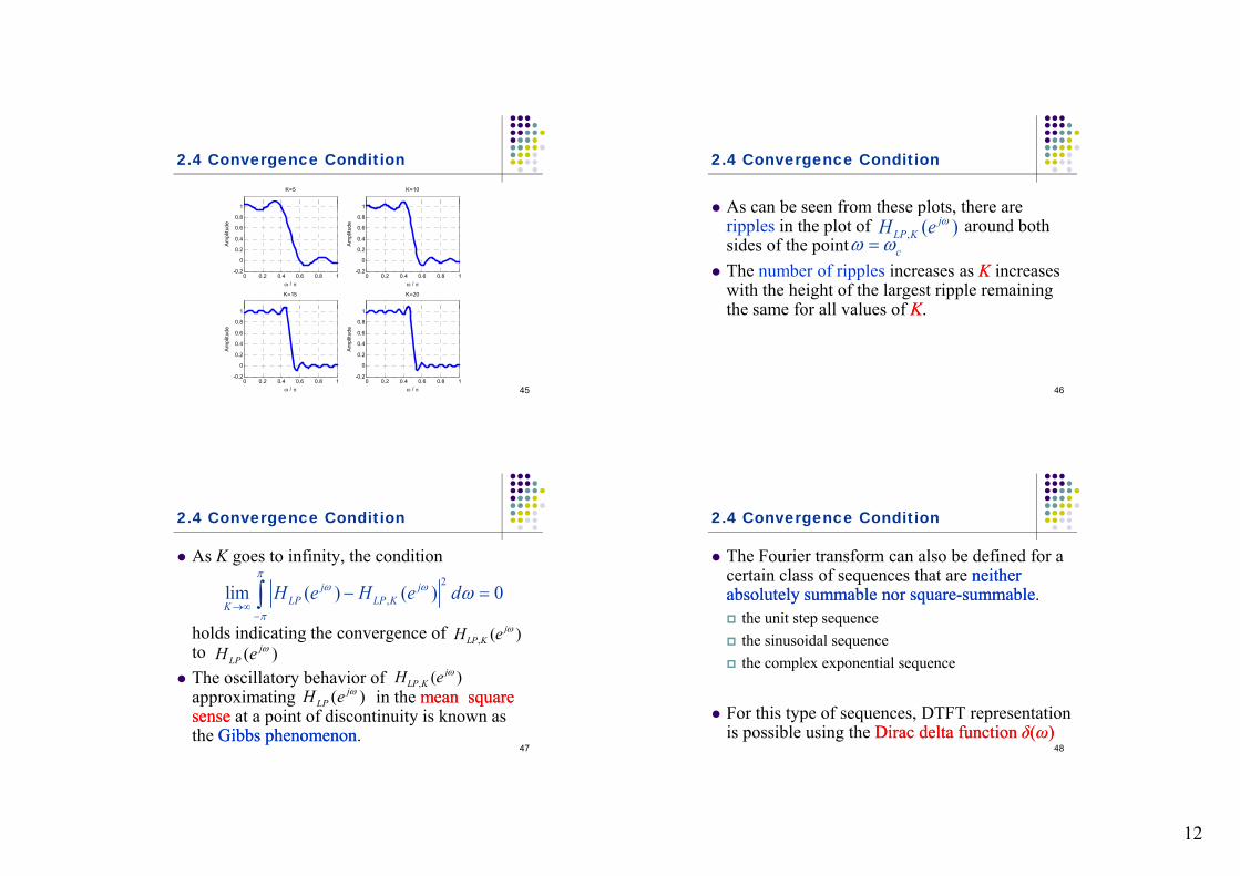
The meanmean--square convergencesquare convergence property of the The meanmean--square convergence square convergence property of the sequence can be further illustrated by examining the plot of the function

[ ]LPh n

,sin

( )K

j j ncLP K

n K

nH e e

n

44

for various values of KK as shown next

12


1

K=5

1

K=10

0 0.2 0.4 0.6 0.8 1-0.2

0

0.2

0.4

0.6

0.8

/

Am

plitu

de

0 0.2 0.4 0.6 0.8 1-0.2

0

0.2

0.4

0.6

0.8

/

Am

plitu

de

K=15 K=20

450 0.2 0.4 0.6 0.8 1

-0.2

0

0.2

0.4

0.6

0.8

1

/

Am

plitu

de

0 0.2 0.4 0.6 0.8 1-0.2

0

0.2

0.4

0.6

0.8

1

/

Am

plitu

de


As can be seen from these plots there are As can be seen from these plots, there are ripples in the plot of around both sides of the point

The number of ripples increases as KK increases with the height of the largest ripple remaining the same for all values of KK

, ( )jLP KH e

c

46

the same for all values of KK.


As K goes to infinity, the condition

holds indicating the convergence of to

2

,lim ( ) ( ) 0j jLP LP KK

H e H e d

, ( )jLP KH e

( )jLPH e

47

The oscillatory behavior of approximating in the mean square mean square sensesense at a point of discontinuity is known as the Gibbs phenomenonGibbs phenomenon.

, ( )jLP KH e

( )jLPH e


The Fourier transform can also be defined for a certain class of sequences that are neither neither absolutely absolutely summablesummable nor squarenor square--summablesummable. the unit step sequence the sinusoidal sequence the complex exponential sequence

48

the complex exponential sequence

For this type of sequences, DTFT representation is possible using the Dirac delta function Dirac delta function δδ((ωω))

13


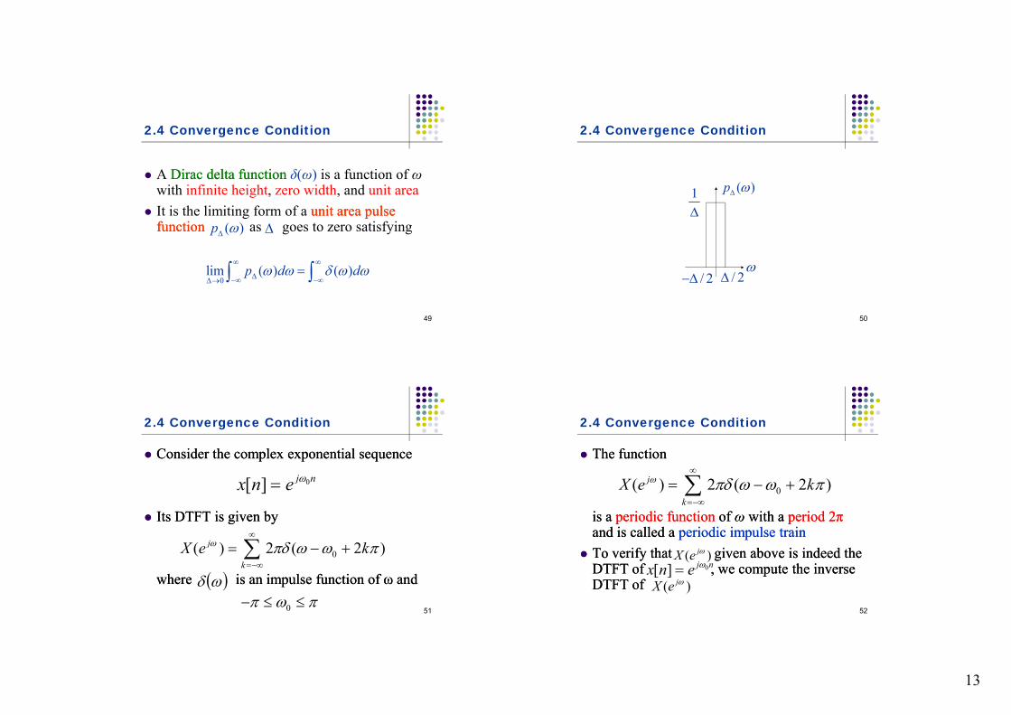
A Di d lt f tiDi d lt f ti δ( ) i f ti f A Dirac delta functionDirac delta function δ(ω) is a function of ωwith infinite height, zero width, and unit area

It is the limiting form of a unit area pulse unit area pulse functionfunction as goes to zero satisfying( )p

49

0lim ( ) ( )p d d


( )p 1

50

/ 2 / 2


Consider the complex exponential sequenceConsider the complex exponential sequence

Its DTFT is given byIts DTFT is given by

0[ ] j nx n e

( ) 2 ( 2 )jX k

51

where is an impulse function of ω andwhere is an impulse function of ω and

0( ) 2 ( 2 )j

kX e k

0


The functionThe function

is a is a periodic functionperiodic function of of ωω with a with a period 2π period 2π and is called a and is called a periodic impulse trainperiodic impulse train

0( ) 2 ( 2 )j

k

X e k

52

To verify that To verify that given above is indeed the given above is indeed the DTFT ofDTFT of , we compute the inverse , we compute the inverse DTFT ofDTFT of

( )jX e

0[ ] j nx n e ( )jX e

14


ThusThus

0

0 0

0

0

1[ ] 2 ( 2 )2

2 ( )

j n

k

j n j n

x n k e d

e d e

53

where we have used the sampling property of where we have used the sampling property of the impulse functionthe impulse function

0( )

Commonly Used DTFT Pairs

54

3 DTFT Computation Using MATLAB

The Signal Processing Toolbox Signal Processing Toolbox in Matlab g gg gincludes a number of M-files to aid in the DTFT-based analysis of discrete-time signals.

Specifically, the functions that can be used are freqzfreqz, absabs, angleangle, and unwrapunwrap.

In addition the built in Matlab functions realreal

55

In addition, the built-in Matlab functions realrealand imagimag are also useful in some applications.


Th f ti ff b d t t The function freqzfreqz can be used to compute the values of the DTFT of a sequence, described as a rational function in the form of

- -

0 1- -

0 1

j j Mj M

j j NN

p p e p eX ed d e d e

56

at a prescribed set of discrete frequency points ω= ωl .

0 1 Nd d e d e

15


For example, the statement H= freqz(num,den,ω)

returns the frequency response values as a vector H of a DTFT defined in terms of the vectors num and den containing the coefficients {pi} and {di} , respectively at a

57

coefficients {pi} and {di} , respectively at a prescribed set of frequencies between 0 and 2πgiven by the vector ω.

For example p=[0.008 －0.033 0.05 －0.033 0.008] d=[1 2.37 2.7 1.6 0.41]


0 5

1Real part

0 5

1Imaginary part

0 0.2 0.4 0.6 0.8 1-1

-0.5

0

0.5

/

Ampl

itude

0 0.2 0.4 0.6 0.8 1-1

-0.5

0

0.5

/

Ampl

itude

0.8

1Magnitude Spectrum

de

2

4Phase Spectrum

dian

s

58

0 0.2 0.4 0.6 0.8 10

0.2

0.4

0.6

/

Mag

nitu

d

0 0.2 0.4 0.6 0.8 1-4

-2

0

/

Phas

e, ra

d

ExerciseExercise：： Program 3_1.mProgram 3_1.m

4.1 DTFT Theorems

LinearityLinearity TimeTime--ReversalReversal

ShiftingShifting (in time and in frequency domain) [ ] jg n G e

0[ ] j n jg n n e G e

59

00[ ] j jg n n e G e

0 0( )[ ]j n je g n G e

4.1 DTFT Theorems

DifferentiationDifferentiation

ConvolutionConvolution (in time and in frequency domain)

[ ]

jdG eng n j

d

60

g[ ] [ ] j jn h n G e H e

( - )1[ ] [ ]2

j jg n h n G e H e d

16

4.1 DTFT Theorems

Area TheoremArea Theorem (simple but useful)( p )

Parseval’sParseval’s TheoremTheorem

0

-[ ]j

nX e x n

-

1[0]2

jx X e d

* *1[ ] [ ] j jg n h n G e H e d

61

CorollaryCorollary——Energy is preserved

-

-[ ] [ ]

2ng n h n G e H e d

22 1[ ]2

j

nx n X e d

4.1 DTFT Theorems

Symmetry Relations (DTFT pairs)Symmetry Relations (DTFT pairs) Symmetry Relations (DTFT pairs)Symmetry Relations (DTFT pairs)

For an arbitrary real sequencereal sequence

[ ] ( )jre csx n X e [ ] ( )j

im cajx n X e

Re[ ] ( )jcsx n X e Im[ ] ( )j

cax n jX e

*( ) ( )j jX e X e

62

Corollary Corollary ( ) ( )j jX e X e

Re ( )jX e ( )jX e Im ( )jX e arg ( )jX e

Type of Property Sequence DTFT

ng jeG nh jeH

Linearity

Time-shifting

Frequency-shifting

Differentiation in

nhng

0nng

nge nj 0

nng

jj eHeG

jnj eGe 0

0jeG

edGjj

deHeGnhng jj

n

**

21

frequency

Convolution

Modulation

Parseval’s relation

63

nng

nhng *

nhng

d

j

jj eHeG

deHeG jj

21

4.1 DTFT Theorems

ExampleExamplepp

Determine the DFT Y(ejω) of y[n]=(n+1)anu[n](|a|<1)

Step 1: Let x[n]=anu[n] . Thereforey[n]=nx[n]+x[n]

64

Step 2: Calculate the DTFT X(ejω)

-

1( )1

jjX e

ae

17

4.1 DTFT Theorems

St 3 C l l t th DTFT f [ ]Step 3: Calculate the DTFT of nx[n]

Step 4: Calculate the DTFT Y(ejω) of y[n] 2 2

( )

1 1

j j j

j j

dX e aje aej jd ae ae

1 1j

65

2 2

1 111 1

jj

jj j

aeY eaeae ae

4.1 DTFT Theorems

ExampleExamplepp

Determine the DTFT V(ejω) of the sequence v[n] defined by

Using the time shifting property we observe0 1 0 1[ ] [ 1] [ ] [ 1]d v n d v n p n p n

66

Using the time-shifting property, we observe that the DTFT of is and the DTFT of is

[ 1]n [ 1]v n

je

( )j je V e

4.1 DTFT Theorems

Using the linearity property we then obtain g y p p ythe frequency-domain representation of

as

S l i h b i

0 1 0 1[ ] [ 1] [ ] [ 1]d v n d v n p n p n

0 1 0 1( ) ( )j j j jd V e d e V e p p e

67

• Solving the above equation we get

0 1

0 1

( )j

jj

p p eV e

d d e

4.2 Linear Convolution Using DTFT

A di t th l ti th According to the convolution theorem

An implication of this result is that the linear convolution y[n] of the sequences x[n] and

[ ] [ ] [ ] j j jy n x n h n Y e X e H e

68

convolution y[n] of the sequences x[n] and h[n] can be performed as follows:

18

j j

4.2 Linear Convolution Using DTFT

Step 1: Compute the DTFTs X(ejω) and H(ejω)of the sequences x[n] and h[n], respectively.

Step 2: Form the DTFT Y(ejω)= X(ejω)H(ejω)Step 3: Compute the IDTFT y[n] of Y(ejω)

X( j )

69

DTFT

DTFT× IDTFT

x[n]

h[n]

X(ejω)

H(ejω)

Y(ejω) y[n]

5 Energy Density Spectrum

The total energy of a finite-energy sequence g[n] is given by

From Parseval’s relation Parseval’s relation we observe that

2[ ]gn

g n

70

22 1[ ]2

jg

n

g n G e d


The quantity

is called the energy density spectrumenergy density spectrum

The area nder this c r e in the range

2j jggS e G e

71

The area under this curve in the range divided by is the energy of the sequence

2


Recall that the auto correlation sequence r [l] Recall that the auto-correlation sequence rgg[l]of g[n] can be expressed as

As we know that the DTFT of g[－ l] is G(e－jω), h f h DTFT f i i b

[ ] [ ] [ ( )] [ ] [ ]ggn

r l g n g l n g l g l

[ ] [ ]l l

72

therefore, the DTFT of is given by |G(ejω)|2, where we have used the fact that for afor areal sequencereal sequence g[n], G(e－jω)=G*(ejω)

[ ] [ ]g l g l

19


As a result, the energy density spectrum Sgg(ejω) of a real sequence real sequence g[n] can be computed by taking the DTFT of its auto-correlation sequence rgg(l), i.e.,

l

73

[ ]j j lgg gg

lS e r l e


ExampleExample Compute the energy of the sequence

Heresin

[ ] ,cLP

nh n n

n

22 1[ ] jLP LPh n H e d

74

where

-

[ ]2LP LP

n

1, 00,

cjLP

c

H e


Therefore, Compute the energy of the sequence

2

-

1( )2

c

c

cLP

nh n d

75

Hence, hLP(n) is a finitefinite--energy sequenceenergy sequence

6 Band-limited Discrete-Time Signals

Discrete time signal is a periodic function of Discrete-time signal is a periodic function of ω with a period 2π.

A fullfull--bandband, finite-energy, discrete-time signal has a spectrum occupying the whole whole frequency rangefrequency range −π≤ω< π

76

q y gq y g A bandband--limitedlimited discrete-time signal has a

spectrum that is limited to a portion of the a portion of the frequency rangefrequency range −π ≤ ω < π

20


An ideal bandideal band limitedlimited signal has a spectrum An ideal bandideal band--limitedlimited signal has a spectrum that is zero outside a finite frequency range ω 0≤ ωa≤| ω|≤ ωb ≤ π , that is

0, 0( )

0aj

b

X e

77

However, an ideal band-limited signal cannot be generated in practice (WhyWhy?)?)

0, b


B dB d li it d i lli it d i l l ifi d di BandBand--limited signals limited signals are classified according to the frequency range where most of the most of the signal’s energy is concentratedsignal’s energy is concentrated

A lowpasslowpass, discrete-time signal has a spectrum occupying the frequency range

78

occupying the frequency range -π< -ωp ≤ |ω|≤ ωp<π

where ωp is called the bandwidthbandwidth of the signal


A highpasshighpass, discrete-time signal has a spectrum occupying the frequency range ωp ≤ |ω|<π where the bandwidth bandwidth of the signal is from π-ωp

A bandpassbandpass, discrete-time signal has a

79

spectrum occupying the frequency range 0< ωL ≤ |ω| ≤ ωH < π where ωH− ωL is the bandwidthbandwidth

A precise definition of the bandwidth depends on applications: 80% of the energy

Date post:	13-Jan-2020
Category:	Documents
Upload:	others
View:	1 times
Download:	0 times

Chapter 3 Two major topics of this chapter: Ch t 3Chapter...

Documents