Page 1
R. G
ross
© W
alth
er-
Me
ißn
er-
Inst
itu
t (2
00
1 -
20
15
)
TT1-Chap2 - 1
Chapter 3
3. Phenomenological Models of Superconductivity
3.1 London Theory
3.1.1 The London Equations
3.2 Macroscopic Quantum Model of Superconductivity
3.2.1 Derivation of the London Equations
3.2.2 Fluxoid Quantization
3.2.3 Josephson Effect
3.3 Ginzburg-Landau Theory
3.3.1 Type-I and Type-II Superconductors
3.3.2 Type-II Superconductors: Upper and Lower Critical Field
3.3.3 Type-II Superconductors: Shubnikov Phase and Flux Line Lattice
3.3.4 Type-II Superconductors: Flux Lines
Page 2
R. G
ross
© W
alth
er-
Me
ißn
er-
Inst
itu
t (2
00
1 -
20
15
)
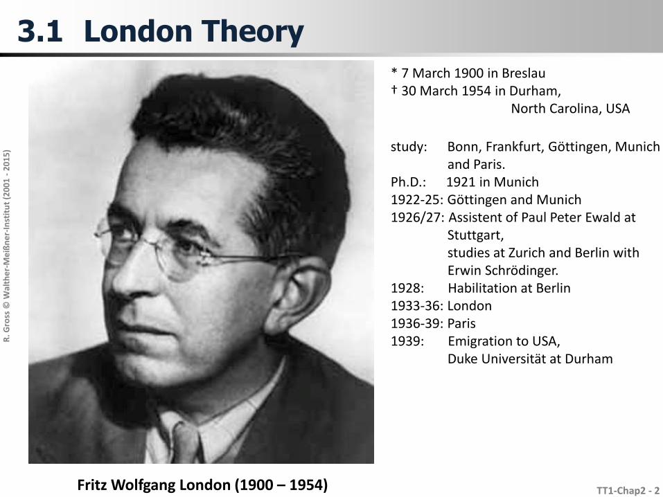
TT1-Chap2 - 2Fritz Wolfgang London (1900 – 1954)
3.1 London Theory
* 7 March 1900 in Breslau † 30 March 1954 in Durham,
North Carolina, USA
study: Bonn, Frankfurt, Göttingen, Munichand Paris.
Ph.D.: 1921 in Munich1922-25: Göttingen and Munich1926/27: Assistent of Paul Peter Ewald at
Stuttgart, studies at Zurich and Berlin withErwin Schrödinger.
1928: Habilitation at Berlin 1933-36: London1936-39: Paris1939: Emigration to USA,
Duke Universität at Durham
Page 3
R. G
ross
© W
alth
er-
Me
ißn
er-
Inst
itu
t (2
00
1 -
20
15
)
TT1-Chap2 - 3
Heinz and Fritz London
3.1 London Theory
Page 4
R. G
ross
© W
alth
er-
Me
ißn
er-
Inst
itu
t (2
00
1 -
20
15
)
TT1-Chap2 - 4
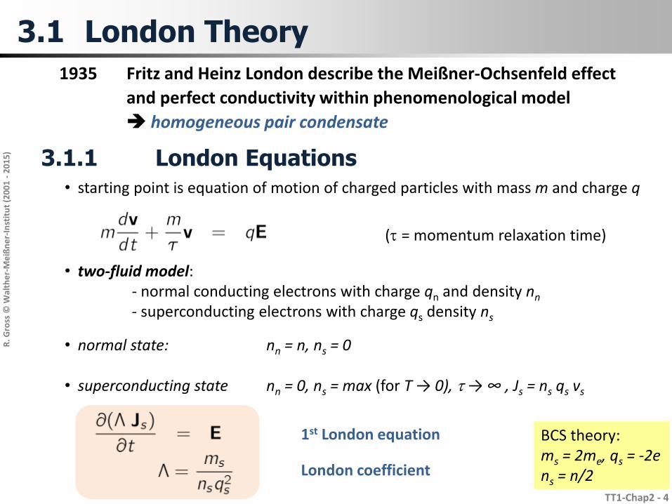
3.1 London Theory
1935 Fritz and Heinz London describe the Meißner-Ochsenfeld effect
and perfect conductivity within phenomenological model
homogeneous pair condensate
• starting point is equation of motion of charged particles with mass m and charge q
(t = momentum relaxation time)
• two-fluid model: - normal conducting electrons with charge qn and density nn
- superconducting electrons with charge qs density ns
• normal state: nn = n, ns = 0
• superconducting state nn = 0, ns = max (for T → 0), t → ∞ , Js = ns qs vs
1st London equation
London coefficient
BCS theory:ms = 2me, qs = -2ens = n/2
3.1.1 London Equations
Page 5
R. G
ross
© W
alth
er-
Me
ißn
er-
Inst
itu
t (2
00
1 -
20
15
)
TT1-Chap2 - 5
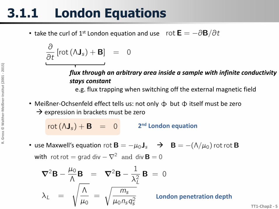
3.1.1 London Equations
• take the curl of 1st London equation and use
flux through an arbitrary area inside a sample with infinite conductivitystays constant
e.g. flux trapping when switching off the external magnetic field
• Meißner-Ochsenfeld effect tells us: not only but itself must be zero expression in brackets must be zero
2nd London equation
• use Maxwell‘s equation
with
London penetration depth
Page 6
R. G
ross
© W
alth
er-
Me
ißn
er-
Inst
itu
t (2
00
1 -
20
15
)
TT1-Chap2 - 6
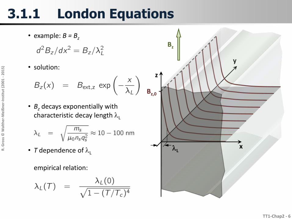
3.1.1 London Equations
• example: B = Bz
y
Bz,0
Bz
z
xlL
• solution:
• Bz decays exponentially withcharacteristic decay length lL
• T dependence of lL
empirical relation:
Page 7
R. G
ross
© W
alth
er-
Me
ißn
er-
Inst
itu
t (2
00
1 -
20
15
)
TT1-Chap2 - 7
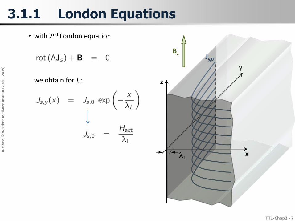
3.1.1 London Equations
• with 2nd London equation
we obtain for Js:
y
z
Bz
xlL
Jy,0
Page 8
R. G
ross
© W
alth
er-
Me
ißn
er-
Inst
itu
t (2
00
1 -
20
15
)
TT1-Chap2 - 8
3.1.1 London Equations
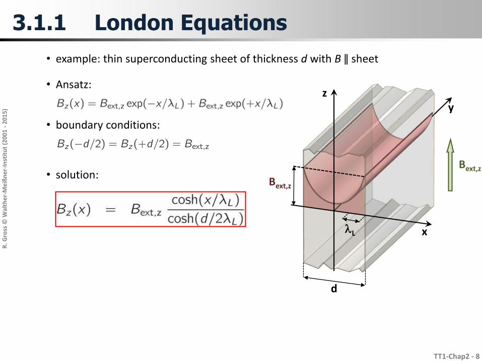
• example: thin superconducting sheet of thickness d with B ǁ sheet
• Ansatz:
y
Bext,z
Bext,z
x
z
lL
d
• boundary conditions:
• solution:
Page 9
R. G
ross
© W
alth
er-
Me
ißn
er-
Inst
itu
t (2
00
1 -
20
15
)
TT1-Chap2 - 9
3.1.1 London Equations
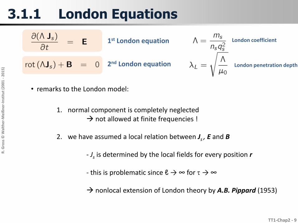
• remarks to the London model:
1. normal component is completely neglected not allowed at finite frequencies !
2. we have assumed a local relation between Js , E and B
- Js is determined by the local fields for every position r
- this is problematic since ℓ → ∞ for t → ∞
nonlocal extension of London theory by A.B. Pippard (1953)
1st London equation London coefficient
2nd London equation London penetration depth
Page 10
R. G
ross
© W
alth
er-
Me
ißn
er-
Inst
itu
t (2
00
1 -
20
15
)
TT1-Chap2 - 10
3.2 SC as Macroscopic Quantum Phenomenon
• more solid derivation of London equations by assuming that superconductor can bedesrcribed by a macroscopic wave function
- Fritz London (> 1948)- derived London equations from basic quantum mechanical concepts
• basic assumption of macroscopic quantum model of superconductivity
complete entity of all superconducting electrons can be described by macroscopicwave function
amplitude phase
• hypothesis can be proven by BCS theory (discussed later)
• normalization condition: volume integral over |y|² is equal to the number Ns of superconducting electrons
Page 11
R. G
ross
© W
alth
er-
Me
ißn
er-
Inst
itu
t (2
00
1 -
20
15
)
TT1-Chap2 - 11
• general relations in electrodynamics:
electric field:
flux density:
A = vector potentialf = scalar potential
• canonical momentum:
3.2 SC as Macroscopic Quantum Phenomenon
• electrical current is driven by gradient of electrochemical potential:
• kinematic momentum:
Page 12
R. G
ross
© W
alth
er-
Me
ißn
er-
Inst
itu
t (2
00
1 -
20
15
)
TT1-Chap2 - 12
• Schrödinger equation for charged particle:
electro-chemical potential
• insert macroscopic wave-function (Madelung transformation)
replacements: Y y, q qs, mms
3.2 SC as Macroscopic Quantum Phenomenon
• calculation yields after splitting up into real and imaginary part two fundamental equations
- current-phase relation: connects supercurrent density with gauge invariant phase gradient
- energy-phase gradient: connects energy with time derivative of the phase
Page 13
R. G
ross
© W
alth
er-
Me
ißn
er-
Inst
itu
t (2
00
1 -
20
15
)
TT1-Chap2 - 13
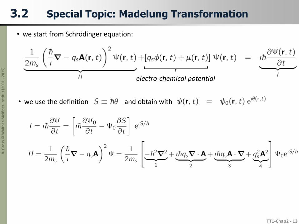
3.2 Special Topic: Madelung Transformation
• we start from Schrödinger equation:
electro-chemical potential
• we use the definition and obtain with
Page 14
R. G
ross
© W
alth
er-
Me
ißn
er-
Inst
itu
t (2
00
1 -
20
15
)
TT1-Chap2 - 14
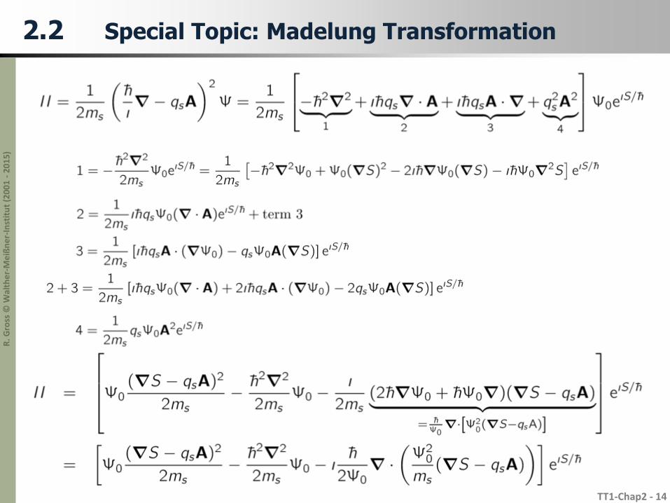
2.2 Special Topic: Madelung Transformation
Page 15
R. G
ross
© W
alth
er-
Me
ißn
er-
Inst
itu
t (2
00
1 -
20
15
)
TT1-Chap2 - 15
3.2 Special Topic: Madelung Transformation
• equation for real part:
energy-phase relation (term of order ²ns is usually neglected)
∆
Page 16
R. G
ross
© W
alth
er-
Me
ißn
er-
Inst
itu
t (2
00
1 -
20
15
)
TT1-Chap2 - 16
• interpretation of energy-phase relation
3.2 Special Topic: Madelung Transformation
corresponds to action
in the quasi-classical limes the energy-phase-relation becomesthe Hamilton-Jacobi equation
Page 17
R. G
ross
© W
alth
er-
Me
ißn
er-
Inst
itu
t (2
00
1 -
20
15
)
TT1-Chap2 - 17
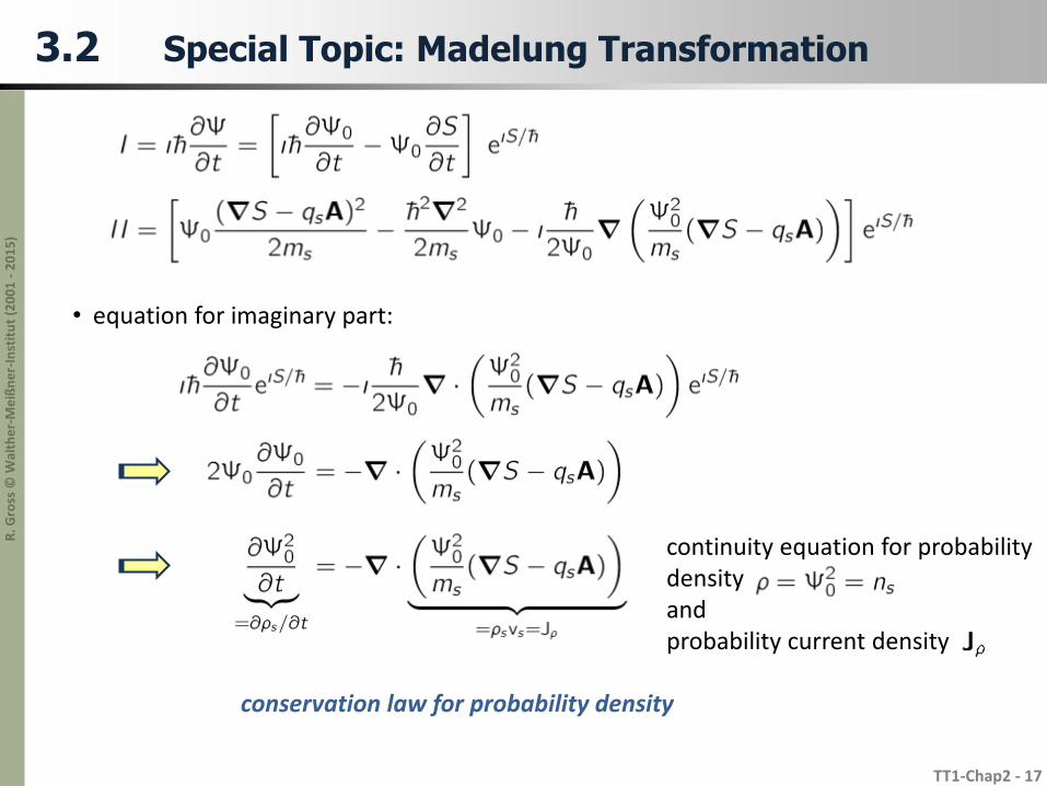
• equation for imaginary part:
3.2 Special Topic: Madelung Transformation
continuity equation for probabilitydensityandprobability current density
conservation law for probability density
Page 18
R. G
ross
© W
alth
er-
Me
ißn
er-
Inst
itu
t (2
00
1 -
20
15
)
TT1-Chap2 - 18
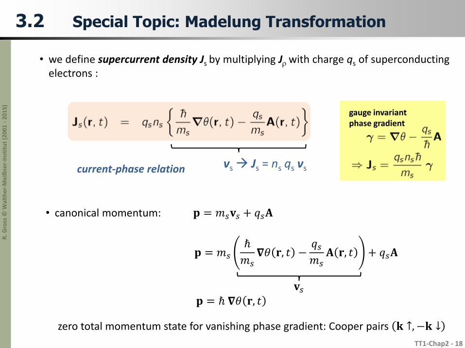
3.2 Special Topic: Madelung Transformation
• we define supercurrent density Js by multiplying Jr with charge qs of superconductingelectrons :
vs Js = ns qs vs
gauge invariant phase gradient
current-phase relation
• canonical momentum: 𝐩 = 𝑚𝑠𝐯𝑠 + 𝑞𝑠𝐀
𝐩 = 𝑚𝑠
ℏ
𝑚𝑠𝛁𝜃 𝐫, 𝑡 −
𝑞𝑠
𝑚𝑠𝐀 𝐫, 𝑡 + 𝑞𝑠𝐀
𝐩 = ℏ 𝛁𝜃 𝐫, 𝑡
𝐯𝑠
zero total momentum state for vanishing phase gradient: Cooper pairs 𝐤 ↑, −𝐤 ↓
Page 19
R. G
ross
© W
alth
er-
Me
ißn
er-
Inst
itu
t (2
00
1 -
20
15
)
TT1-Chap2 - 19
• energy-phase relation
• supercurrent density-phase relation
(i) superconductor with Cooper pairs of charge qs = -2e
(ii) neutral Bose superfluid, e.g. 4He
(iii) neutral Fermi superfluid, e.g. 3He
equations (1) and (2) have general validity for charged and uncharged superfluids
(London parameter)
1
2
we use equations (1) and (2) to derive London equations
3.2 SC as Macroscopic Quantum Phenomenon
• note: k drops out !!
Page 20
R. G
ross
© W
alth
er-
Me
ißn
er-
Inst
itu
t (2
00
1 -
20
15
)
TT1-Chap2 - 20
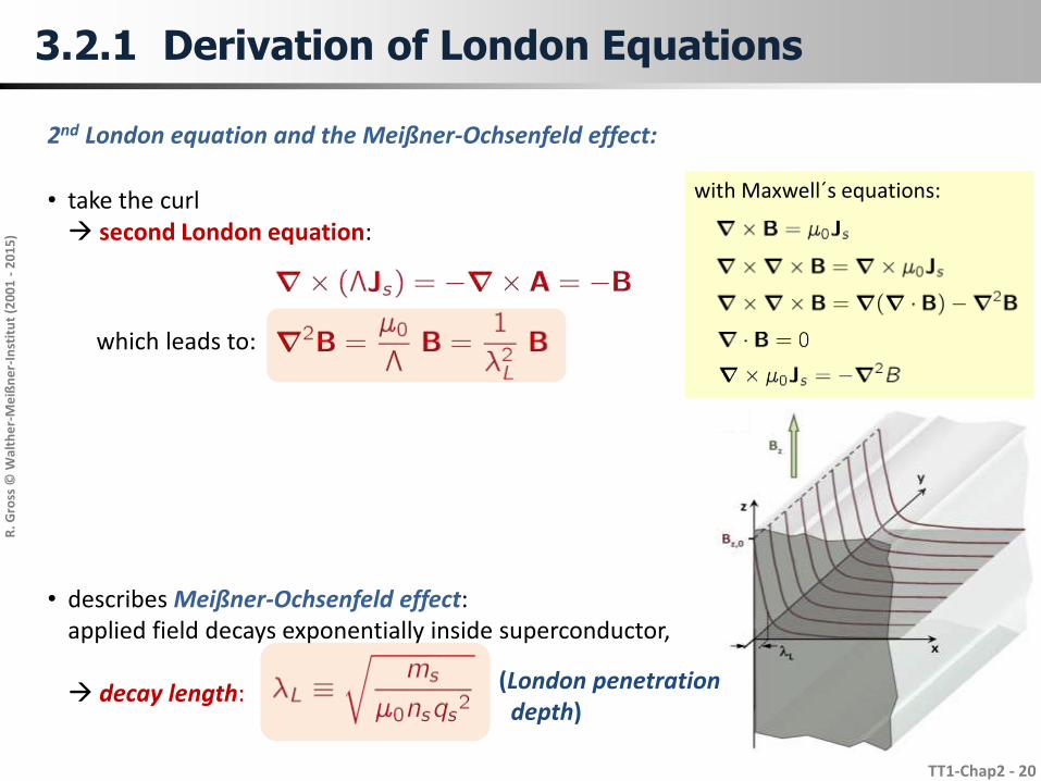
• take the curl second London equation:
which leads to:
• describes Meißner-Ochsenfeld effect: applied field decays exponentially inside superconductor,
decay length:
with Maxwell´s equations:
(London penetration depth)
2nd London equation and the Meißner-Ochsenfeld effect:
3.2.1 Derivation of London Equations
Page 21
R. G
ross
© W
alth
er-
Me
ißn
er-
Inst
itu
t (2
00
1 -
20
15
)
TT1-Chap2 - 21
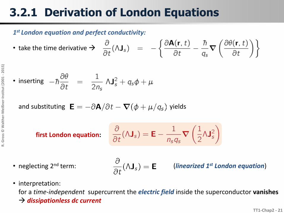
1st London equation and perfect conductivity:
• take the time derivative
first London equation:
• neglecting 2nd term:
• interpretation: for a time-independent supercurrent the electric field inside the superconductor vanishes dissipationless dc current
(linearized 1st London equation)
• inserting
and substituting yields
3.2.1 Derivation of London Equations
Page 22
R. G
ross
© W
alth
er-
Me
ißn
er-
Inst
itu
t (2
00
1 -
20
15
)
TT1-Chap2 - 22
3.2.1 London Equations - Summary
• energy-phase relation
• supercurrent density-phase relation (London parameter)
1
2
• take the curl
which leads to:
2nd London equation and the Meißner-Ochsenfeld effect:
2nd Londonequation
1st London equation and perfect conductivity:
• take the time derivative
which leads to: 1st Londonequation
Page 23
R. G
ross
© W
alth
er-
Me
ißn
er-
Inst
itu
t (2
00
1 -
20
15
)
TT1-Chap2 - 23
3.2.1 Derivation of London Equations
• the assumption that the superconducting state can be described by a macroscopicwave function leads to a general expression for the supercurrent density Js
• London equations can be directly derived from the general expression for thesupercurrent density Js
• London equations together with Maxwell‘s equations describe the behavior ofsuperconductors in electric and magnetic fields
• London equations cannot be used for the description of spatially inhomogeneoussituations Ginzburg-Landau theory
• London equations can be used for the description of time-dependent situations Josephson equations
Page 24
R. G
ross
© W
alth
er-
Me
ißn
er-
Inst
itu
t (2
00
1 -
20
15
)
TT1-Chap2 - 24
• Processes that could cause a decay of Js (plausibility consideration):
example: Fermi sphere in two dimensions in the kxky – plane
• T = 0: all states inside the Fermi circle are occupied• current in x-direction shift of Fermi circle along kx by ±kx
• normal state: relaxation into states with lower energy (obeying Pauli principle) centered Fermi sphere, current relaxes
• superconducting state: Cooper pairs with the same center of mass moment (discussion later)
only scattering around the sphere no decay of supercurrent
normal state superconducting state
3.2.1 Derivation of London Equations
Page 25
R. G
ross
© W
alth
er-
Me
ißn
er-
Inst
itu
t (2
00
1 -
20
15
)
TT1-Chap2 - 25
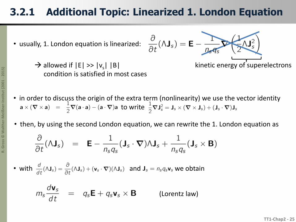
kinetic energy of superelectrons
• usually, 1. London equation is linearized:
allowed if |E| >> |vs| |B|condition is satisfied in most cases
3.2.1 Additional Topic: Linearized 1. London Equation
• in order to discuss the origin of the extra term (nonlinearity) we use the vector identityto write
• then, by using the second London equation, we can rewrite the 1. London equation as
• with and we obtain
(Lorentz law)
Page 26
R. G
ross
© W
alth
er-
Me
ißn
er-
Inst
itu
t (2
00
1 -
20
15
)
TT1-Chap2 - 26
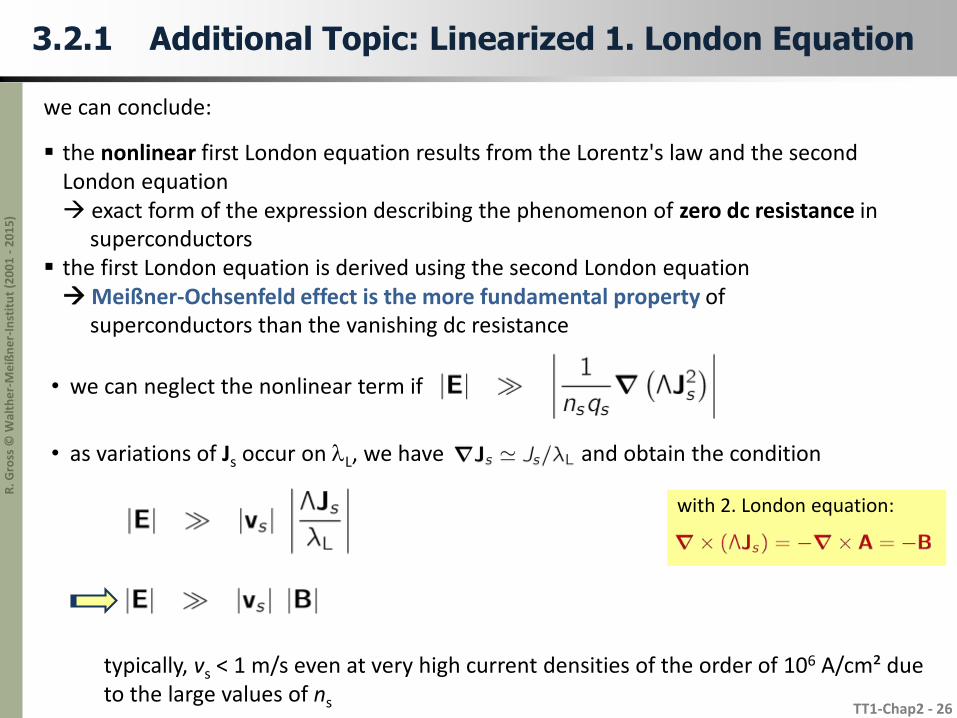
we can conclude:
the nonlinear first London equation results from the Lorentz's law and the second London equation exact form of the expression describing the phenomenon of zero dc resistance in
superconductors the first London equation is derived using the second London equationMeißner-Ochsenfeld effect is the more fundamental property of
superconductors than the vanishing dc resistance
3.2.1 Additional Topic: Linearized 1. London Equation
• we can neglect the nonlinear term if
• as variations of Js occur on lL, we have and obtain the condition
with 2. London equation:
typically, vs < 1 m/s even at very high current densities of the order of 106 A/cm² due to the large values of ns
Page 27
R. G
ross
© W
alth
er-
Me
ißn
er-
Inst
itu
t (2
00
1 -
20
15
)
TT1-Chap2 - 27
3.2.1 Additional Topic: The London Gauge
• 1. London equation:
• frequently, we have no conversion of Js in Jn or no supercurrent flow throuh sample surface
• in some cases it is convenient to choose a special gauge often used: The London Gauge
• if the macroscopic wavefunction is single valued (this is the case for a simply connected superconductor containing no flux) we can choose such that
a vector potential that satisfies is said to be in the London gauge
everywhere
Page 28
R. G
ross
© W
alth
er-
Me
ißn
er-
Inst
itu
t (2
00
1 -
20
15
)
TT1-Chap2 - 28
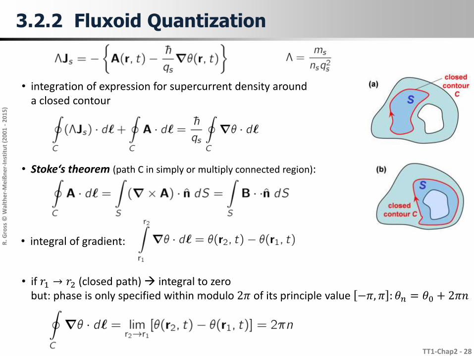
• Stoke‘s theorem (path C in simply or multiply connected region):
• if 𝑟1 → 𝑟2 (closed path) integral to zerobut: phase is only specified within modulo 2𝜋 of its principle value −𝜋, 𝜋 : 𝜃𝑛 = 𝜃0 + 2𝜋𝑛
• integration of expression for supercurrent density arounda closed contour
3.2.2 Fluxoid Quantization
• integral of gradient:
Page 29
R. G
ross
© W
alth
er-
Me
ißn
er-
Inst
itu
t (2
00
1 -
20
15
)
TT1-Chap2 - 29
• then:
• flux quantum:
fluxoid is quantized in units of F0
• quantization condition holds for all contour linesincluding contour that can be shrunk to single point
𝑟1 = 𝑟2: 𝑟1𝑟2 𝛁𝜃 ⋅ 𝑑ℓ = 0
• contour line can no longer be shrunk to single point inclusion of nonsuperconducting region in contour 𝑟1 = 𝑟2: we have built in „memory“ in integration path
𝑛 ≠ 0 possible, 𝑟1𝑟2 𝛁𝜃 ⋅ 𝑑ℓ =2𝜋𝑛
3.2.2 Fluxoid Quantization
Page 30
R. G
ross
© W
alth
er-
Me
ißn
er-
Inst
itu
t (2
00
1 -
20
15
)
TT1-Chap2 - 30
rr
Js
screeningcurrent oninner wall
Hextmagneticflux
Js
3.2.2 Fluxoid Quantization
screeningcurrent onouter wall
Page 31
R. G
ross
© W
alth
er-
Me
ißn
er-
Inst
itu
t (2
00
1 -
20
15
)
TT1-Chap2 - 31
• Fluxoid Quantization:total flux = external applied flux + flux generated by induced supercurrentmust have discrete values
• Flux Quantization:- superconducting cylinder, wall much thicker than 𝜆𝐿
- application of small magnetic field at 𝑇 < 𝑇𝑐 screening currents, no flux inside
application of 𝐵cool during cool down: screening current on outer and inner wall amount of flux trapped in cylinder: satisfies fluxoid quantization condition wall thickness ≫ 𝜆L: closed contour deep inside with 𝐽𝑠 = 0 then:
remove field after cooling down trapped flux = integer multiple of flux quantum
flux quantization
3.2.2 Fluxoid Quantization
Page 32
R. G
ross
© W
alth
er-
Me
ißn
er-
Inst
itu
t (2
00
1 -
20
15
)
TT1-Chap2 - 32
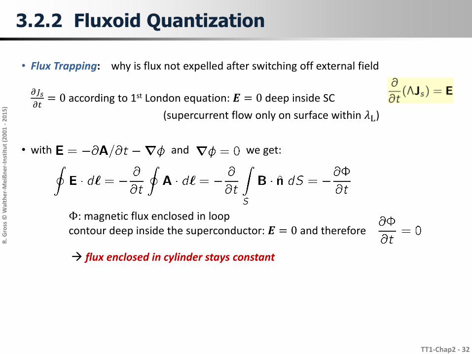
• Flux Trapping: why is flux not expelled after switching off external field
𝜕𝐽𝑠
𝜕𝑡= 0 according to 1st London equation: 𝑬 = 0 deep inside SC
(supercurrent flow only on surface within 𝜆L)
• with and we get:
Φ: magnetic flux enclosed in loopcontour deep inside the superconductor: 𝑬 = 0 and therefore
flux enclosed in cylinder stays constant
3.2.2 Fluxoid Quantization
Page 33
R. G
ross
© W
alth
er-
Me
ißn
er-
Inst
itu
t (2
00
1 -
20
15
)
TT1-Chap2 - 33
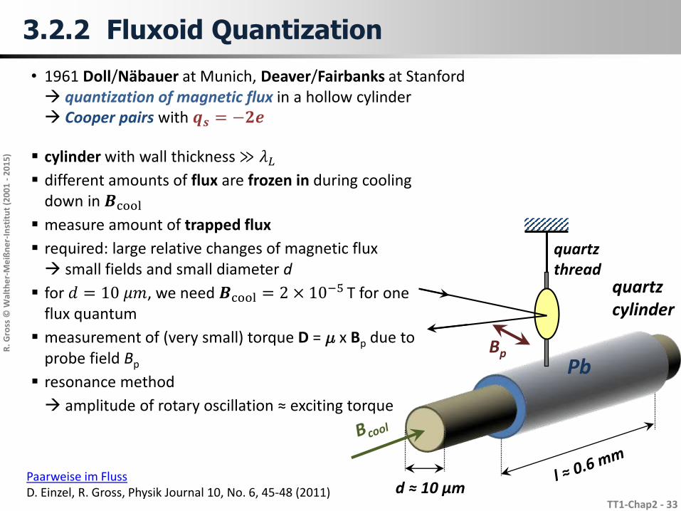
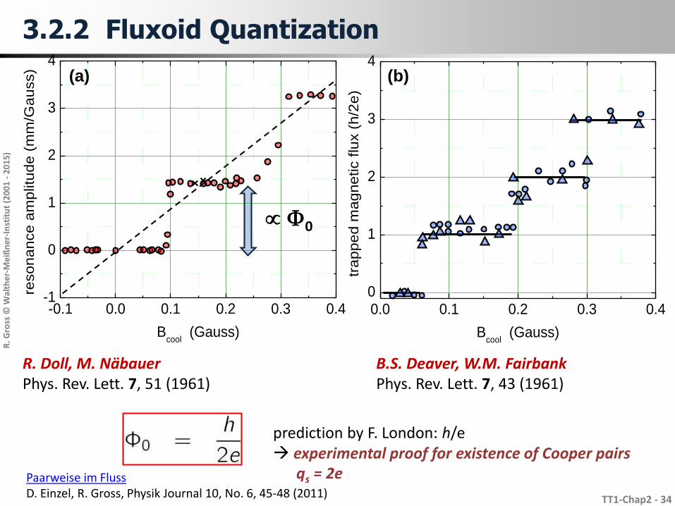
• 1961 Doll/Näbauer at Munich, Deaver/Fairbanks at Stanford quantization of magnetic flux in a hollow cylinder Cooper pairs with 𝒒𝒔 = −𝟐𝒆
cylinder with wall thickness ≫ 𝜆𝐿
different amounts of flux are frozen in during coolingdown in 𝑩cool
measure amount of trapped flux
required: large relative changes of magnetic flux small fields and small diameter d
for 𝑑 = 10 𝜇𝑚, we need 𝑩cool = 2 × 10⁻⁵ T for oneflux quantum
measurement of (very small) torque D = ¹ x Bp due toprobe field Bp
resonance method
amplitude of rotary oscillation ≈ exciting torque
d ≈ 10 µm
Pb
quartzcylinder
Bp
quartzthread
3.2.2 Fluxoid Quantization
Paarweise im Fluss D. Einzel, R. Gross, Physik Journal 10, No. 6, 45-48 (2011)
Page 34
R. G
ross
© W
alth
er-
Me
ißn
er-
Inst
itu
t (2
00
1 -
20
15
)
TT1-Chap2 - 34
Paarweise im Fluss D. Einzel, R. Gross, Physik Journal 10, No. 6, 45-48 (2011)
3.2.2 Fluxoid Quantization
(a) (b)
R. Doll, M. NäbauerPhys. Rev. Lett. 7, 51 (1961)
B.S. Deaver, W.M. FairbankPhys. Rev. Lett. 7, 43 (1961)
F0
prediction by F. London: h/e experimental proof for existence of Cooper pairs
qs = 2e
-0.1 0.0 0.1 0.2 0.3 0.4-1
0
1
2
3
4
reso
na
nce
am
plitu
de
(m
m/G
au
ss)
Bcool
(Gauss)
0.0 0.1 0.2 0.3 0.40
1
2
3
4
tra
pp
ed
ma
gn
etic f
lux (
h/2
e)
Bcool
(Gauss)
Page 35
R. G
ross
© W
alth
er-
Me
ißn
er-
Inst
itu
t (2
00
1 -
20
15
)
TT1-Chap2 - 35
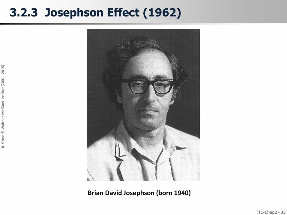
Brian David Josephson (born 1940)
3.2.3 Josephson Effect (1962)
Page 36
R. G
ross
© W
alth
er-
Me
ißn
er-
Inst
itu
t (2
00
1 -
20
15
)
TT1-Chap2 - 36
• what happens if we weakly couple two superconductors?- coupling by tunneling barriers, point contacts, normal conducting layers, etc.- do they form a bound state such as a molecule?- if yes, what is the binding energy?
• B.D. Josephson in 1962 (nobel prize with Esaki and Giaever in 1973)
finite supercurrent at zero applied voltage
oscillation of supercurrent at constant applied voltage
finite binding energy of coupled SCs = Josephson coupling energy
Josephson effects
3.2.3 Josephson Effect
Cooper pairs can tunnel through thin insulating barrierexpectation:- tunneling probability for pairs ∝ 𝑇 2 2
extremely small ∼ 10−4 2
Josephson:- tunneling probability for pairs ∝ 𝑇 2
- coherent tunneling of pairs („tunneling of macroscopic wave function“)
Page 37
R. G
ross
© W
alth
er-
Me
ißn
er-
Inst
itu
t (2
00
1 -
20
15
)
TT1-Chap2 - 37
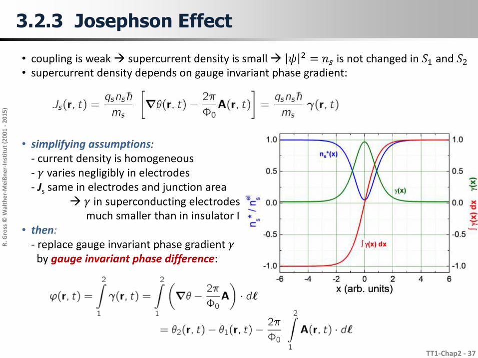
• coupling is weak supercurrent density is small 𝜓 2 = 𝑛𝑠 is not changed in 𝑆1 and 𝑆2
• supercurrent density depends on gauge invariant phase gradient:
• simplifying assumptions:- current density is homogeneous- 𝛾 varies negligibly in electrodes- Js same in electrodes and junction area
𝛾 in superconducting electrodesmuch smaller than in insulator I
• then:- replace gauge invariant phase gradient 𝛾
by gauge invariant phase difference:
3.2.3 Josephson Effect
Page 38
R. G
ross
© W
alth
er-
Me
ißn
er-
Inst
itu
t (2
00
1 -
20
15
)
TT1-Chap2 - 38
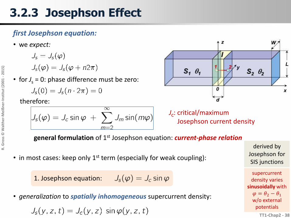
• we expect:
• for Js = 0: phase difference must be zero:
therefore:
Jc: critical/maximumJosephson current density
• in most cases: keep only 1st term (especially for weak coupling):
1. Josephson equation:
• generalization to spatially inhomogeneous supercurrent density:
derived byJosephson forSIS junctions
supercurrent density varies
sinusoidally with𝜑 = 𝜃2 − 𝜃1
w/o externalpotentials
general formulation of 1st Josephson equation: current-phase relation
first Josephson equation:
3.2.3 Josephson Effect
Page 39
R. G
ross
© W
alth
er-
Me
ißn
er-
Inst
itu
t (2
00
1 -
20
15
)
TT1-Chap2 - 39
3.2.3 Josephson Effect
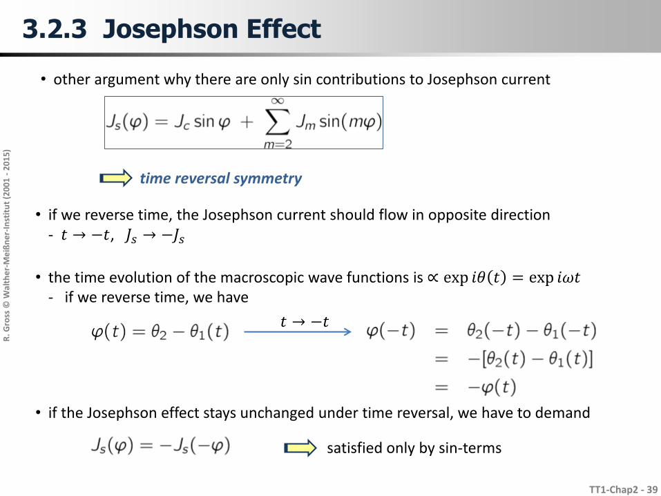
• other argument why there are only sin contributions to Josephson current
time reversal symmetry
• if we reverse time, the Josephson current should flow in opposite direction- 𝑡 → −𝑡, 𝐽𝑠 → −𝐽𝑠
• the time evolution of the macroscopic wave functions is ∝ exp 𝑖𝜃 𝑡 = exp 𝑖𝜔𝑡- if we reverse time, we have
𝑡 → −𝑡
• if the Josephson effect stays unchanged under time reversal, we have to demand
satisfied only by sin-terms
Page 40
R. G
ross
© W
alth
er-
Me
ißn
er-
Inst
itu
t (2
00
1 -
20
15
)
TT1-Chap2 - 40
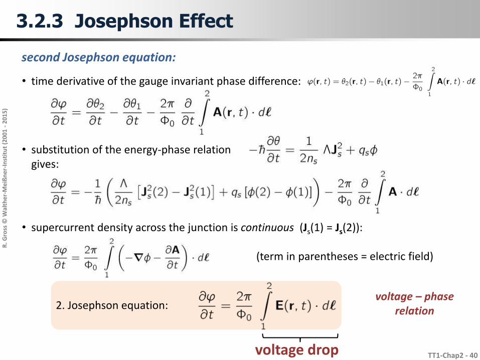
• time derivative of the gauge invariant phase difference:
• substitution of the energy-phase relationgives:
• supercurrent density across the junction is continuous (Js(1) = Js(2)):
2. Josephson equation:
(term in parentheses = electric field)
second Josephson equation:
voltage drop
voltage – phaserelation
3.2.3 Josephson Effect
Page 41
R. G
ross
© W
alth
er-
Me
ißn
er-
Inst
itu
t (2
00
1 -
20
15
)
TT1-Chap2 - 41
• for a constant voltage across the junction:
• Is is oscillating at the Josephson frequency n = V/F0:
voltage controlled oscillator
• applications: - Josephson voltage standard- microwave sources
3.2.3 Josephson Effect
Page 42
R. G
ross
© W
alth
er-
Me
ißn
er-
Inst
itu
t (2
00
1 -
20
15
)
TT1-Chap2 - 42
Macroscopic wave function 𝝍: describes ensemble of macroscopic number of superconducting electrons𝜓 2 = 𝑛𝑠 is given by density of superconducting electrons
Current density in a superconductor:
Gauge invariant phase gradient:
Phenomenological London equations:
flux/fluxoid quantization:
3.2 Summary
Page 43
R. G
ross
© W
alth
er-
Me
ißn
er-
Inst
itu
t (2
00
1 -
20
15
)
TT1-Chap2 - 43
maximum Josephson current density Jc:wave matching method
Josephson equations:
3.2 Summary
more detail in chapter 5
Page 44
R. G
ross
© W
alth
er-
Me
ißn
er-
Inst
itu
t (2
00
1 -
20
15
)
TT1-Chap2 - 44
3.3 Ginzburg-Landau Theory
• London theory: suitable for situations where ns = const. how to treat spatially inhomogeneous systems?
• example: step-like change of wave function at surfaces and interfaces associated with large energy gradual change on characteristic length scale expected
• Vitaly Lasarevich Ginzburg and Lew Davidovich Landau (1950)
description of superconductor by- complex, spatially varying order parameter 𝝍 𝒓
with 𝝍 𝒓 𝟐 = 𝒏𝒔 𝒓 (density of superconducting electrons)
- no time dependence (cannot describe Josephson effect) based on Landau theory of 2nd order phase transitions
• Alexei Alexeyevich Abrikosov (1957) prediction of flux line lattice for type-II superconductors
• Lev Petrovich Gor'kov (1959) GL-theory can be inferred from BCS theory for T ≈ Tc
Ginzburg-Landau- Abrikosov-Gor'kov (GLAG) theory
Page 45
R. G
ross
© W
alth
er-
Me
ißn
er-
Inst
itu
t (2
00
1 -
20
15
)
TT1-Chap2 - 45
3.3 Ginzburg-Landau Theory
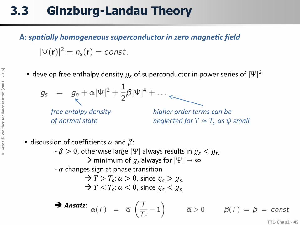
A: spatially homogeneous superconductor in zero magnetic field
• develop free enthalpy density 𝑔𝑠 of superconductor in power series of Ψ 2
free entalpy densityof normal state
higher order terms can beneglected for 𝑇 ≃ 𝑇𝑐 as 𝜓 small
• discussion of coefficients 𝛼 and 𝛽:- 𝛽 > 0, otherwise large |Ψ| always results in 𝑔𝑠 < 𝑔𝑛
minimum of 𝑔𝑠 always for Ψ → ∞- 𝛼 changes sign at phase transition
𝑇 > 𝑇𝑐: 𝛼 > 0, since 𝑔𝑠 > 𝑔𝑛
𝑇 < 𝑇𝑐: 𝛼 < 0, since 𝑔𝑠 < 𝑔𝑛
Ansatz:
Page 46
R. G
ross
© W
alth
er-
Me
ißn
er-
Inst
itu
t (2
00
1 -
20
15
)
TT1-Chap2 - 46
3.3 Ginzburg-Landau Theory
-0.8 -0.4 0.0 0.4 0.8-1
0
1
2
3
4
g s - g
n (
arb
. un
its)
Y (arb. units)
-0.8 -0.4 0.0 0.4 0.8-1
0
1
2
3
4
g s - g
n (
arb
. un
its)
Y (arb. units)
Bcth2 / 2µ0
𝝍𝟎
a < 0T < Tc
a > 0T > Tc
(a) (b)
𝒈𝒔 − 𝒈𝒏 for 𝑻 < 𝑻𝒄 and 𝑻 > 𝑻𝒄
Page 47
R. G
ross
© W
alth
er-
Me
ißn
er-
Inst
itu
t (2
00
1 -
20
15
)
TT1-Chap2 - 47
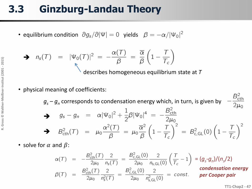
3.3 Ginzburg-Landau Theory
• equilibrium condition yields
describes homogeneous equilibrium state at T
• physical meaning of coefficients:
gs – gn corresponds to condensation energy which, in turn, is given by
• solve for 𝛼 and 𝛽:
= (gs-gn)/(ns/2)
condensation energyper Cooper pair
Page 48
R. G
ross
© W
alth
er-
Me
ißn
er-
Inst
itu
t (2
00
1 -
20
15
)
TT1-Chap2 - 48
3.3 Ginzburg-Landau Theory
Temperature dependence of Bcth:
• GLAG theory prediction:
• experimental observation:
with
reasonable agreement for T close to Tc
GLAG expressions only valid for T close to Tc
Page 49
R. G
ross
© W
alth
er-
Me
ißn
er-
Inst
itu
t (2
00
1 -
20
15
)
TT1-Chap2 - 49
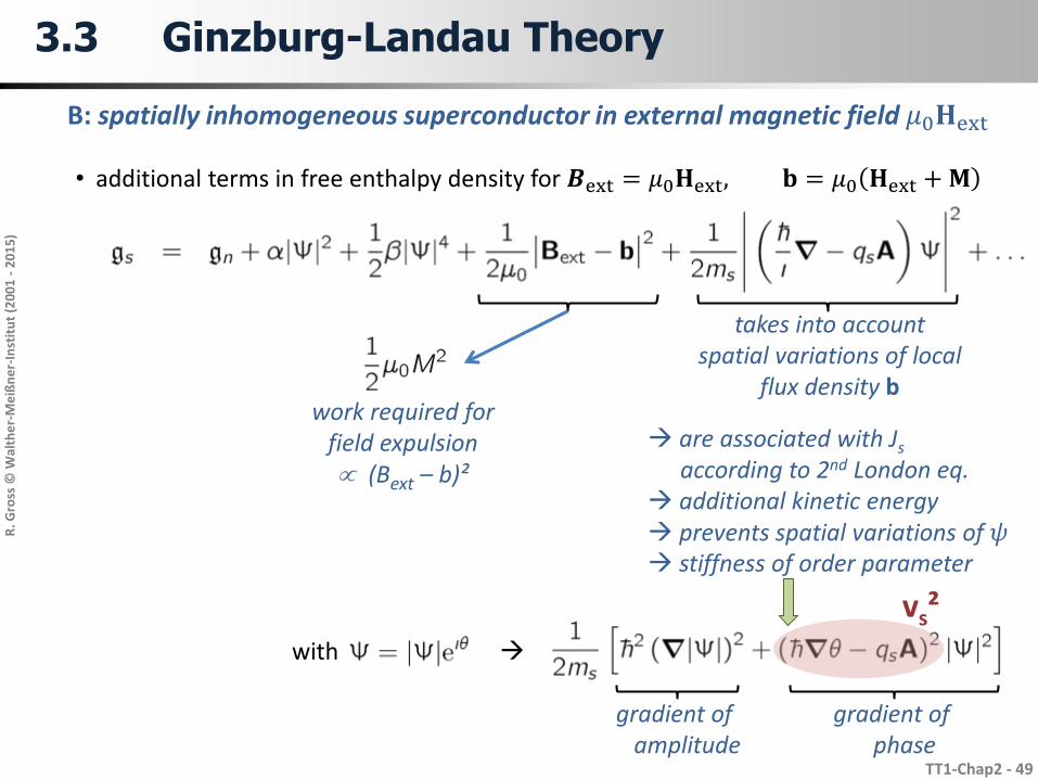
3.3 Ginzburg-Landau Theory
B: spatially inhomogeneous superconductor in external magnetic field 𝜇0𝐇ext
• additional terms in free enthalpy density for 𝑩ext = 𝜇0𝐇ext, 𝐛 = 𝜇0 𝐇ext + 𝐌
takes into accountspatial variations of local
flux density b
are associated with Js
according to 2nd London eq. additional kinetic energy prevents spatial variations of 𝜓 stiffness of order parameter
with
gradient of amplitude
gradient of phase
vs²
work required forfield expulsion (Bext – b)²
Page 50
R. G
ross
© W
alth
er-
Me
ißn
er-
Inst
itu
t (2
00
1 -
20
15
)
TT1-Chap2 - 51
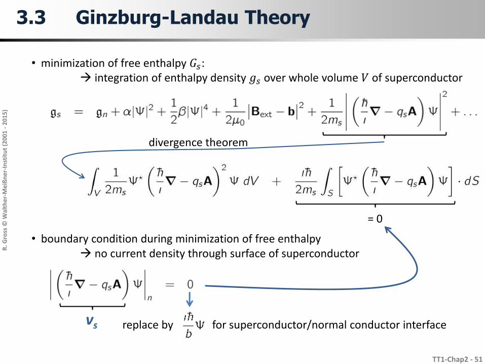
3.3 Ginzburg-Landau Theory
• minimization of free enthalpy 𝐺𝑠: integration of enthalpy density 𝑔𝑠 over whole volume 𝑉 of superconductor
• boundary condition during minimization of free enthalpy no current density through surface of superconductor
replace by for superconductor/normal conductor interfacevs
= 0
divergence theorem
Page 51
R. G
ross
© W
alth
er-
Me
ißn
er-
Inst
itu
t (2
00
1 -
20
15
)
TT1-Chap2 - 54
3.3 Ginzburg-Landau Theory
• minimization of free enthalpy:
• minimization of Gs with respect to variations
= 0, since equation must be satisfied for all
1. Ginzburg-Landau equation
Page 52
R. G
ross
© W
alth
er-
Me
ißn
er-
Inst
itu
t (2
00
1 -
20
15
)
TT1-Chap2 - 55
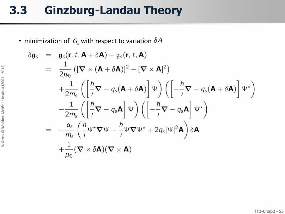
3.3 Ginzburg-Landau Theory
• minimization of Gs with respect to variation
Page 53
R. G
ross
© W
alth
er-
Me
ißn
er-
Inst
itu
t (2
00
1 -
20
15
)
TT1-Chap2 - 56
3.3 Ginzburg-Landau Theory
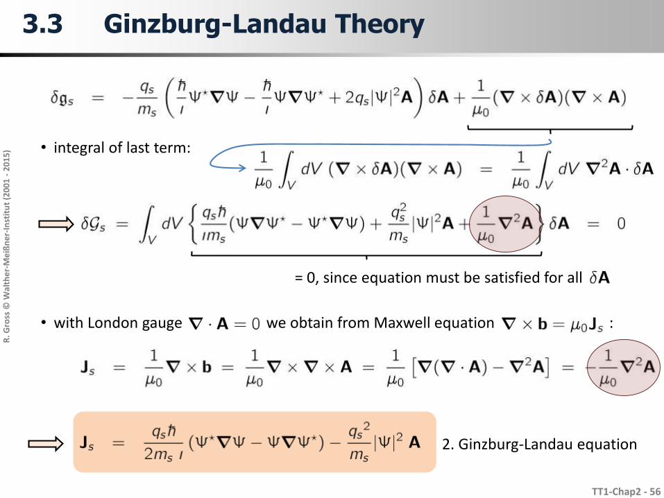
• integral of last term:
• with London gauge we obtain from Maxwell equation :
= 0, since equation must be satisfied for all
2. Ginzburg-Landau equation
Page 54
R. G
ross
© W
alth
er-
Me
ißn
er-
Inst
itu
t (2
00
1 -
20
15
)
TT1-Chap2 - 57
3.3 Ginzburg-Landau Theory
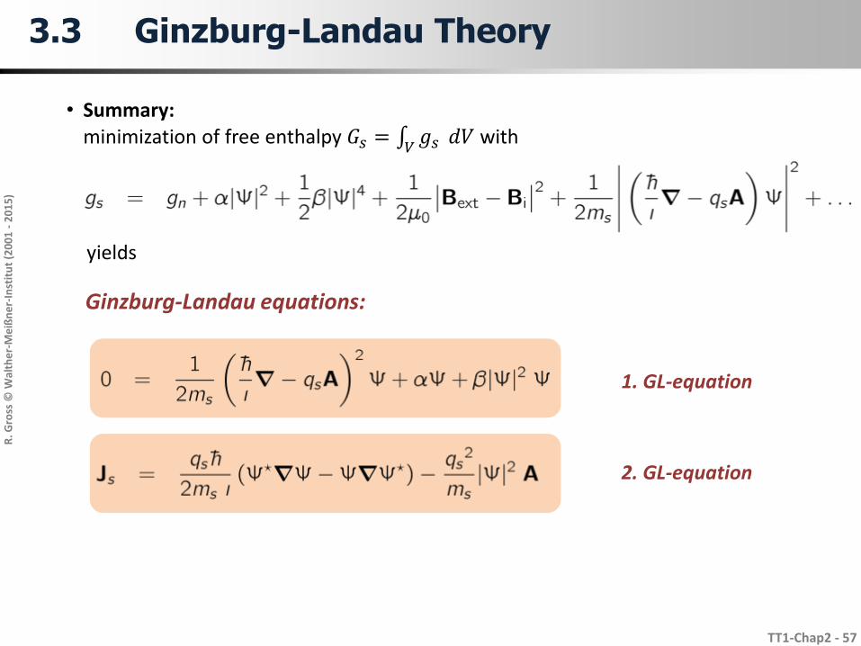
Ginzburg-Landau equations:
1. GL-equation
2. GL-equation
• Summary:minimization of free enthalpy 𝐺𝑠 = 𝑉 𝑔𝑠 𝑑𝑉 with
yields
Page 55
R. G
ross
© W
alth
er-
Me
ißn
er-
Inst
itu
t (2
00
1 -
20
15
)
TT1-Chap2 - 59
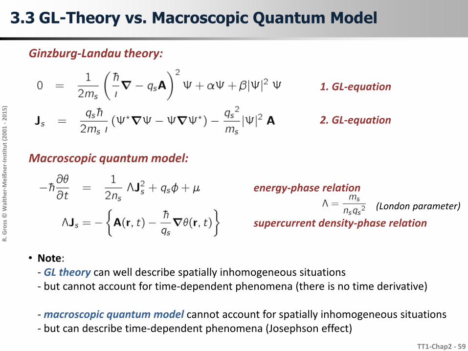
energy-phase relation
supercurrent density-phase relation
(London parameter)
• Note:- GL theory can well describe spatially inhomogeneous situations- but cannot account for time-dependent phenomena (there is no time derivative)
- macroscopic quantum model cannot account for spatially inhomogeneous situations- but can describe time-dependent phenomena (Josephson effect)
Ginzburg-Landau theory:
1. GL-equation
2. GL-equation
Macroscopic quantum model:
3.3 GL-Theory vs. Macroscopic Quantum Model
Page 56
R. G
ross
© W
alth
er-
Me
ißn
er-
Inst
itu
t (2
00
1 -
20
15
)
TT1-Chap2 - 60
3.3 Ginzburg-Landau Theory
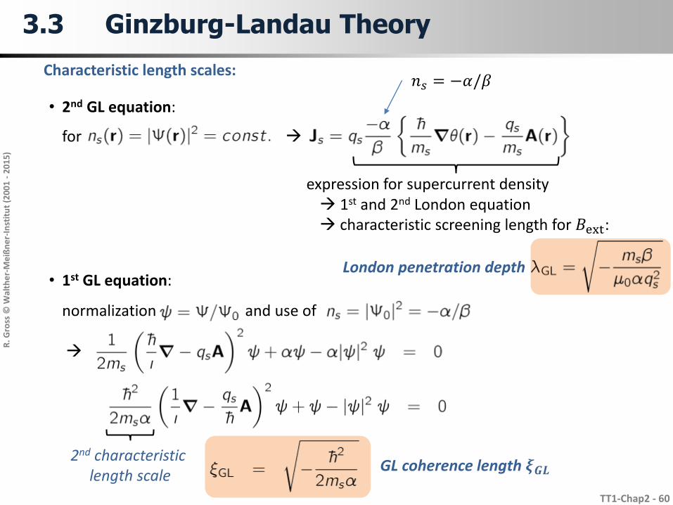
Characteristic length scales:
• 2nd GL equation:
for
expression for supercurrent density 1st and 2nd London equation characteristic screening length for 𝐵ext:
London penetration depth• 1st GL equation:
normalization and use of
2nd characteristic length scale
GL coherence length 𝝃𝑮𝑳
𝑛𝑠 = −𝛼/𝛽
Page 57
R. G
ross
© W
alth
er-
Me
ißn
er-
Inst
itu
t (2
00
1 -
20
15
)
TT1-Chap2 - 61
3.3 Ginzburg-Landau Theory
Temperature dependence of characteristic length scales:
• Ansatz for 𝛼 and 𝛽:
• with and
both length scales diverge for 𝑻 → 𝑻𝒄
experimental T-dependence:
reasonable agreement for T close to Tc
Page 58
R. G
ross
© W
alth
er-
Me
ißn
er-
Inst
itu
t (2
00
1 -
20
15
)
TT1-Chap2 - 62
3.3 Ginzburg-Landau Theory
Ginzburg-Landau parameter:
solve for 𝐵cth
relation between GL and BCS coherence length:
- 𝛼 = condensation energy / (ns /2)
correct BCS result:
- BCS: average condensation energy per electron pair
𝛼/2 corresponds to ≈ −3Δ2(0)/4𝐸𝐹
Page 59
R. G
ross
© W
alth
er-
Me
ißn
er-
Inst
itu
t (2
00
1 -
20
15
)
TT1-Chap2 - 63
3.3 Ginzburg-Landau Theory
Superconductor-normal metal interface:
• solve for x > 0
• assumptions: no magnetic field (𝑨 = 0), 𝜓 𝑥 = 0 = 0
superconductor extends at 𝑥 > 0
• boundary conditions:
and
solution:
Page 60
R. G
ross
© W
alth
er-
Me
ißn
er-
Inst
itu
t (2
00
1 -
20
15
)
TT1-Chap2 - 64
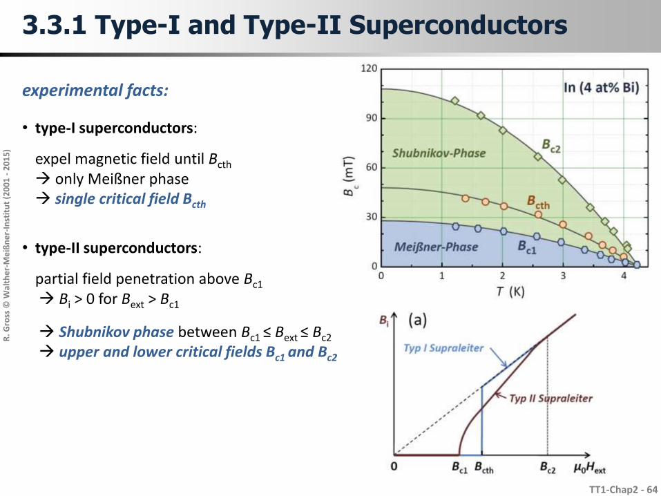
3.3.1 Type-I and Type-II Superconductors
• type-I superconductors:
expel magnetic field until Bcth
only Meißner phase single critical field Bcth
• type-II superconductors:
partial field penetration above Bc1
Bi > 0 for Bext > Bc1
Shubnikov phase between Bc1 ≤ Bext ≤ Bc2
upper and lower critical fields Bc1 and Bc2
experimental facts:
Page 61
R. G
ross
© W
alth
er-
Me
ißn
er-
Inst
itu
t (2
00
1 -
20
15
)
TT1-Chap2 - 65
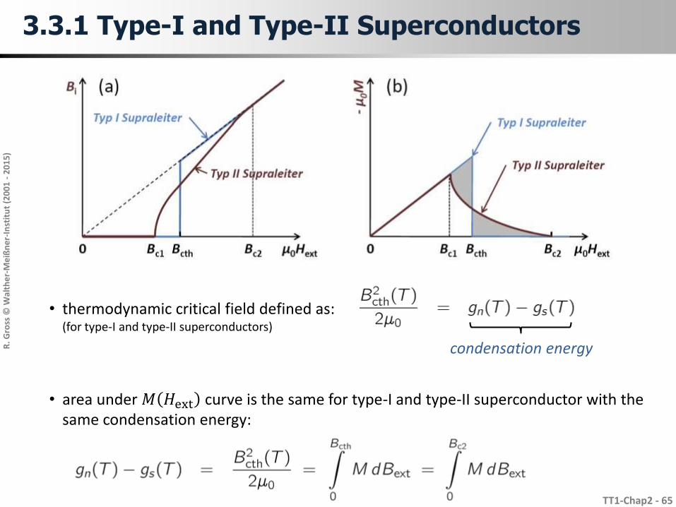
3.3.1 Type-I and Type-II Superconductors
• thermodynamic critical field defined as:(for type-I and type-II superconductors)
• area under 𝑀 𝐻ext curve is the same for type-I and type-II superconductor with the same condensation energy:
condensation energy
Page 62
R. G
ross
© W
alth
er-
Me
ißn
er-
Inst
itu
t (2
00
1 -
20
15
)
TT1-Chap2 - 66
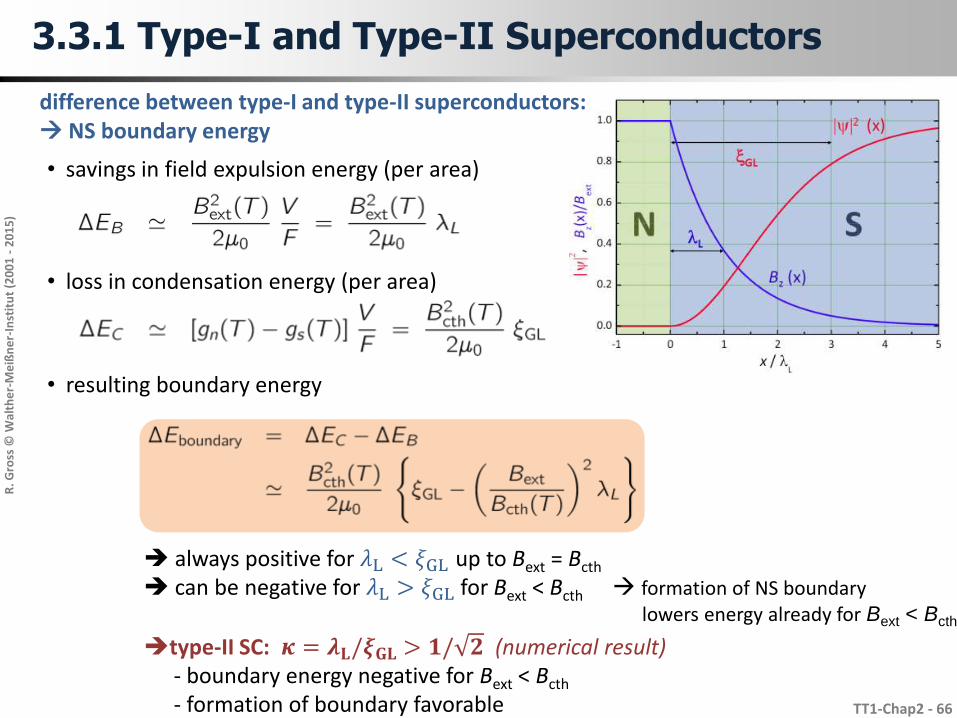
3.3.1 Type-I and Type-II Superconductors
difference between type-I and type-II superconductors: NS boundary energy
• savings in field expulsion energy (per area)
• loss in condensation energy (per area)
• resulting boundary energy
always positive for 𝜆L < 𝜉GL up to Bext = Bcth
can be negative for 𝜆L > 𝜉GL for Bext < Bcth formation of NS boundary lowers energy already for Bext < Bcth
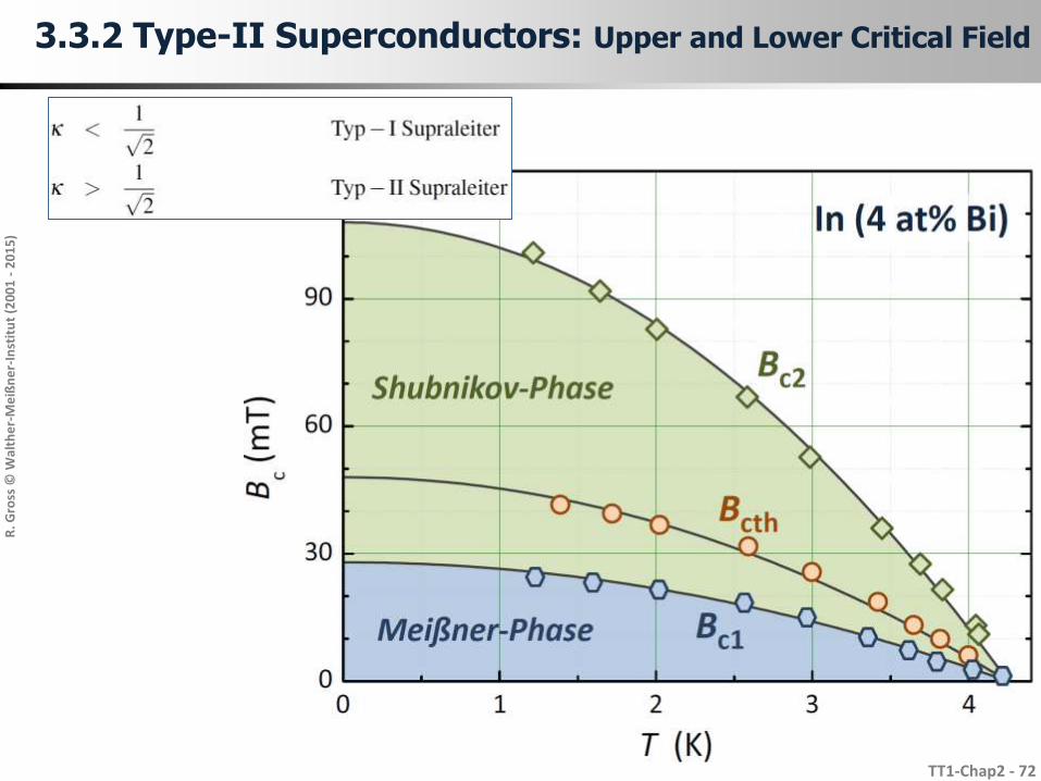
type-II SC: 𝜿 = 𝝀𝐋/𝝃𝐆𝐋 > 𝟏/ 𝟐 (numerical result)- boundary energy negative for Bext < Bcth
- formation of boundary favorable
Page 63
R. G
ross
© W
alth
er-
Me
ißn
er-
Inst
itu
t (2
00
1 -
20
15
)
TT1-Chap2 - 67
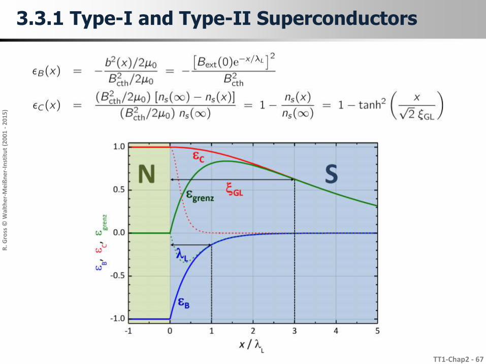
3.3.1 Type-I and Type-II Superconductors
Page 64
R. G
ross
© W
alth
er-
Me
ißn
er-
Inst
itu
t (2
00
1 -
20
15
)
TT1-Chap2 - 68
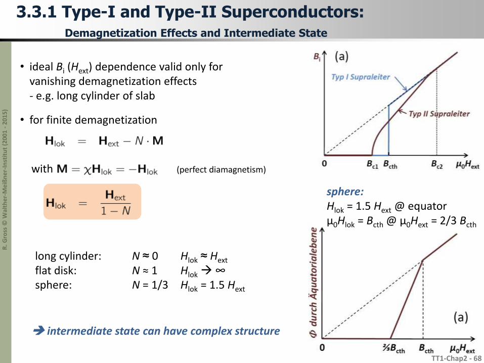
3.3.1 Type-I and Type-II Superconductors: Demagnetization Effects and Intermediate State
• ideal Bi (Hext) dependence valid only forvanishing demagnetization effects- e.g. long cylinder of slab
• for finite demagnetization
with (perfect diamagnetism)
long cylinder: N ≈ 0 Hlok ≈ Hext
flat disk: N ≈ 1 Hlok ∞sphere: N = 1/3 Hlok = 1.5 Hext
sphere:Hlok = 1.5 Hext @ equatorµ0Hlok = Bcth @ µ0Hext = 2/3 Bcth
intermediate state can have complex structure
Page 65
R. G
ross
© W
alth
er-
Me
ißn
er-
Inst
itu
t (2
00
1 -
20
15
)
TT1-Chap2 - 69
3.3.1 Type-I and Type-II Superconductors: Demagnetization Effects and Intermediate State
magneto-optical image
of the intermediate state of In
bright: normal regions
(from Buckel)
Page 66
R. G
ross
© W
alth
er-
Me
ißn
er-
Inst
itu
t (2
00
1 -
20
15
)
TT1-Chap2 - 70
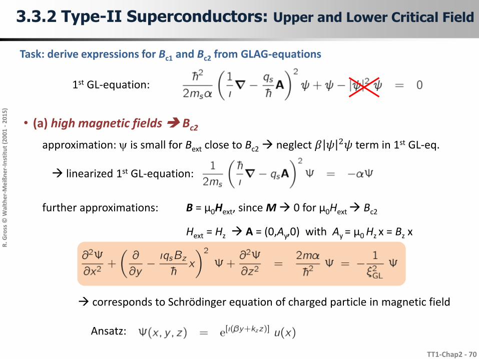
3.3.2 Type-II Superconductors: Upper and Lower Critical Field
Task: derive expressions for Bc1 and Bc2 from GLAG-equations
• (a) high magnetic fields Bc2
approximation: y is small for Bext close to Bc2 neglect 𝛽 𝜓 2𝜓 term in 1st GL-eq.
linearized 1st GL-equation:
further approximations: B = µ0Hext, since M 0 for µ0Hext Bc2
Hext = Hz A = (0,Ay,0) with Ay = µ0 Hz x = Bz x
corresponds to Schrödinger equation of charged particle in magnetic field
Ansatz:
1st GL-equation:
Page 67
R. G
ross
© W
alth
er-
Me
ißn
er-
Inst
itu
t (2
00
1 -
20
15
)
TT1-Chap2 - 71
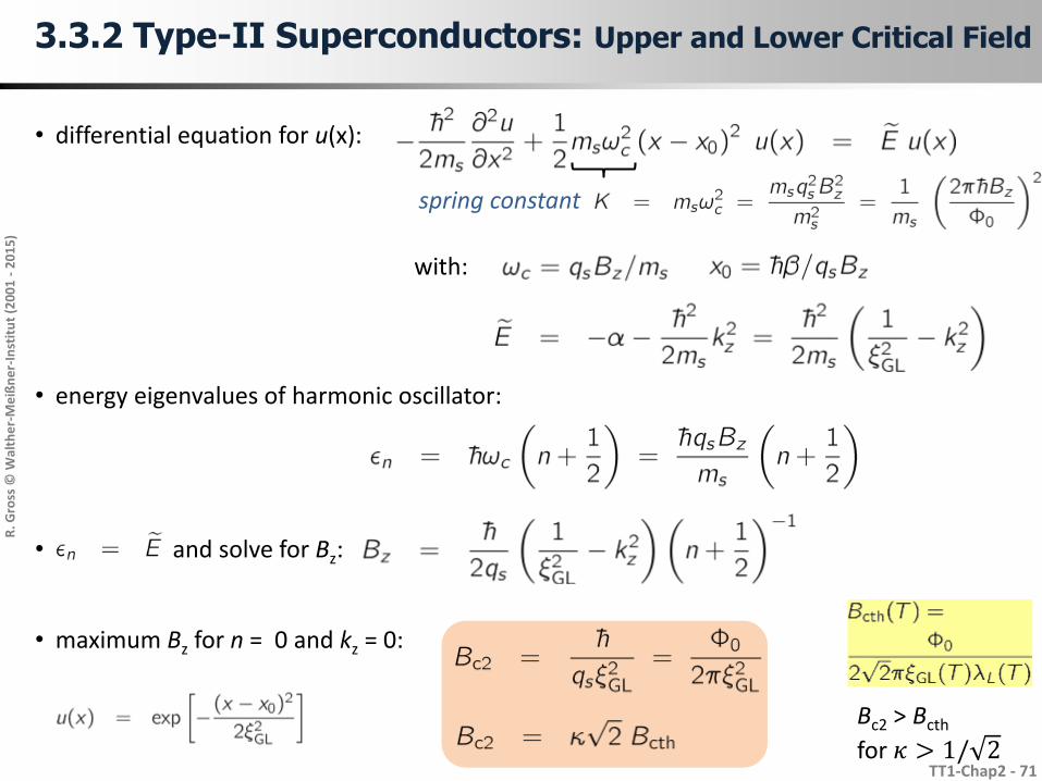
3.3.2 Type-II Superconductors: Upper and Lower Critical Field
• differential equation for u(x):
with:
spring constant
• energy eigenvalues of harmonic oscillator:
• and solve for Bz:
• maximum Bz for n = 0 and kz = 0:
Bc2 > Bcth
for 𝜅 > 1/ 2
Page 68
R. G
ross
© W
alth
er-
Me
ißn
er-
Inst
itu
t (2
00
1 -
20
15
)
TT1-Chap2 - 72
3.3.2 Type-II Superconductors: Upper and Lower Critical Field
Page 69
R. G
ross
© W
alth
er-
Me
ißn
er-
Inst
itu
t (2
00
1 -
20
15
)
TT1-Chap2 - 73
3.3.2 Type-II Superconductors: Upper and Lower Critical Field
𝑩𝒄𝒕𝒉 and 𝝀𝑳 of type-I superconductors
𝑩𝒄𝟐 and 𝝀𝑳 of type-II superconductors
Page 70
R. G
ross
© W
alth
er-
Me
ißn
er-
Inst
itu
t (2
00
1 -
20
15
)
TT1-Chap2 - 74
3.3.2 Type-II Superconductors: Upper and Lower Critical Field
𝑩𝒄𝟐 of type-II superconductors
Page 71
R. G
ross
© W
alth
er-
Me
ißn
er-
Inst
itu
t (2
00
1 -
20
15
)
TT1-Chap2 - 75
3.3.2 Type-II Superconductors: Upper and Lower Critical Field
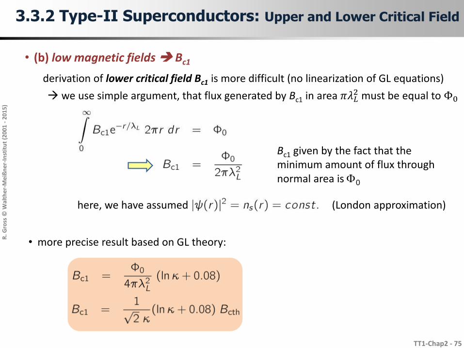
• (b) low magnetic fields Bc1
derivation of lower critical field Bc1 is more difficult (no linearization of GL equations)
• more precise result based on GL theory:
we use simple argument, that flux generated by Bc1 in area 𝜋𝜆𝐿2 must be equal to Φ0
here, we have assumed (London approximation)
Bc1 given by the fact that theminimum amount of flux throughnormal area is F0
Page 72
R. G
ross
© W
alth
er-
Me
ißn
er-
Inst
itu
t (2
00
1 -
20
15
)
TT1-Chap2 - 76
3.3.3 Type-II Superconductors: Shubnikov Phase and
flux Line Lattice
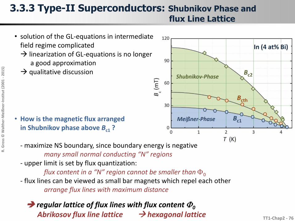
• solution of the GL-equations in intermediate field regime complicated linearization of GL-equations is no longer
a good approximation qualitative discussion
• How is the magnetic flux arranged in Shubnikov phase above Bc1 ?
- maximize NS boundary, since boundary energy is negative many small normal conducting “N” regions
- upper limit is set by flux quantization: flux content in a “N” region cannot be smaller than F0
- flux lines can be viewed as small bar magnets which repel each otherarrange flux lines with maximum distance
regular lattice of flux lines with flux content F0
Abrikosov flux line lattice hexagonal lattice
Page 73
R. G
ross
© W
alth
er-
Me
ißn
er-
Inst
itu
t (2
00
1 -
20
15
)
TT1-Chap2 - 77
3.3.3 Type-II Superconductors: Shubnikov Phase and
flux Line Lattice
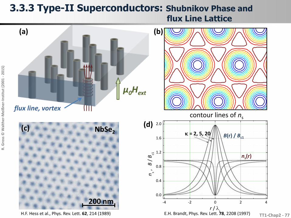
k = 2, 5, 20 B(r) / Bc1
ns(r)
-4 -2 0 2 4
0.0
0.4
0.8
1.2
1.6
2.0
ns ,
B /
Bc1
r / lL
µ0Hext
200 nm
(a)
(c)
(b)
(d)
H.F. Hess et al., Phys. Rev. Lett. 62, 214 (1989) E.H. Brandt, Phys. Rev. Lett. 78, 2208 (1997)
flux line, vortex
NbSe2
contour lines of ns
Page 74
R. G
ross
© W
alth
er-
Me
ißn
er-
Inst
itu
t (2
00
1 -
20
15
)
TT1-Chap2 - 78
3.3.3 Type-II Superconductors: Shubnikov Phase and
flux Line Lattice
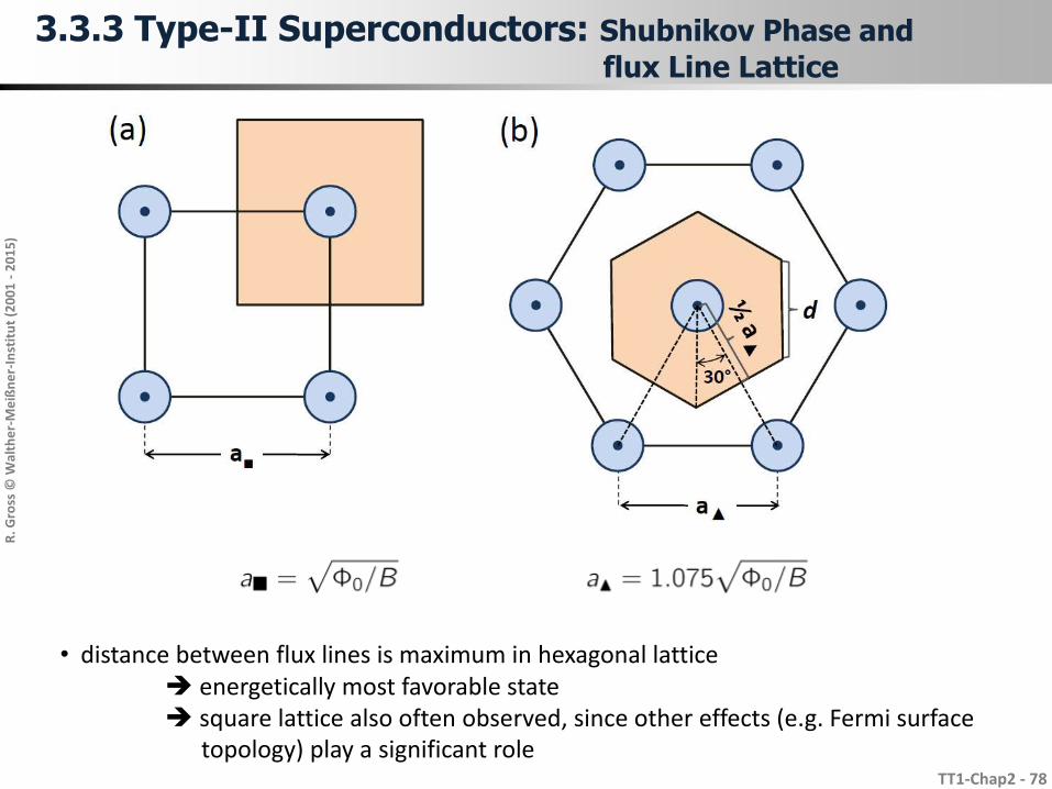
• distance between flux lines is maximum in hexagonal lattice energetically most favorable state square lattice also often observed, since other effects (e.g. Fermi surface
topology) play a significant role
Page 75
R. G
ross
© W
alth
er-
Me
ißn
er-
Inst
itu
t (2
00
1 -
20
15
)
TT1-Chap2 - 79
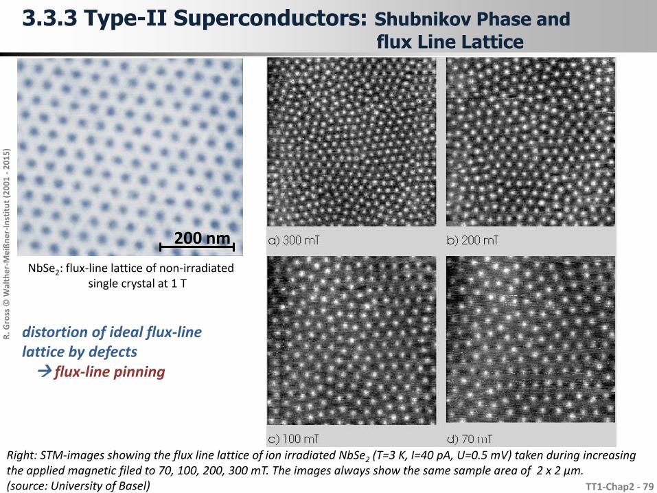
Right: STM-images showing the flux line lattice of ion irradiated NbSe2 (T=3 K, I=40 pA, U=0.5 mV) taken during increasingthe applied magnetic filed to 70, 100, 200, 300 mT. The images always show the same sample area of 2 x 2 µm.(source: University of Basel)
3.3.3 Type-II Superconductors: Shubnikov Phase and
flux Line Lattice
200 nm
NbSe2: flux-line lattice of non-irradiated single crystal at 1 T
distortion of ideal flux-linelattice by defects flux-line pinning
Page 76
R. G
ross
© W
alth
er-
Me
ißn
er-
Inst
itu
t (2
00
1 -
20
15
)
TT1-Chap2 - 80
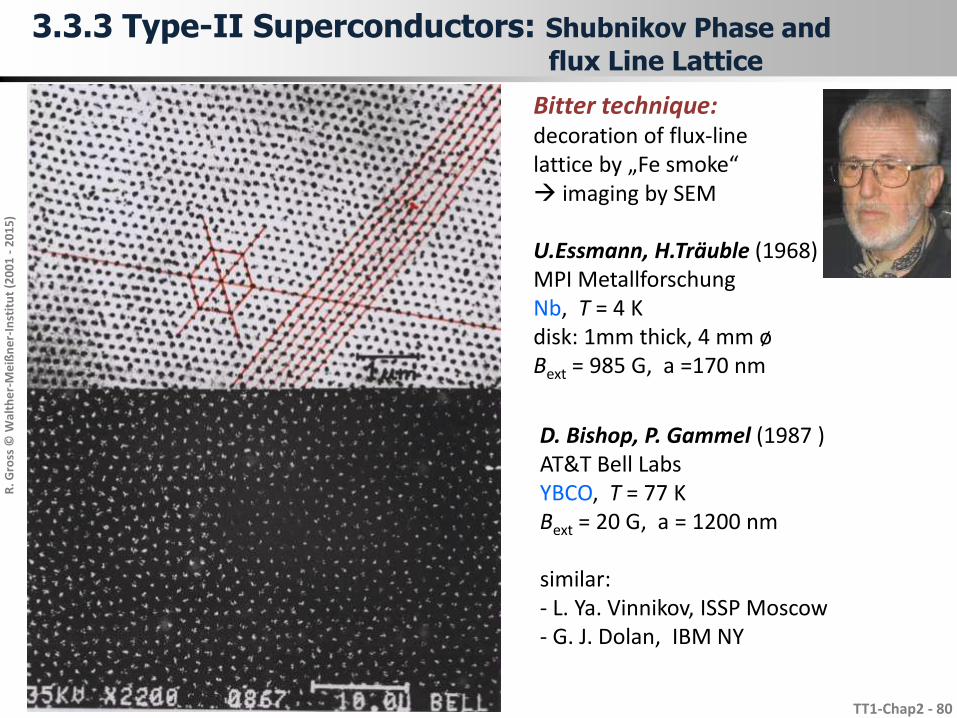
Bitter technique:decoration of flux-linelattice by „Fe smoke“ imaging by SEM
U.Essmann, H.Träuble (1968) MPI MetallforschungNb, T = 4 Kdisk: 1mm thick, 4 mm ø Bext = 985 G, a =170 nm
D. Bishop, P. Gammel (1987 )AT&T Bell Labs YBCO, T = 77 K Bext = 20 G, a = 1200 nm
similar:- L. Ya. Vinnikov, ISSP Moscow- G. J. Dolan, IBM NY
3.3.3 Type-II Superconductors: Shubnikov Phase and
flux Line Lattice
Page 77
R. G
ross
© W
alth
er-
Me
ißn
er-
Inst
itu
t (2
00
1 -
20
15
)
TT1-Chap2 - 82
3.3.4 Type-II Superconductors: Flux Lines
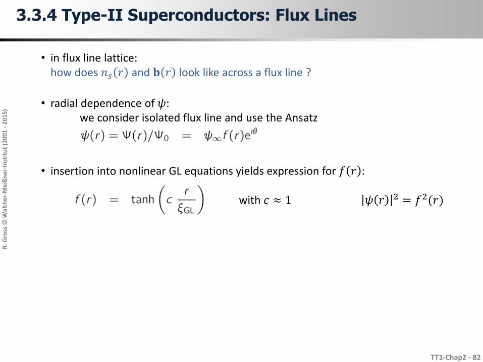
• in flux line lattice:how does 𝑛𝑠 𝑟 and 𝐛 𝑟 look like across a flux line ?
• radial dependence of 𝜓:we consider isolated flux line and use the Ansatz
• insertion into nonlinear GL equations yields expression for 𝑓 𝑟 :
with 𝑐 ≈ 1 𝜓 𝑟 2 = 𝑓2(𝑟)
Page 78
R. G
ross
© W
alth
er-
Me
ißn
er-
Inst
itu
t (2
00
1 -
20
15
)
TT1-Chap2 - 83
3.3.4 Type-II Superconductors: Flux Lines
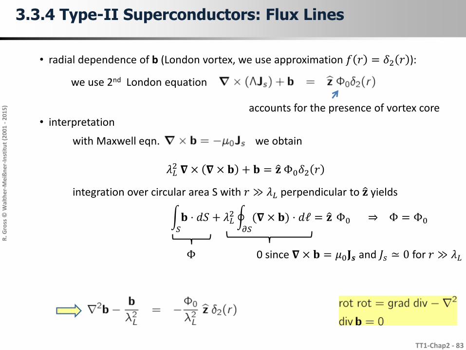
• radial dependence of b (London vortex, we use approximation 𝑓 𝑟 = 𝛿2 𝑟 ):
we use 2nd London equation
accounts for the presence of vortex core• interpretation
with Maxwell eqn. we obtain
𝜆𝐿2 𝛁 × 𝛁 × 𝐛 + 𝐛 = 𝐳 Φ0𝛿2 𝑟
integration over circular area S with 𝑟 ≫ 𝜆𝐿 perpendicular to 𝐳 yields
𝑆
𝐛 ⋅ 𝑑𝑆 + 𝜆𝐿2
𝜕𝑆
(𝛁 × 𝐛) ⋅ 𝑑ℓ = 𝐳 Φ0 ⇒ Φ = Φ0
Φ 0 since 𝛁 × 𝐛 = 𝜇0𝐉𝒔 and 𝐽𝑠 ≃ 0 for 𝑟 ≫ 𝜆𝐿
Page 79
R. G
ross
© W
alth
er-
Me
ißn
er-
Inst
itu
t (2
00
1 -
20
15
)
TT1-Chap2 - 84
3.3.4 Type-II Superconductors: Flux Lines
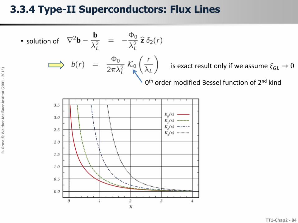
• solution of
0th order modified Bessel function of 2nd kind
is exact result only if we assume 𝜉𝐺𝐿 → 0
Page 80
R. G
ross
© W
alth
er-
Me
ißn
er-
Inst
itu
t (2
00
1 -
20
15
)
TT1-Chap2 - 85
3.3.4 Type-II Superconductors: Flux Lines
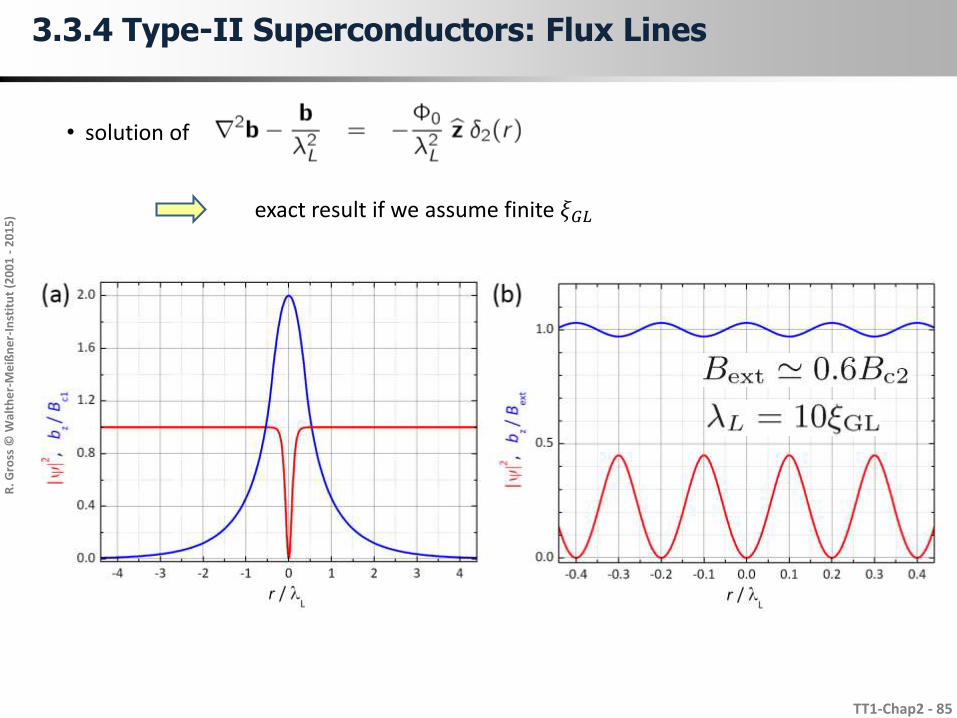
• solution of
exact result if we assume finite 𝜉𝐺𝐿
Page 81
R. G
ross
© W
alth
er-
Me
ißn
er-
Inst
itu
t (2
00
1 -
20
15
)
TT1-Chap2 - 86
3.3 Summary
Literature:• P.G. De Gennes, Superconductivity of Metals and Alloys• M. Tinkham, Introduction to Superconductivity• N.R. Werthamer in Superconductivity, edited by R.D. Parks
The Ginzburg-Landau Theory explains:
• all London results• type-II superconductivity (Shubnikov or vortex state): 𝜉𝐺𝐿 < 𝜆𝐿
• behavior at surface of superconductors and interfaces tonon-superconducting materials
The Ginzburg-Landau Theory does not explain:
• 𝑞𝑠 = − 2𝑒• microscopic origin of superconductivity• not applicable for T << Tc
• non-local effects