Chapter 32

Maxwell’s equations; Magnetism of Matter

Masatsugu Sei Suzuki

Department of Physics, SUNY at Binghamton

(Date: August 15, 2020)

Here we discuss how Maxwell can derive his famous equation.

1. Something is missing; electrodynamics before Maxwell

A statement equivalent to the Coulomb’s law is the differential relation,

0

E (Gauss’ law)

connecting the electric charge density and the electric field E. This holds for moving

charges as well as stationary charges.

0 B (no magnetic monopole)

t

B

E (Faraday’s law)

0 B J (Ampere’s law)

Using the above relations, we calculate

( ) ( ) 0t

E B (OK)

This is consistent. However,

0( ) ( ) B J

The left-hand side of this equation must be zero. But the right-hand side, in general, is not.

For steady state, 0 J is OK. Otherwise, the Ampere’s law cannot be right. This

contradiction shows that the expression for the Ampere’s law cannot be correct for a system

in which the charge density is varying in time.

2. Complete Maxwell’s equation

Maxwell’s equation

The complete Maxwell’s equations are given as follows.

(I)

0

E . (Gauss’ law) (1)

(Flux of E through a closed surface) = -(Charge inside)/0. In dynamics as well as in

static fields, Gauss’ law is always valid.

(II)

t

B

E . (2)

(Line integral of E around a loop) = dt

d (Flux of B through the loop). This is a

Faraday’s law. It is generally true.

(III)

0 B . (3)

(Flux of B through a closed surface) = 0. This equation is the corresponding general

law for magnetic fields. Since there are no magnetic charges, the flux of B through any

closed surface is always zero

(IV)

0 0( )t

E

B J (4)

(Integral of B around a loop) = 0 (current through the loop) + 0 0 (Flux of E through

the loop). This equation has something new. The correct general equation has a new

part that was discovered by Maxwell. 0dt

E

J is called a displacement current.

Conservation of charge

t

J , (equation of continuity) (5)

(Flux of current through a closed surface)=-t

(Charge inside)

Force law

( )q F E v B

From the equation of continuity Eq.(5), we have

0 0( ) ( )t t t

E

J E

or

0( ) 0t

E

J

From Eq.(4)

0 0( ) [ ( )] 0t

E

B J

((Note)) From MIT Physics 8.02: Electricity and Magnetism, Course Notes 2004.

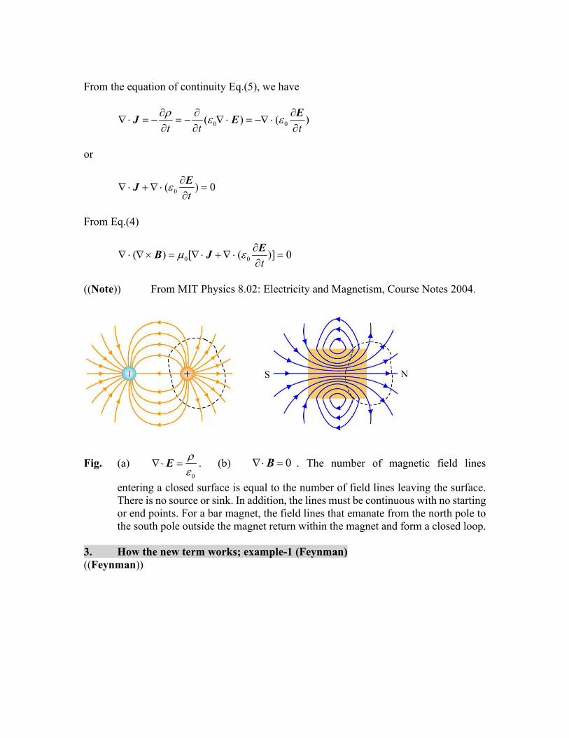
Fig. (a) 0

E . (b) 0 B . The number of magnetic field lines

entering a closed surface is equal to the number of field lines leaving the surface.

There is no source or sink. In addition, the lines must be continuous with no starting

or end points. For a bar magnet, the field lines that emanate from the north pole to

the south pole outside the magnet return within the magnet and form a closed loop.

3. How the new term works; example-1 (Feynman)

((Feynman))

We consider what happens with a spherical symmetric radial distribution of current.

Suppose we imagine a little sphere with radioactive material on it. This radioactive material

is squirting out some charged particles. We could have a current that is everywhere radially

outward.

Let the total charge inside any radius r be Q(r). If the radial current density at the same

radius is J(r), Eq.(5) requires that

2( ) ( ) 4 ( ) ( ) ( )V A V

r d r d r J r r d Q rt t

J J a

2( ) 4 ( )Q r r J rt

We now ask about the magnetic field produced by the current in this situation. Suppose we

draw loop on a sphere of radius r. There is some current through this loop. So we might

expect to find a magnetic field circulating in the direction shown. However, the correct

answer is that there is no magnetic field, B = 0 everywhere. Why is that? This result can

be derived from Eq.(4).

0 0

2 2

0 0

( )

( )

[4 ( ) 4 ( )]

d d

dt

r J r r E rt

B a B s

EJ a

� �

�

Here we note that

2

04

)()(

r

rQrE

Then we have

2

0(4 ( ) ) 0d r J r Qt

B s�

The circulation of B depends not only on the total current through but also on the rate of

change with time of E through it. These two sources cancel and B is always zero. This

implies that there is no magnetic field B everywhere.

4. How the new term works; example of capacitance: Stokes’ theorem

First, we show the definition of the Stokes’ theorem between the surface integral and

the path integral.

Fig. Stokes’ theorem. The surface integral is replaced by the path integral around the

perimeter. ( )S C

d d B a B l� � . The red arrow denotes the direction of da for

each area element. S is the open surface. C is the closed path around the perimeter.

We use the Stokes’ theorem.

02 enc

C

d rB I B l� .

For the surface S1,

encI I .

For the surface S2, the current is the displacement current, but not a current flowing along

the wire.

0enc

dQ d dEI I A A

dt dt dt

,

or

2

d d

S

I I d J a� ,

with

0dt

E

J .

The Ampere’s law can be corrected by Maxwell as

0 0( )t

E

B J .

Fig. Ampere-Maxwell law for the capacitance. S: surface. C: path.

The Stokes’ theorem

0 0( ) enc

S C S

d d d I B a B l J a� � � .

We apply the Stokes’ theorem to the Ampere’s law. We consider the three cases for the

surfaces S1, S2, and S3 for the surface integral, while the path C is the same (fixed).

S1: no capacitance is included

S2: one of the electrodes of the capacitance is included.

S3: both electrodes of the capacitance is included.

For the surfaces S1 or S3, we have

0(2 )B r I , or 0

2

IB

r

,

since

S

d I J a� ,

and

2C

d rB B l� .

For the surface S2, it seems that there is no current enclosed in the surface S3. In order to

get the same result for the magnetic field B, the current I is replaced by the displacement

current.

0d

dQ dEI A I

dt dt .

The current density;

0d

d

I dEJ

A dt .

The ampere’s law:

0 0( )t

E

B J .

where J is the conduction current density and Jd is the displacement current density.

((Note))

E.M. Purcell and D.J. Morin, Electricity and Magnetism 3rd edition (Cambridge 2013).

p.433-434

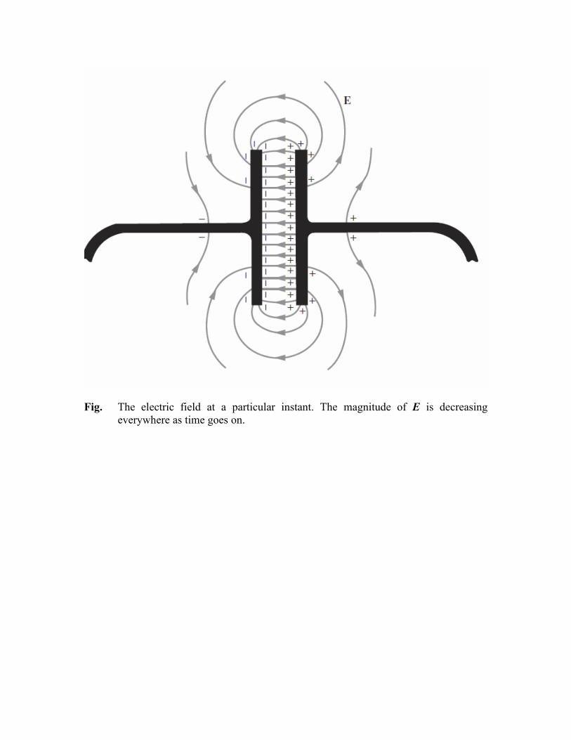
Fig. The electric field at a particular instant. The magnitude of E is decreasing

everywhere as time goes on.

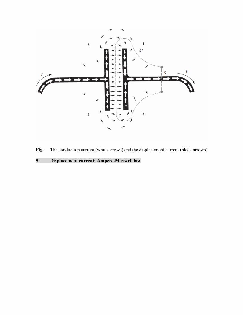
Fig. The conduction current (white arrows) and the displacement current (black arrows)

5. Displacement current: Ampere-Maxwell law

We consider the magnetic field of a wire used to charge a parallel-plate condenser. If

the charge Q on the plate is charging with time, the current in the wires is equal to dQ/dt.

(a) Path 1

Suppose we take a loop 1 which is a circle with radius r.

0 0 0 0( ) ( ) ( )S S

d d d I dt t

E E

B a B s J a a�

If we consider the appropriate plane surface S enclosed by the loop 1, there are no electric

fields on it (assuming the wire to be a very good conductor). The surface integral of

dt

E

a is zero. Then the magnetic field is obtained as

r

IB

2

0

Suppose, however, that we now slowly move the curve downward. We get always

the same result until we draw with the plates of the capacitor. The current I goes to zero.

What happens to the magnetic field?

(b) Path 2

Let’s see what the Maxwell’s equation says for the curve 2, which is a circle of radius

r whose plane passes between the capacitor plates.

0 0

2

S

d rB

dt

B s

E a

�

In other words, the line of integral of B around 2 is equal to the time derivative of the flux

of E through the appropriate plane circular surface S enclosed by the path 2. From the

Gauss’ law, we know that the flux of E through the plane circular surface S is

0S

Qd

E a

Note that the electric field inside the capacitor plate is equal to zero because of metal in

applying the Gauss’ law. Then we have

0 0 0 0 0 0

02 2 2 2S

Q IB d Q

r t r t r t r

E a

So we have the same result for B as described above. It is easy to see that this must always

be so by applying the same arguments to the two circular surfaces S1 and S2 enclosed the

paths 1 and 2, respectively. Through S1 there is the current I, but no electric flux. Through

S2 there is no current, but an electric flux changing at the rate I/0.

The displacement current flows in the separation gap of the capacitance,

0

0

d

d

t

Ei A

t

EJ

6. Magnetism and electrons

6.1. Orbital angular momentum and orbital magnetic moment

If an electron [charge –e (e>0) and mass m] is moving in a circular orbit, there is a

definite ratio between the magnetic moment and the angular momentum. Suppose that L is

the orbital angular momentum and orb is the orbital magnetic moment. The orbital angular

momentum L is given by

ˆmvrz L r p

The direction of L is perpendicular to the plane of the orbit. The orbital magnetic moment

is given by

2ˆ ˆ ˆ2 2

L

ev evrIAz r z z

r

μ ,

where A (= r is the area of the orbit and the current I is given by

r

ev

T

eefI

2 ,

where T (=2r/v) is a period and f (=1/T) is the frequency. So we have the relation between

the orbital angular momentum and the orbital magnetic moment as

( )ˆ

2 2orb

e mvr ez

m m μ L .

The direction of the current is opposite to the direction of velocity of electron because the

charge is negative. The orbital magnetic moment of the electron is antiparallel to the orbital

angular momentum.

Fig. Orbital (circular) motion of electron with mass m and a charge –e. The direction

of orbital angular momentum L is perpendicular to the plane of the motion (x-y

plane). The orbital magnetic moment is antiparallel to the orbital angular

momentum.

6.2 Physical meaning of the expression for the magnetic moment

From the definition of the magnetic moment, a loop (orbital) current I flowing around

a circle with a large radius R, produces a magnetic moment given by

IA ,

where A is the area of the large circle. The magnetic moment can be rewritten as

v

I

Lob

ob

e,m

r

1 2 3( ...)

i

i

i

i

IA

I A A A

IA

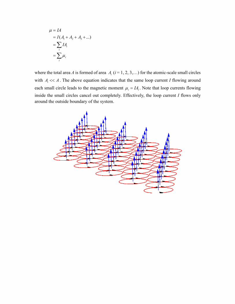
where the total area A is formed of area iA (i = 1, 2, 3,…) for the atomic-scale small circles

with iA A . The above equation indicates that the same loop current I flowing around

each small circle leads to the magnetic moment i iIA . Note that loop currents flowing

inside the small circles cancel out completely. Effectively, the loop current I flows only

around the outside boundary of the system.

Fig. The magnetic moment of the total system is the collection of small magnetic

moments arising from the atomic-scale loop currents I. Evidently, loop currents

flowing inside the system cancel out completely. Only a loop current flowing the

boundary of the system contributes to the resultant magnetic moment. Note that the

direction of each magnetic moment vector is out of page.

6.3 de Broglie relation

Material particles, just like photons, can have a wavelike aspect. The various permitted

energy levels appear as analogues of the normal modes of a vibrating string.

Particle:

E (energy), p (momentum)

Wave:

= 2, k (wave vector)

Relation:

ℏ hE

p kℏ

I

I

I

I

I

I

I

I

I

I

I

I

I

I

I

I

I

I

I

I

I

I

I

I

I

I

I

I

I

I

I

I

I

I

I

I

I

I

I

I

I

I

I

I

I

I

I

I

I

I

I

I

I

I

I

I

I

I

I

I

I

I

I

I

I

I

I

I

I

I

I

I

I

I

I

I

I

I

I

I

I

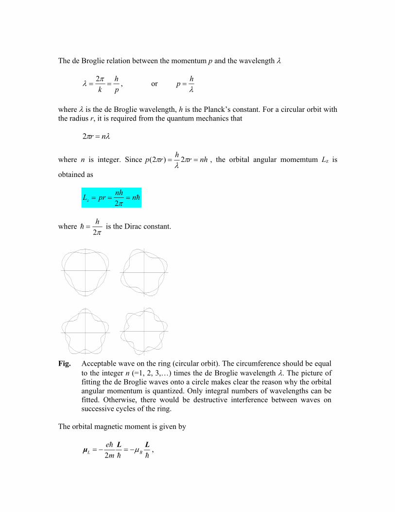
The de Broglie relation between the momentum p and the wavelength

p

h

k

2, or

h

p

where is the de Broglie wavelength, h is the Planck’s constant. For a circular orbit with

the radius r, it is required from the quantum mechanics that

nr 2

where n is integer. Since nhrh

rp

2)2( , the orbital angular momemtum Lz is

obtained as

ℏnnh

prLz 2

where 2

hℏ is the Dirac constant.

Fig. Acceptable wave on the ring (circular orbit). The circumference should be equal

to the integer n (=1, 2, 3,…) times the de Broglie wavelength . The picture of

fitting the de Broglie waves onto a circle makes clear the reason why the orbital

angular momentum is quantized. Only integral numbers of wavelengths can be

fitted. Otherwise, there would be destructive interference between waves on

successive cycles of the ring.

The orbital magnetic moment is given by

2L B

e

m

L Lμ

ℏ

ℏ ℏ,

where B is the Bohr magneton and is

241027400915.9 B J/T (SI units)

or

211027400915.9 B emu (cgs units, emu=erg/Gauss=erg/Oe)

((Note))

J/T = 107 erg/(104 Oe) = 103 emu

J/T2 = 10-1 emu/Oe

The value of the orbital magnetic moment is given by

2L B

en n

m μ

ℏ (n = 1, 2, 3, …)

6.4 Spin angular momentum and spin magnetic moment

The electron also has a spin rotation around its own axis, and as a result of that spin, it

has both a spin angular momentum and a spin magnetic moment. But for reasons that are

purely relativistic quantum-mechanical – there is no classical explanation – the relation

between the spin magnetic moment and the spin angular momentum is different from that

for the orbital motion. The spin magnetic moment is given by

eS B

g

Sμ

ℏ

where ge is the electron g-factor; ge = 2.0023193043622 (NIST). The component of the

spin angular momentum S is measured along the z axis. Then the measured component Sz

can have only the two values given by

ℏ2

1zS ( ; spin up state and ; spin down state).

Then the value of spin magnetic moment is ±B.

6.5 Periodic table of iron group elements

The Pauli principle produces any two electrons being in the same state (i.e., having the

set of (n, l, ml, ms).

For fixed n, l = n-1, n-2, …, 2, 1

ml = l, l-1, …., -l (2l +1).

Therefore there are n2 states for a given n.

There are two values for ms (= ±1/2).

Thus, corresponding to any value of n, there are 2n2 states.

K shell

n l m s ms

1 0 0 1/2 ±1/2 (1s)2

L shell

n l m s ms

2 0 0 1/2 ±1/2 (2s)2

2 1 1,0,-1 1/2 ±1/2 (2p)6

M shell

n l m s ms

3 0 0 1/2 ±1/2 (3s)2

3 1 1,0,-1 1/2 ±1/2 (3p)6

3 2 2,1,0,-1,-2 1/2 ±1/2 (3d)10

N shell

n l m s ms

4 0 0 1/2 ±1/2 (4s)2

4 1 1,0,-1 1/2 ±1/2 (4p)6

4 2 2,1,0,-1,-2 1/2 ±1/2 (4d)10

4 3 3,2,1,0,-1,-2,-3 1/2 ±1/2 (4f)14

(1s)2|(2s)2(2p)6|(3s)2(3p)6(3d)10|(4s)2(4p)6(4d)10(4f)14|(5s)2(5p)6 ((5d)10….

Iron-group elements:

Ti3+, V4+ (1s)2|(2s)2(2p)6|(3s)2(3p)6|(3d)1

V3+ (1s)2|(2s)2(2p)6|(3s)2(3p)6|(3d)2

Cr3+, V2+ (1s)2|(2s)2(2p)6|(3s)2(3p)6|(3d)3

Cr2+, Mn3+ (1s)2|(2s)2(2p)6|(3s)2(3p)6|(3d)4

Mn2+, Fe3+ (1s)2|(2s)2(2p)6|(3s)2(3p)6|(3d)5

Fe2+ (1s)2|(2s)2(2p)6|(3s)2(3p)6|(3d)6

Co2+ (1s)2|(2s)2(2p)6|(3s)2(3p)6|(3d)7

Ni2+ (1s)2|(2s)2(2p)6|(3s)2(3p)6|(3d)8

Cu2+ (1s)2|(2s)2(2p)6|(3s)2(3p)6|(3d)9

Atoms with filled n shells have a total angular momentum and a total spin of zero.

Electrons exterior these closed shells are called valence electrons.

6.6 Magnetic moment of atom

We consider an isolated atom with incomplete shell of electrons. The orbital angular

momentum L and spin angular momentum S are given by

1 2 3 ... L L L L , 1 2 3 ... S S S S (1)

‚l=0

n−1

H2 l+1L êê Simplify

n2

The total angular momentum J is defined by

J L S . (2)

The total magnetic moment is given by

( 2 )B μ L Sℏ

. (3)

The Landé g-factor is defined by

J BJ

g μ J

ℏ, (4)

where

Fig. Basic classical vector model of orbital angular momentum (L), spin angular

momentum (S), orbital magnetic moment (L), and spin magnetic moment (S).

J (= L + S) is the total angular momentum. J is the component of the total

magnetic moment (L + S) along the direction (-J).

Suppose that

a L J L and b S J S

where a and b are constants, and the vectors S and L are perpendicular to J.

Here we have the relation 1 ba , and 0 L S . The values of a and b are determined

as follows.

2a

J L

J,

2b

J S

J. (6)

Here we note that

2 2 2 2 2 2

2 2( )2 2

J L S J L SJ S L S S S L S S , (7)

or 2 2 2 2

[ ( 1) ( 1) ( 1)]2 2

J J L L S S

J L S

J Sℏ

, (8)

using the average in quantum mechanics. The total magnetic moment is

( 2 ) [( 2 ) ( 2 )]B B a b L S

μ L S Jℏ ℏ

. (9)

Thus we have

( 2 ) (1 )B B J BJ

ga b b

μ J J Jℏ ℏ ℏ

, (10)

with

2

3 ( 1) ( 1)1 1

2 2 ( 1)J

S S L Lg b

J J

J S

J. (11)

6.7 Hund’s rule

6.7.1. Electron states in the atom

For a given l, the number m takes 2l +1 values. The number s is restricted to only two

values ±1/2. Hence there are altogether 2(2l+1) different states with the same n and l. There

states are said to be equivalent.

According to Pauli’s principle, there can be only one electron in each such state. Thus

at most 2(2l+1) electrons in an atom can simultaneously have the same n and l.

Hund’s rule is known concerning the relative position of levels with the same configuration

but different L and S.

Hund’first law

(1) The maximum values of the total spin S allowed by the exclusion principle.

Hund’s second law

(2) The maximum values of the total orbital angular momentum L consistent with this

value of S.

Hund’s third law

(i) SLJ for less than half full (spin-orbit interaction, the discussion will be made

later)

(ii) SLJ for more than half full (spin-orbit interaction).

6.6.2. The electron configuration (3d)n (l = 2, n = 1 - 10)

A d shell corresponds to l = 2, with five values of ml. Multiplying this by 2 for the spin

states gives a total of 10. Then the configuration (3d)10 represents a full shell. It is non-

degenerate, and the state is 1S0. This is a general rule for a full shell. It follows because

each of electrons must have a different pair of ml and ms values.

(3d)1: Ti3+, V4+ 2D3/2 (ground state)

L =2, S = 1/2, J = 3/2,

Fig.(a) Hund’s law for the (3d)1 electron configuration.

(3d)2: V3+ 3F2

L =3, S = 1, J = 2,

Fig.(b) Hund’s law for the (3d)2 electron configuration.

(3d)3: Cr3+, V2+ 4F3/2

L =3, S = 3/2, J = 3/2,

Fig.(c) Hund’s law for the (3d)3 electron configuration.

(3d)4: Cr2+, Mn3+ 5D0

L = 2, S = 2, J = 0

Fig.(d) Hund’s law for the (3d)4 electron configuration.

(3d)5: Fe3+, Mn2+ 6S5/2

L = 0, S = 5/2, J = 5/2

Fig.(e) Hund’s law for the (3d)5 electron configuration.

(3d)6: Fe2+ 5D4

L = 2, S = 2, J = 4

Fig.(f) Hund’s law for the (3d)6 electron configuration.

(3d)7: Co2+ 4F9/2

L = 3, S = 3/2, J = 9/2

Fig.1(g) Hund’s law for the (3d)7 electron configuration.

(3d)8: Ni2+ 3F4

L = 3, S = 1, J = 4

Fig.(h) Hund’s law for the (3d)8 electron configuration.

(3d)9: Cu2+ 2D5/2

L = 2, S = 1/2, J = 5/2

Fig.(i) Hund’s law for the (3d)9 electron configuration.

(3d)9

This configuration represents a set of electrons one short of a full shell. Since a full shell

has zero angular momentum (both orbital and spin), it follows that if one electron is

removed from a full shell, the spin angular momentum of the remainder are minus those of

the one that was removed. So the L, S, and J values of remainder are the same as if there

were only one electron in the shell.

(3d)10

A d shell corresponds to l = 2, with five values of ml. Multiplying this by two for the spin

states gives 10. Thus the configuration (3d)10 represents a full shell. L = 0. S = 0. J = 0.

7. Definition of the magnetization

We define the magnetization M of a material as the net magnetic moment per unit

volume. If there are n atoms per unit volume and their average magnetic moment is , then

M can be written as

nM μ

The total magnetic moment of the system is tot. The volume of the system is V. Then the

magnetization of the system is defined by

tot

V

μM

The unit of M is J/(T m3) in SI units and emu/cm3 in cgs units.

8. Paramagnetism: classical theory

We assume that a magnetic dipole moment of each molecule in the presence of a

magnetic field B. The potential energy is given by

cosU B μ B

where N is the number of magnetic dipole moments per unit volume and is the angle

between and B. Then the magnetization M is given by

cosNM

where

0

cos0

cos

)sin2(

)sin2(coscos

cos

de

de

de

de

Tk

B

Tk

B

Tk

U

Tk

U

B

B

B

B

and kB is the Boltzmann constant. For simplicity we put

Tk

Bx

B

and coss .

Then we have

)(1

cothcos1

1

1

1 xLx

x

dse

sdse

sx

sx

where L(x) is the Langevin function. For x<<1, the Langevin function is approximated as

3.....

453)(

3 xxxxL

and the derivative dL(x)/dx at x = 0 is equal to 1/3. Using this we have

Tk

BNxNxLNM

B33)(

2

9. Magnetization for the spin 1/2 system (quantum mechanics)

We discuss the magnetization for spin 1/2. The system consists of many spins (the

number N per unit volume). There is no interaction between any two spins. The magnetic

moment of spin (S = 1/2) is given by

zzBz S ˆ/ˆ2ˆ ℏ ,

where z is a Pauli spin operator along the z axis. Then the Zeeman energy is described

by

BBH zz ˆˆˆ , (1)

in the presence of a magnetic field B along the z axis.

Fig. Zeeman splitting of the degenerate state under the application of magnetic field B.

The doublet state (degenerate) is split into two states:

1. lower energy level (-BB): state ; B (magnetic moment)

2. upper energy state (BB): state ; -B (magnetic moment)

The probability of finding the system in the lower state

xx

x

ee

e

N

N

1

where x = /(kBT). The probability of finding the system in the upper state is

xx

x

ee

e

N

N

2

The total magnetization M is

xNee

eeNNNM

xx

xx

tanh)( 21

. (2)

(a) For x>>1, tanhx ≈ 1,

M = Msat = N.

(b) For x<<1, tanhx ≈ x.

BTk

N

Tk

BNM

BB

2

. (3)

for S = 1/2.

((Curie law))

In 1895, Pierre Curie discovered this experimentally. The magnetization is directly

proportional to the magnitude of the external magnetic field B and inversely proportional

to the temperature T in K.

T

C

B

M

where C is called the Curie constant.

10. Ferromagnetism

10.1 Ferromagnetic order

A ferromagnet has a spontaneous magnetization – a magnetization even in zero applied

magnetic field. The existence of a spontaneous magnetization suggests that the magnetic

moments are arranged in a regular manner. Consider a paramagnet with ions having

magnetic moments. Given an internal interaction tending to line up the magnetic moments

parallel to each other, we shall have a ferromagnet. Let us postulate such an interaction and

call it the exchange field. We treat the exchange field as equivalent to a magnetic field BE.

The magnitude of the exchange field may be as high as 103 T. This field BE is proportional

to the magnetization M, and is described by

MBE 0 (mean field)

Fig. Ferromagnetic spin order

10.2 Curie temperature

I

((Note)) See Chapter 29S for the detail

Fig. The field at any point A in a magnetic system can be considered as the sum of the

field in a spherical hole plus the field due to a spherical plug.

For the spherical hole, the magnetic field is given by

0

2

3plug B M

0

0 0

0

2

3

2( )

3

1( )

3

hole

B B M

H M M

H M

In Chapter 29, we show that the magnetic field in the hole (sphere) is given by

MBB ahole 0

where Ba (= 0H) is the external magnetic field, and is dependent on the shape of the hole

and = 1/3 for sphere. For a spin S = 1/2, it is known that the magnetization M is given by

)tanh(xyM

M

s

(a)

where Ms (= N) is the saturation magnetization. For x<<1, tanh(x) is approximated as

3)tanh(

3xxx .

The variable x is expressed by

yTk

N

Tk

B

MM

M

TkTk

B

MBTkTk

Bx

BB

a

sat

satBB

a

a

BB

hole

2

0

0

0 )(

where Msat (= N) is the saturation magnetization. This equation can be rewritten as

)(2

0 Tk

Bx

N

Tky

B

aB

. (b)

For any given value of Ba, this is a straight-line relationship between y and x. The x intercept

is at Tk

Bx

B

a and the slope is

2

0 N

TkB . For any particular Ba, we would have a line like

the one denoted by (b). The intersection of curves (a) and (b) gives us the solution for

M/Msat.

We now look at how the solutions will go for various circumstances. We assume that

Ba = 0.

xT

Ty

xy

c

)tanh(

where the characteristic temperature Tc is called a Curie temperature, and is given by

B

ck

NT

2

0

The slope of the line (b) is proportional to T. When the slope is larger than 1, there is no

solution for finite value of M. For T>Tc, we have a solution M/Msat = 0 (paramagnetic phase).

On the other hand, for T<Tc, we have a solution for the finite value of M/Msat (ferromagnetic

phase). Then the magnetic material should magnetize itself spontaneously below Tc.

10.3 Spontaneous magnetization M

When Ba = 0. y is given by

0.0 0.5 1.0 1.5 2.0x0.0

0.2

0.4

0.6

0.8

1.0tanhHxL

txxT

Ty

c

,

with t = T/Tc. The reduced temperature (t) dependence of the spontaneous magnetization is

a solution of xT

Ty

c

and )tanh(xy .

Fig. Spontaneous magnetization y as a function of t. The value of y is obtained from the

equation y = tanh(y/t). t = T/Tc. y = 1 at t = 0.

10.4. Magnetic susceptibility of ferromagnetism

We now consider the magnetic susceptibility. The straight line is described by

)(Tk

Bx

T

Ty

B

a

c

For x<<1, y = x. Then we have

0.2 0.4 0.6 0.8 1t

0.2

0.4

0.6

0.8

1

y

c

B

a

cB

a

c

B

a

c

TT

k

B

x

Tk

B

T

Tx

xTk

Bx

T

T

)1(

)(

Since y = x, we have

cBa TTk

N

B

M

12

The susceptibility diverges as T approaches Tc from the high temperature side.

Fig. The reciprocal susceptibility as a function of T for stage-2 CrCl3 GIC. B//c (parallel

to the c axis). B = 1 kOe. The straight line denotes the Curie-Weiss law.

0

50

100

150

200

250

300

0 50 100 150 200 250 300

stage-2 CrCl 3 GIC

T(K)

H = 1 kOe

H // c

(b)

11. A brief history on the modern magnetism

Magnetism is inseparable from quantum mechanics. A classical system in thermal

equilibrium can display no magnetic moment, even in a magnetic field (Kittel). The

magnetism is essentially the quantum phenomenon and is a property, reflecting the feature

of quantum mechanics. In his talk titled the quantum mechanics, key to understanding

magnetism (the Nobel lecture, December 8, 1977), Van Vleck pointed out that modern

theories of magnetism have roots in two distinct traditions of theoretical developments.

The first outstanding early attempt to understand magnetism at the atomic level was

provided by the semi-empirical theories of Langevin and Weiss. These theories were able

to explain experimental results on the magnetic properties of materials. Langevin assumed

that an atomic or molecular magnet carries a permanent magnetic moment. He was

quantizing the system without realizing it. If one applies classical dynamics and statistical

mechanics consistently, one finds that the diamagnetic and paramagnetic contributions to

the magnetic susceptibility exactly cancel. Thus there should be no magnetism. The break-

through in understanding of magnetic phenomena at the atomic level occurred in 1913,

when Niels Bohr introduced the significant concept of the quantization of the orbital

angular momentum, as a part of his remarkable theory of the hydrogen spectrum. The

quantization of electron orbits implied the existence of an elementary magnetic moment,

the Bohr magneton. In 1922, Stern and Gerlach experimentally verified the quantized

orbital angular momentum and hence the orbital magnetic moment.

The advent of quantum mechanics in 1926 furnished at last the key to the quantitative

understanding of magnetism, (i) the discovery of the matrix form of quantum mechanics

by Heisenberg and Born, (ii) the alternative but equivalent wave mechanical form by de

Broglie and Schrödinger, and (iii) the introduction of electron spin by Uhlenbeck and

Goulsmit. A quantum mechanics without spin and the Pauli’s exclusion principle would

not have been able to understand even the structure of the periodic table or most magnetic

phenomena. Originally spin was a sort of the appendage to the mathematical framework,

but in 1928, Dirac synthesized everything in his remarkable four first order simultaneous

equations which is relativistically invariant under the Lorentz transformation. The electron

spin and the factor of two came naturally out of the calculation. In 1928, Heisenberg has

shown how the previously obscure Weiss molecular field could be attributed to a quantum

mechanical exchange effect, arising from the Pauli’s exclusion principle that no two

electrons occupy the same state. The forces of interaction between neighboring atoms give

rise to an exchange coupling between unpaired spinning electron. This leads to a scalar

isotropic interaction of two spins with an exchange interaction constant.

12. Magnetization of magnetic systems (summary)

In paramagnetic and diamagnetic materials, the magnetization is maintained by the

field. When the field B is removed, the magnetization M disappears. In Fact, for most

substances, the magnetization is proportional to the field, provided the field is not too great.

For notational consistency with the electrical case, one should express the proportionality

thus:

0

1m

M B (1)

But custom dictates that it be written in terms of H instead of B

mM H (2)

where m is called the magnetic susceptibility. Here we use the notation (1) instead of (2),

since the expression of H is not used in the standard textbook of general physics. Anyway,

we are interested in the magnetization as a function of external magnetic field and

temperature

Experimentally, one can measure the magnetization of samples using the SQUID

(superconducting quantum interference device). Here we discuss the magnetization of three

kinds of systems, paramagnetism, diamagnetism, and ferromagnet. The magnetization is

the magnetic moment per unit volume. The magnetization M for the paramagnetic and

diamagnetic systems can be expressed by

0 0 ( ) mM M B B

where the proportionality constant m is dimensionless number called the magnetic

susceptibility. B is the internal magnetic field. For diamagnetic materials, m is a small

negative constant independent of temperature. For paramagnetic materials, m is positive

and can be expressed by the Curie law.

0 0 0

CM B B

T ,

where T is the temperature and C is the Curie constant and B is equal to the external

magnetic field B0. The Curie law arises from

00 tanh( )

B

BM n

k T

,

for the two-level energy states of spin up and spin down, where n is the number density of

magnetic atoms with magnetic moment . In the high temperature range, we get

0 0tanh( )B B

B B

k T k T

,

leading to

2

00 0

B

n B CM B

k T T

. (Curie law)

with the Curie constant

2

B

nC

k

.

For the ferromagnet, the internal magnetic field B can be expressed by

0 ( )B B M B ,

where is constant and the second term is the mean field arising from the interaction with

the neighboring magnetic moments. We note that the magnetization M is a function of B,

0 0 0( ) ( )C C

M M B B B MT T

,

or

0 0 0

0

c

C CM B B

C T TT

.

Note that Tc is the Curie temperature and is defined by

2

0 0

c

B

C nT

k

.

For cT T , the system is in the ferromagnetic state where all the direction of spins.

Suppose that there is no external magnetic field. it is expected that the spontaneous

magnetization appears below Tc,

0 tanh( )B

MM n

k T

,

or

0 0tanh( )cM M T

n n T

.

We use the parameters y and x as

0My

n

, c

Tx

T .

the above equation can be rewritten as

tanh( )y

yx

.

We make a plot of y vs x using the Mathematica.

Fig. Spontaneous magnetization appears below the Curie temperature.

REFERENCES

D.J. Griffiths, Introduction to Electrodynamics, 2rd edition (Prentice Hall, 1981).

The magnetic susceptibility of typical materials

((Example))

Graphite diamagnetism

levitation experiments

https://www.youtube.com/watch?v=rjBczjGQsdc

Bismuth diamagnetism

https://www.youtube.com/watch?v=A5pZZJ23rDM

Oxygen paramagnetism

https://www.youtube.com/watch?v=Lt4P6ctf06Q

13. Typical problems

13.1 Problem 32-3

A Gaussian surface in the shape of a right circular cylinder with end caps has a radius of

12.0 cm and a length of 80.00 cm. Through one end there is an inward magnetic flux of

25.0 Wb. At the other end there is a uniform magnetic field of 1.60 mT, normal to the

surface and directed outward. What are the (a) magnitude and (b) direction (inward or

outward) of the net magnetic flux through the curved surface?

((Solution))

Gauss’ law for B

0totald d B B a� �

B = 1.60 mT (top surface)

r = 0.12 m

bottom = -25.0 mWb (bottom surface, the magnetic flux going inward)

L = 0.8 m

The total magnetic flux passing through a closed surface should be zero.

0 sidebottomtoptotal

where

Wb

RB

bottomr

top

0.25

)( 2

00.25)( 2 sidetotal WbRB

or

WbWbRBside

52 1074.40.25)(

The magnetic flux passing the side surface goes inward.

13.2 Problem 32-20

A capacitor with parallel circular plates of radius R = 1.20 cm is discharging via a current

of 12.0 A. Consider a loop of radius R/3 that is centered on the central axis between the

plates. (a) How much displacement current is encircled by the loop? The maximum induced

magnetic field has a magnitude of 12.0 mT. At what radius (b) inside and (c) outside the

capacitor gap is the magnitude of the induced magnetic field 3.00 mT?

((Solution))

R = 1.20 cm

i = 12.0 A

(a) AR

riid 333.1

2

2

(b) and (c)

For r<R

2

0 2

2

0 2

2

0 0

2 2

(2 )

2 2

rd i

R

rB r i

R

i r iB r

r R R

B l�

For r>R

0

0

0

(2 )

2

d i

B r i

iB

r

B l�

The maximum of B occurs at r =R.

R

iB

2

0max

Suppose that Bmax = 12 mT. Then we have

R

rBB max for r<R

r

RBB max for r>R

where R = 1.20 cm. We make a plot of B (mT) as a function of r (cm).

1 2 3 4 5 6rHcmL

2

4

6

8

10

12

BHmTL

When B = 3 mT,

r = 0.3 cm or r = 4.8 cm

______________________________________________________________________

13.3 Problem 32-51

A Rowland ring is formed of ferromagnetic material. It is circular in cross section, with

an inner radius of 5.0 cm and an outer radius of 6.0 cm, and is wound with 400 turns of

wire, (a) what current must be set up in the windings to attain a toroidal field of magnitude

B0 = 0.2 mT? (b) A secondary coil wound around the toroid has 50 turns and resistance 8.0

. If, for this value of B0, we have BM = 800 B0, how much charge moves through the

secondary coil when the current in the toroid windings is turned on?

((My solution))

((Solution)) from the text book (Halliday and Resnick)

Np = 400 turns, Ravg = 5.5 cm (in average) = 0.055 m.

Area of circular cross section; A = r2. r = 0.005 m.

Ns = 50. Rs = 8.0

The magnetization of a ferromagnetic material such as iron can be studied with an

arrangement called a Rowland ring. The material is formed into a thin toroidal core of

circular cross section. A primary coil P having n turns per unit length is wrapped around

the core and carries current iP. (The coil is essentially a long solenoid bent into a circle). If

the iron core were not present, the magnitude of the magnetic field inside the coil would

be,

avg

p

pppR

NiinB

2000

p

avg

pN

RBi

0

0

2

= 0.1375 A

However, with the iron core present, the magnetic field B inside the coil is greater than B0,

usually by a large amount. We can write the magnitude of this field as

00 801BBBB M

where BM (= 800 B0) is the magnitude of the magnetic field contributed by the iron core.

This contribution results from the alignment of the atomic dipole moments within the iron,

due to exchange coupling and to the applied magnetic field B0, and is proportional to the

magnetization M of the iron. That is, the contribution BM is proportional to the magnetic

dipole moment per unit volume of the iron.

To determine BM we use a secondary coil S to measure B. The voltage generated across

the secondary coil is given by

dt

dqRiR

dt

dNV s

sssss

or

)( 0 M

s

s

s

ss BBA

R

N

R

Nq = 7.864 x 10-5 C

where

MBBA 0 = 1.258 x 10-5 Wb, 2rA

Note: this method is very familiar to the experimentalists as a principle of the ballistic

galvanometer.

________________________________________________________________________

APPENDIX-1 Core diamagnetism

We consider the diamagnetism from the classical point of view. Suppose that we slowly

turn on the magnetic field. As the magnetic field changes an electric field is generated by

magnetic induction, from the Faraday’s law,

Bd d dt t

B

E a E s a�

or

dt

dBr

trE B

2

02

or

dt

dBr

dt

dB

r

rE

22

0

0

2

0

The induced electric field acting on an electron in the atom produces a torque equal to

2

00 0

ˆ ˆˆ ˆ ˆ( ) ( ) ( )2

d er dBr r e E er E r z

dt dt

Lτ r F

Integrating with respect to time t from zero field, we have

Ber

Lz2

2

The magnetic moment is

][442

222

2

0

2

yxm

Ber

m

BeL

m

ezz

The minus sign means that the added magnetic moment is opposite to the magnetic field.

Here we note that r0 is a radius from an axis through the atom parallel to B. So if B is along

the z axis, r02 = 22 yx . If we consider spherically symmetric atoms, the average of

22 yx is (2/3) of the average of the square of the true radial distance from the center point

of the atom. Then we have

avavz r

m

Ber

m

Be 22

22

6)

3

2(

4

When NA is the Avogadro number and each atom has z electrons, the magnetic

susceptibility is given by

avgavg

AzA rzrm

zeN

B

zN 21522

1082834.26

)(

J/T2

where r is in the units of m. Note that the unit of in the CGS unit is emu/Oe = (emu/Oe2).

The unit of in the SI units is J/T2 = (1/10) emu/Oe.

The sign of is negative, which leads to the diamagnetism of matter. The graphite and

bismuth has a large diamagnetic susceptibility.

((Mathematica))

((Note))

((Another method))

dt

dBr

dt

dB

r

rE

22

0

0

2

0

The force F is related to E as

dt

dB

m

er

dt

dv

dt

dBer

dt

dBreeE

dt

dvmF

2

2)

2(

0

00

or

Bm

erv

2

0

Since

2

0 0 0 0ˆ ˆ ˆ2 2 2 4

L

er er er erv z B z B z

m m

μ

________________________________________________________________________

APPENDIX-2 Maxwell’s equation in the matter

2.1 Maxwell’s equations

The equations governing electromagnetic phenomena are the Maxwell’s equations,

Maxwell’s equation (in general)

0

0 0

0

( )

t

t

E

B

BE

EB J

B: magnetic field

E: electric field

H: (here we call H field)

D: electric displacement vector

0 permittivity of free space

0 permeability of free space

: charge density

J current density

0 ( ) B M H ,

0 D E P

f D

ft

H D J

where

00

1

c

(a) Electric charge

f b f P

where f is the free charge density.

(b) Current density

f b M ft

P

J J J J J M

P: electric polarization vector,

JP: polarization current density

M: magnetization vector

JM: magnetization current density

b

b

bp

p

t

t

P

P n

J

PJ

M J M

2.2 Gauss; law, Ampere’s law

(a) Gauss’s law

0 0

1( )f

E P

or

0( ) ,f E P

or

f D

where

0 D E P (electric displacement)

(b) Ampere’s law

0 0 0 ( )ft t

E P

B J M

or

0 0 0( ) [ ( ) ]ft

B M E P J

Here we define

0 ( ) B M H , and 0 D E P

Then we have

ft

H D J

2.3 Boundary conditions

(a) f D

1 2( ) fa a D D n or 1 2( ) f D D n

where n is the unit vector perpendicular to the boundary surface (normal component).

fDD 21 (normal component)

(b) 0 B

1 2( ) 0a B B n or 1 2( ) 0 B B n

where n is the unit vector perpendicular to the boundary surface (normal component).

021 BB (normal component).

(c) t

B

E

d d d dt t

B

E a E l a B a� � � � (Stokes theorem)

/ / / /

1 2( ) 'E E l t lt

B n

or

/ / / /

1 2( ) ' 0E E tt

B n , when 0t

or

//

2

//

1 EE (tangential component).

(d) ft

H D J

There are two cases depending on the relation of directions of J and da.

fd d d dt

D

H a H l a J a� � � �

/ / / /

1 2[ ( ) ( )] 'f f fH H l t l J t lt

J J D n

or

tJK ff

/ / / /

1 2[ ( ) ( )] 'f f fH H t Kt

K K D n

where Kf is the line current density.

In the limit of 0t , we have

/ / / /

1 2[ ( ) ( )]f f fH H K K K

Similarly, we have

/ / / /

1 2[ (/ / ) (/ / )] 0f fH H K K .

Thus we have the following boundary conditions.

1 2

1 2

/ / / /

1 2

/ / / /

1 2

0

0

f

f

D D

B B

E E

H H K n

or

1 1 2 2

1 2

/ / / /

1 2

/ / / /

1 2

1 2

0

0

1 1

f

f

E E

B B

E E

B B K n

_______________________________________________________________________

APPENDIX-3 Definition of magnetic susceptibility in the standard textbook

The B-field in the magnetic material can be expressed by

0 0 0 0(1 )M MB B M B B

with

0

0

M

BM

where M is the magnetic susceptibility and the B field (B0) and M are in the same

direction. In ferromagnetic materials, 0M is often greater than the external applied field

B0 by a factor of several thousand.

Note that

1M (complete diamagnetism such as superconductivity)

0M (diamagnetism)

0M ( 0M , paramagnetism)

1M (ferromagnetism)

((Note))

Liquid oxygen (diamagnetism, 77 Ks). Liquid oxygen (paramagnetism, 90.19 K).

________________________________________________________________________

APPENDIX-4 Bohr model of hydrogen atom

Here we consider the Bohr model of hydrogen atom. The Newton’s second law leads to

2 2

2

04

v em

r r ,

22

2

04

emv r

The quantization of orbital angular momentum:

zL mvr n ℏ (n: integer).

From two equations, we have the velocity and radius.

2

04n

ev

n

ℏ,

2

1

04

ev

ℏ2.18769 x 106 m/s

2

20

2 2

0

4

4

n

n

n nr n

memv me

n

ℏℏ ℏ

ℏ

2

01 2

4r

me

ℏ= 5.29177 x 10-11 m

which is the Bohr radius of the hydrogen atom. The period is

1

1

2 rT

v

=1.51983 x 10-16 s

The current:

1

1

eI

T 1.05418 mA

The magnetic moment is

1 1I A 9.27401 x 10-24 Am2

________________________________________________________________________

APPENDIX-5 Stokes’ theorem

( )S C

d d B a B l� �

((Arfken)) Stokes’ theorem

( )C S

d d F l F a�

Here C is the perimeter of S. This is Stokes’ theorem. Note that the sign of the line integral

and the direction of da depend on the direction the perimeter is traversed, so consistent

results will always be obtained. For the area and the line-integral direction shown in Fig,

the direction of a for the shaded rectangle will be out of the plane of the paper.

Fig. Direction of normal for the shaded rectangle when the perimeter of the surface is

traversed as indicated. The direction of da is out of paper, whilce the direction of

dl is in counter clockwise.

REFERENCES

G.B. Arfken, H.J. Weber, and F.E. Harris, Mathematical Methods for Physicists 7-th

edition, (Elsevier, 2013)

_____________________________________________________________________

APPENDIX-6 Yutube

(a) Lawrence Bragg

https://www.youtube.com/watch?v=fa7GTW3486Y

Magnetism #3

(b) Walter Lewin

https://www.youtube.com/watch?v=1xFRtdN5IJA&list=PLyQSN7X0ro2314mKyUiOIL

aOC2hk6Pc3j&index=23&t=0s

8.02x - Lect 21 - Magnetic Materials, Dia- Para- & Ferromagnetism

36.00 Ferromagnet phase transition

(c) Mechanical Universe

Episode 39 Maxwell’s equation

Maxwell’s equation

APPENDIX-7 Half wave antenna

We consider the production of electromagnetic waves by a half-wave antenna. In this

arrangement, two conducting rods are connected to a source of alternating voltage (such as

an LC oscillator). The length of each rod is equal to one-quarter the wavelength of the

radiation emitted when the oscillator operates at frequency f. The oscillator forces charges

to accelerate back and forth between the two rods. The configuration of the electric and

magnetic fields at some instant when the current is upward. The separation of charges in

the upper and lower portions of the antenna make the electric field lines resemble those of

an electric dipole. (As a result, this type of antenna is sometimes called a dipole antenna.).

An oscillating electric dipole (an antenna) is used to generate electromagnetic radiation.

It is a pair of electric charges that vary sinusoidally with time such that at any instant the

two charges equal magnitude but opposite sign. One charge could be equal to

)cos()( tQtq and the other to –q(t), where w is the angular frequency. One technique

that works well for radio frequencies is to connect two straight conductors to the terminal

of an ac source.

Fig. Half wave antenna. The total length of the antenna is / 2L (a half wavelength).

An oscillating electric dipole antenna. Each terminal of an ac source is connected

to a straight conductor; the two conductors together comprise the antenna. As the

voltage across the source oscillates, the charges on the two conductors also oscillate.

The charges are always equal in magnitude and apposite in sign.

Fig. A half-wave antenna consisting of two metal rods connected to an alternating

voltage source. This diagram shows E and B at an arbitrary instant when the current

is upward.

((Note)) Typical values of f (frequency) and (wavelength)

c = f

where c is the velocity of light, c = 2.99792458 x 108 m/s. When f = 600 MHz, = 0.5 m.

The geometry of the antenna determines the geometrical properties of radiated electric

and magnetic fields. We assume a dipole antenna, which can be considered simply as

straight conductors. Charges surge back and forth in these two conductors at the angular

frequency , driven by the oscillator.

The antenna can be regarded as an oscillating electric dipole, in which one branch

carries an instantaneous charge q(t) and the other branch carries -q(t). The charge q(t) varies

sinusoidally with time and changes sign every half cycle. The charges certainly accelerated

as they move back and force in antenna, and as a result the antenna is a source of electric

dipole radiation. At any point in space there are electric and magnetic fields that vary

sinusoidally with time.

At large distances the fields look locally to be plane. The only difference is that the

amplitudes do not remain constant in the direction of propagation but fall off slowly as 1/r,

because the wave fronts are spherical rather than truly planar. The electric and magnetic

field are in phase. The fields are mutually perpendicular. The pointing vector S (energy

radiated) is obtained as

2 4

2 201 1 3 2 2

0 0

1sin cos ( )

16r

pkr t

c r

S E B u

.

Fig. p, E, and B in the spherical co-ordinate system. p, E, and r, are in the same plane.

The vectors E and r, are perpendicular to each other.

(1) The vectors p, E and r, are in the same plane.

(2) E is always perpendicular to r.

x

y

z

q

dq

f df

r

dr

r cosq

r sinq

r sinq df

rdq

S HerL

B HefL

E HeqL

p

Fig. An oscillating electric dipole oriented along the z axis. The electric field E, the

electric dipole moment p , and the position vector r lie in the same plane. The

electric field E is perpendicular to r and the magnetic field B.

Fig. The instantaneous electric field on a sphere centered at a localized linearly

oscillating charge. The electric field is along the z axis. The magnetic field B is

tangential to the circle. p is the electrical dipole moment. E and B are the electric

field and the magnetic field, respectively.

The magnitude of the time-averaged Poynting vector is obtained by averaging (in time)

over a complete cycle (T = 2/)

2

2

0

23

42

0

0sin

32

1

rc

pdtS

TSP

T

r .

x

p

O

z

E

B

p

E

B

P is the total power radiated and is given by

c

pdrSP

12)sin2(

4

0

2

0

0

2 .

Fig. Dipole radiation pattern P = A sin2/r2. A = 1. The distance r is changed as a

parameter.

(1) StreamPlot of (Ex, Ez) in the z-x plane

x

z

-3 -2 -1 0 1 2 3

-3

-2

-1

0

1

2

3

The SteamPlot plots streamlines that show the local direction of the vector field at each

point. The length of the arrow does not correspond to the magnitude of the vector. When y

= 0, Ey = 0, we make a plot of the direction of (Ex, Ez) by using the Mathematica

(StreamPlot). We assume that A = 1 ( = 1 as normalization factor). The value is changed

as a parameter. Here we use = 3.

Fig. Direction of the electric field lines in the (x, z) plane. The magnitude of each arrow

is the same, although the magnitude of E strongly depends on the position in the (x,

z) plane. Note that Ez = 0 on the z axis. The direction of the oscillating electric

dipole (located at the origin) is the z axis. A = 1. = 3. = 1 as a normalization

factor.

xêl

zêl

-2 -1 0 1 2

-2

-1

0

1

2

Fig. Electric field lines produced by an oscillating dipole.[W.K.H. Panofsky and M.

Phillips, Classical Electricity and Magnetism (Dover. 1990)].

(2) ContourPlot of 22

zx EE =

The ContourPlot (Mathematica) can be used to make a plot of the contour lines where the

magnitude of 22

zx EE is kept constant (= ). is changed as a parameter. This figure is

made by using the ContourPlot of the Mathematica.

Fig. Contour plot of 22

zx EE = in the (x/, z/) plane, where y = 0 and is changed

as a parameter. The direction of the oscillating electric dipole (located at the origin)

is the z axis. This figure is made usimg the ContourPlot of the Mathematica. During

one period, the loop of E shown closest to the source moves out and expands to

become the loop shown farthest from the source.

(3) Propagation of the electric field lines

Fig. Propagation of the electric field lines, whose time dependence is periodic with a

period of T (= 2/). It takes time for E and B fields to spread outward from

oscillating charges on two conductors (the antenna) connected to an ac source, to

distant points. A = 1. = 1. y = 0. = 8. The parameter a is changed as a parameter;

= t = 0.1. 0.3, 0.5, and 0.7.

Fig. Electric field lines and magnetic field lines produced by an oscillating electric

dipole. Each magnetic field line is a circle with the long axis of the dipole as its

axis of revolution. The cross product E B is directed away from the dipole at all

points.

REFERENCES

J.J. Thomson, Electricity and Matter (Yale University Press, New Haven, CT, 1904) p.55.

J.R. Tessman and J.T. Finnell, Jr., Am. J. Phys. 35, 523 (1967).

R.P. Feynman, R.B. Leighton, and M. Sands, The Feynman Lectures on Physics (Addison-

Wesley, Reading, MA, 1963).

E.M. Purcell, Electricity and Magnetism, Second edition (McGraw-Hill, New York, 1985).

W.K.H. Panofsky amd M. Phillips, Classical Electricity and Magnetism (Dover. 1990).

W. Lewin, MIT 8.02 Electricity and Magnetism, Spring 2002. Lec. 28.

http://www.youtube.com/watch?v=XtHsVSW2W3E&feature=PlayList&p=C2CE

ECFD938FD494&index=29

R.D. Knight, Physics for Scientists and Engineers, A Strategic Approach 4/E (Peason,

2017).

R.S. Serway and J.W. Fewett, Jr. Physics for Scientists and Engineers (Brooks/Cole, 2010).

H.C. Ohanian and J.T. Markert, Physics for Engineering and Scientists, Third edition

(W.W. Norton & Co., New York, 2007).

E. Hecht and A. Zajac, Optics, Fourth edition (Addison-Wesley, Reading MA, 1979)

J.B. Marion and M.A. Heald, Classical Electromagnetic Radiation, Second edition

(Academic Press, Orlando, FL, 1980).

J.R. Reitz and F.J. Milford, Foundation of Electromagnetic Theory, Second edition

(Addison-Wesley, Reading, MA, 1967).

D.J. Griffiths, Introduction to Electrodynamics, Third edition (Prentice Hall, Upper Saddle

River, New Jersey, 1999).

T.L. Chow, Introduction to Electromagnetic Theory; A Modern Perspective (Jones and

Bartlett Publishers, Boston, MA, 2006).