A sea-level index point (SLIP) estimates relative sea level (RSL) at a specified time and place, with an associated uncertainty. In the preceding chap-ters, numerous examples have been provided detailing how to collect sea-level indicators from different geomorphic settings (Chapters 3–10) and the means to interpret them (Chapters 12–22). Various methods of dating SLIPs (Chapters 23–27) have been discussed, as well as how to use mod-eling to account for compaction or changes in tidal range (Chapters 29 and 30). In order to com-pare SLIPs collected by differing techniques, it is necessary to analyze their associated errors in an objective and uniform way. SLIPs that are repre-sented as discrete, errorless data points in age/elevation space may lead to erroneous inferences of RSL fluctuations that often reflect inherent uncertainties in the underlying data. The useful-ness of geological sea-level data increases signifi-cantly if they are subjected to a rigorous error analysis with well-quantified uncertainties. As a consequence, SLIPs have played a major role in the last decades in estimating future sea-level change by establishing long-term background rates of vertical land motion (e.g., Engelhart et al., 2009) and in refining glacial isostatic adjustment (GIA) models (e.g., Lambeck et al., 1998; Peltier et al., 2002; Milne et al., 2005; Vink et al., 2007).
The database approach is a method for analyzing large numbers of SLIPs with all data stored accord-ing to a well-defined error protocol. A sea-level
database can elucidate regional variations in past RSL which are of interest to a wide range of topics such as ice-sheet dynamics, archeology, Earth rhe-ology, and future sea-level change. Multiple approaches to database construction have been used worldwide (e.g., Flemming, 1982; Shennan and Horton, 2002; Toscano and Macintyre, 2003; Dutton and Lambeck, 2012; Engelhart and Horton, 2012; Yu et al., 2012), all with unique strategies and emphases. In this chapter we present a comprehen-sive protocol for analyzing and standardizing sea-level data, including a format for constructing a sea-level database that captures all the relevant var-iables. In particular, we build on the work initiated by the Durham University group in the 1980s (e.g., Shennan, 1989) that culminated in a comprehen-sive sea-level database for the UK (Shennan and Horton, 2002). The hallmark of the UK sea-level database is the evaluation in a systematic fashion of a large range of variables to produce SLIPs and lim-iting data points. Here we expand upon this approach, especially by quantifying dating errors and by incorporating both modern-day and pale-otidal modeling. The overarching philosophy is to include as much of the original, “raw” data as pos-sible, and to maximize caution in assigning errors. The latter implies that assigned errors are often larger than in previous analyses of similar data.
The database described here was developed within the framework of studies of RSL change since the Last Glacial Maximum (LGM) along the US Gulf and Atlantic coasts. However, the methods can be applied worldwide as they are suitable for a
Chapter 34
A protocol for a geological sea-level database
MARC P. HIJMA1,2, SIMON E. ENGELHART3, TORBJÖRN E. TÖRNQVIST1, BENJAMIN P. HORTON4,5, PING HU1, AND DAVID F. HILL6
1 Department of Earth and Environmental Sciences, Tulane University, New Orleans, LA, USA2 Deltares, Applied Geology and Geophysics, Utrecht, The Netherlands3 Department of Geosciences, University of Rhode Island, Kingston, RI, USA4 Sea Level Research, Department of Marine and Coastal Sciences, Rutgers University, USA5 Earth Observatory of Singapore and Division of Earth Sciences, Nanyang Technological University, Singapore6 School of Civil and Construction Engineering, Oregon State University, Corvallis, OR, USA
0002202116.indd 536 12/8/2014 2:35:22 PM
A Protocol for a Geological Sea-Level Database 537
variety of timescales, for both low- and high- resolution dating techniques, and for any type of sea-level indicator, provided that they are analyzed within the framework of the indicative meaning. We realize that some aspects of the protocol, in par-ticular the paleotidal modeling, cannot (yet) be fol-lowed in all parts of the world and, for those cases, we offer alternatives. Also, several of the errors that we assign are standardized errors for use when insufficient information is available from the origi-nal source. If enough information exists from either publications or archives of researchers, such infor-mation always trumps the standardized errors. In order to maximize the usefulness of the protocol for researchers around the globe, the database is currently in an Excel spreadsheet format.
We continue this chapter with a brief review of the indicative meaning of sea-level indicators, along with an explanation of upper and lower limiting data. We describe the database structure, followed by a comprehensive discussion of error calcula-tions. We illustrate our approach with RSL data from the US Gulf Coast by means of Tables 34.1–34.8 that contain 77 variables (columns) that are discussed in the following sections. An abbreviated version of the US Gulf Coast database is available from the NOAA Paleoclimate datasets (http:// hurricane.ncdc.noaa.gov/pls/paleox/f?p=519:1: 0::::P1_STUDY_ID:16361) with an expanded version in progress. We end the chapter with an example of a re-analyzed sea-level dataset and a call for the cre-ation of a global sea-level database.
34.2 SEA-LEVEL DATA
34.2.1 Sea-level index points and indicative meaning
The most fundamental elevation attribute in RSL reconstruction is the indicative meaning that describes where – with respect to tide levels – the sea-level indicator formed (Shennan, 1982; Van de Plassche, 1986). This relationship should be deter-mined by detailed analysis of the indicator in modern environments. When the indicator is pre-served, and with the assumption that this relation-ship did not change through time, the contemporary tide level can be reconstructed. Many types of indicators can be used with this method, allowing for direct comparison between sea-level data obtained from different environments (Fig. 34.1). The indicative meaning consists of two parameters: the indicative range (IR) and the reference water level (RWL). The IR is the elevational range over which an indicator forms and the RWL is the mid-point of this range, expressed relative to the same datum as the elevation of the sampled indicator (geodetic datum or tide level). The RSL for a SLIP is then calculated from:
RSL RWLs s= E – (34.1)
where Es and RWLs are the elevation and reference water level of sample s, expressed relative to the same datum, and RSL is relative to local sea level at the time of sampling. Es is commonly estab-lished by measuring the depth of a sample in a core (or outcrop) where the surface elevation was established using surveying methods or estimated
HATMTLLAT
Saltmarsh
High saltmarsh
Low saltmarsh
In situ swash zone shells
Texas microbial mats
In situ Rangia cuneata
Lower limiting data Upper limiting data
In situ Acropora palmata
Roman piscinae indicators
(e.g., channel floor, foot walks)
Fig. 34.1. An example of several indicators that can be ana-lyzed using the database protocol. The indicative ranges are provided to illustrate that these samples collectively cover the whole (extreme) tidal range, but as they differ between areas are given in common terms only (HAT: highest astro-nomical tide; LAT: lowest astronomical tide). For upper and lower limiting data the reference water level is MTL and, as their respective upper and lower limits are unconstrained, they are represented by a dashed line. The indicative ranges of saltmarshes, swash zone shells (e.g., Donax roemeri), Texas microbial mats, and Roman piscinae indicators are based on Redfield (1972) and Van de Plassche (1991), Milliken et al. (2008), Livsey and Simms (2013), and Lambeck et al. (2004), respectively. According to LaSalle and Parsons (1985) and Lighty et al. (1982), maximum living depths for Rangia cuneata and Acropora palmata, respectively, can be set at –5 m MTL but no consensus exists on this issue.
0002202116.indd 537 12/8/2014 2:35:22 PM
538 Part 4: Modeling
(less precisely) from the environment in which the core was collected (e.g., high saltmarsh). For modern (surface) samples, RWL and Es are equal and hence modern RSL is zero for all locations. To illustrate these points, we provide an example:
Core X was recovered from a saltmarsh environ-ment where mean high water (MHW) = 1 m above mean tide level (MTL) and the highest astronomi-cal tide (HAT) = +2 m MTL. The surface elevation of +0.6 m MTL was established by leveling to a national geodetic survey benchmark. A high marsh Spartina patens rhizome was selected for dating 2.7 m below the surface, hence Es is –2.1 m MTL. The plant macrofossil suggests that the 14C-dated sample formed in a high-saltmarsh environment. The dated sample is assigned a RWL of the mid-point between MHW and HAT (+1.5 m MTL). Thus, RSL = –2.1 m minus 1.5 m = –3.6 m MTL.
34.2.2 Upper and lower limiting data points
Dated samples from freshwater as well as most estuarine and marine environments cannot be directly related to past tide levels, but they can be used as limiting data points (Shennan and Horton, 2002). Although freshwater samples generally form above the HAT, in some cases they may form within the upper part of the intertidal zone (e.g., Jelgersma, 1961; Van de Plassche, 1982; Shennan et al., 2000) and a conservative RWL of MTL is therefore preferred (Fig. 34.1) in most micro- and mesotidal environments. Under macrotidal condi-tions, it is unlikely that freshwater samples form close to MTL and another RWL should be used. It is essential that freshwater samples are taken directly above or very close to an unconsolidated substrate and hence do not have significant com-paction problems; otherwise, they should prefer-ably not be used as upper limiting data.
Marine and estuarine organisms frequently have very uncertain vertical living ranges. Such organ-isms can therefore only be used as lower limiting data points. Ideally, these materials should be sam-pled in situ, but a problem is that many marine indicators have been collected offshore by grab samples or with coring techniques that do not allow for this. For open marine organisms this is less of a problem; if they are reworked, the eleva-tional change is likely less than the typically wide living ranges. For organisms living within the intertidal zone or within close proximity to MTL, an ex situ occurrence is more problematic as they could have ended up above the contemporaneous MTL. Care is therefore required when using such samples, or samples for which it is not known whether they were obtained in situ or ex situ. For this reason, and also because the indicative mean-ing of the lower limiting data is not exactly known, we use a RWL for marine limiting data of MTL rather than lowest astronomical tide (LAT). However, there are several marine indicators where the RWL is sufficiently known to use them as SLIPs. This applies in particular to some coral species (e.g., Acropora palmata, Montastrea annu-laris) that have been widely used for sea-level reconstruction (Fig. 34.1 and Chapter 7).
34.3 DATABASE STRUCTURE AND PROTOCOL
34.3.1 “ID” information
The location of all data points (SLIPs, lower and upper limiting data) is described by means of a region, a location name, and latitude and longi-tude (Table 34.1, columns 1–4). Decimal degrees are preferred as this allows for easy plotting and
Table 34.1. Structure of the sea-level database illustrated by means of four examples: ID information (NAD: North American Datum from 1927; UTM: Universal Transverse Mercator)
1. Region 2. Location 3. Latitude 4. Longitude 5. Originalx-coordinate
6. Originaly-coordinate
7. Originalcoordinate system
8. Reference(s)
LouisianaUSA
St. James Parish
30.0393 –90.7113 3325150 720700 NAD27,15R (UTM)
Törnqvist et al. (2004)
LouisianaUSA
Bird Island Bayou
29.60 –91.87 Coleman and Smith (1964)
AlabamaUSA
MorganPeninsula
30.2572 –87.9466 Blum et al. (2003)
TexasUSA
Copano Bay 28.120 –97.062 Troiani et al. (2011)
0002202116.indd 538 12/8/2014 2:35:22 PM
Tabl
e 34
.2.
Str
uct
ure
of
the
sea-
leve
l d
atab
ase:
sed
imen
ts (
vari
able
s th
at r
equ
ire
inte
rpre
tati
on h
ave
been
sh
aded
)
9. S
amp
le
nam
e10
. Sam
pli
ng
met
hod
11. M
ater
ial
dat
ed12
. Dat
ed
faci
es13
. Pal
eo-
envi
ron
men
tal
anal
ysis
14. S
amp
leth
ickn
ess
(m)
15. E
stim
ated
sa
mp
leth
ickn
ess
(m)
16. C
orre
cted
sa
mp
leth
ickn
ess
(m)
17. O
verb
urd
enfa
cies
18. U
nd
erla
yin
g fa
cies
(nea
rest
lay
er)
19. O
verb
urd
enth
ickn
ess
(m)
20. D
epth
to
con
soli
dat
edsu
bstr
ate
(m)
Lu
tch
er
V-1
Han
d c
orin
g>
10 c
har
coal
fr
agm
ents
Hu
mic
cla
y0.
030.
07S
ilt
and
cla
yP
aleo
sol
on
Ple
isto
cen
e d
epos
it
10.2
50.
00
2P
isto
n c
ore
Pea
tP
eat
0.18
0.46
Del
taic
se
dim
ents
Del
taic
sed
. w
ith
pea
t la
yers
1.22
Vib
roco
rin
gS
and
Sw
ash
-zon
e se
dim
ents
0.20
0.20
Bea
ch
sed
imen
ts2.
000.
00
CB
08-0
2 -1
0.93
Rot
ary
cori
ng
Nu
cula
na
con
cen
tric
a (a
rtic
ula
ted
)
Dar
k gr
ay
mu
d0.
020.
02O
pen
bay
, dar
k gr
ay m
ud
Dar
k gr
ay m
ud
12.9
3
Tabl
e 34
.3.
Str
uct
ure
of
the
sea-
leve
l d
atab
ase:
ele
vati
on (
DG
PS
: dif
fere
nti
al g
loba
l p
osit
ion
ing
syst
em; D
EM
: dig
ital
ele
vati
on m
odel
; NE
D: N
atio
nal
ele
vati
on d
atas
et (
Ges
ch, 2
007)
21. S
urv
eyin
g m
eth
od22
. Lan
d/
suba
queo
us
elev
atio
n (
m)
23. D
epth
top
sa
mp
le (
m)
24. D
epth
bas
e sa
mp
le (
m)
25. D
epth
m
idp
oin
tsa
mp
le (
m)
26. R
efer
ence
leve
l27
. Ref
eren
ce
leve
l (m
NA
VD
)28
. Ele
vati
on
top
sam
ple
(m
NA
VD
)
29. E
leva
tion
ba
se s
amp
le(m
NA
VD
)
30. E
leva
tion
mid
poi
nt
sam
ple
(m
NA
VD
)
Tota
l st
atio
n; D
GP
S2.
0010
.25
10.2
810
.27
NA
VD
88
0.00
–8.2
5–8
.28
–8.2
7M
HW
mar
k1.
221.
401.
31M
HW
0.29
–0.9
3–1
.12
–1.0
2D
EM
(N
ED
1/3
)0.
202.
00N
AV
D 8
80.
00–1
.80
Rea
d f
rom
cr
oss-
sect
ion
–2.0
10.9
3M
SL
0.13
–12.
80
0002202116.indd 539 12/8/2014 2:35:22 PM
540 Part 4: Modeling
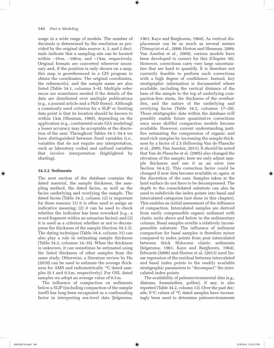
usage in a wide range of models. The number of decimals is determined by the resolution as pro-vided by the original data source: 4, 3, and 2 deci-mals indicate that a sampling site can be located within ~10 m, ~100 m, and ~1 km, respectively. Original formats are converted wherever neces-sary and, if the position is only shown on a map, this map is georeferenced in a GIS program to obtain the coordinates. The original coordinates, the reference(s), and the sample name are also listed (Table 34.1, columns 5–8). Multiple refer-ences are sometimes needed if the details of the data are distributed over multiple publications (e.g., a journal article and a PhD thesis). Although a commonly used criterion for a SLIP or limiting data point is that its location should be known to within 1 km (Shennan, 1989), depending on the application (e.g., continental-scale GIA modeling) a lesser accuracy may be acceptable at the discre-tion of the user. Throughout Tables 34.1–34.4 we have distinguished between fixed variables (i.e., variables that do not require any interpretation, such as laboratory codes) and unfixed variables that involve interpretation (highlighted by shading).
34.3.2 Sediments
The next section of the database contains the dated material, the sample thickness, the sam-pling method, the dated facies, as well as the facies underlying and overlying the sample. The dated facies (Table 34.2, column 12) is important for three reasons: (1) it is often used to assign an indicative meaning; (2) it can be used to check whether the indicator has been reworked (e.g., a wood fragment within an estuarine facies); and (3) it is used as a criterion whether or not to decom-press the thickness of the sample (Section 34.3.3). The dating technique (Table 34.4, column 31) can also play a role in estimating sample thickness (Table 34.2, columns 14–16). When the thickness is unknown, it can sometimes be estimated using the listed thickness of other samples from the same study. Otherwise, a literature review by Hu (2010) can be used to estimate the average thick-ness for AMS and radiometrically 14C dated sam-ples (0.1 and 0.5 m, respectively). For OSL dated samples we adopt an average value of 0.5 m.
The influence of compaction on sediments below a SLIP (including compaction of the sample itself) has long been recognized as a confounding factor in interpreting sea-level data (Jelgersma,
1961; Kaye and Barghoorn, 1964). As vertical dis-placement can be as much as several meters (Törnqvist et al., 2008; Horton and Shennan, 2009; Van Asselen et al., 2009), various models have been developed to correct for this (Chapter 30). However, corrections carry very large uncertain-ties that are hard to quantify. It is therefore not currently feasible to perform such corrections with a high degree of confidence. Instead, key stratigraphic information is documented where available, including the vertical distance of the base of the sample to the top of underlying com-paction-free strata, the thickness of the overbur-den, and the nature of the underlying and overlying facies (Table 34.2, columns 17–20). These stratigraphic data within the database will possibly enable future quantitative corrections once more skillful compaction models become available. However, current understanding justi-fies estimating the compression of organic and mud-rich samples by increasing the sample thick-ness by a factor of 2.5 (following Van de Plassche et al., 2005; Van Asselen, 2011). It should be noted that Van de Plassche et al. (2005) also changed the elevation of the sample; here we only adjust sam-ple thickness and use it as an error (see Section 34.4.2). This correction factor could be changed if new data become available or, again, at the discretion of the user. Samples taken at the land surface do not have to be decompressed. The depth to the consolidated substrate can also be used to subdivide the index points into basal and intercalated categories (not done in this chapter). This enables an initial assessment of the influence of compaction. Intercalated samples are derived from easily compressible organic sediment with clastic units above and below in the sedimentary column. Basal samples overlie a relatively incom-pressible substrate. The influence of sediment compaction for basal samples is therefore minor compared to index points from peat intercalated between thick Holocene clastic sediments (Jelgersma, 1961; Kaye and Barghoorn, 1964). Edwards (2006) and Horton et al. (2013) used lin-ear regression of the residual between intercalated and basal index points to the readily available stratigraphic parameters to “decompact” the inter-calated index points.
The availability of paleoenvironmental data (e.g., diatoms, foraminifera, pollen), if any, is also reported (Table 34.2, column 13). Over the past dec-ade, δ13C values of 14C dated samples have increas-ingly been used to determine paleoenvironments
0002202116.indd 540 12/8/2014 2:35:22 PM
A Protocol for a Geological Sea-Level Database 541
(Törnqvist et al., 2004; Mackie et al., 2005; Lamb et al., 2006; Engelhart et al., 2013; see also Chapter 23); δ13C values are listed in the dating section of the database (Section 34.3.4).
34.3.3 Elevation
One of the most important attributes of a SLIP or a limiting data point is the elevation from which it was sampled, as well as the elevation of the RWL. The sources of error involved in obtaining these are often underappreciated, but it is crucial to account fully for them. In the ideal scenario the elevation of the sampled indicator is measured with high-precision leveling and tied to the near-est geodetic benchmark. This will give the small-est error, although the benchmark elevation error alone can be considerable (e.g., ~0.1 m for most of the US). In some cases however, published sea-level data lack precise elevation information or the data were related to sea level, a tidal datum, or vegetation zones at the time of sampling, leading to even larger errors that can only be assessed after careful analysis of the raw data. Samples taken offshore often have large elevation errors due to corrections for waves and tides and the errors associated with the instruments measuring water depths. The surveying method (Table 34.3, col-umn 21) is therefore an essential piece of informa-tion, but frequently not described in journal articles. Depending on the surveying method used, an error is assigned (see Section 34.4.3); if the method remains unknown, a conservative error is introduced. Columns 22–25 in Table 34.3 describe the elevation of the land or subaqueous surface and the depth of the sample below this surface. The used reference level (Table 34.3, col-umn 26) for elevation measurements varies widely (e.g., from local mean sea level or MSL to a geo-detic datum). In Table 34.3, column 27 reference levels are converted – wherever necessary – to a geodetic datum (in this case, NAVD 88). One of the advantages of a geodetic/orthometric datum is that it remains constant for long periods of time and is therefore very suitable for archival pur-poses, whereas a tidal datum changes more fre-quently. To convert data that were related to tide levels we use the Vertical Datum (VDatum) Transformation tool of NOAA (2011; note that this tool is only valid for the US). With this informa-tion the elevation of the sample relative to a geo-detic datum is calculated (Table 34.3, columns 28–30). In other places where similar tools are not
available and where it is not possible to relate all data to a geodetic datum, the data should at least be related to the same tide level. The Admiralty Tide Tables produced by the United Kingdom Hydrographic Office (http://www.ukho.gov.uk/productsandservices/paperpublications/pages/nauticalpubs.aspx) provide tidal datums for all locations across the globe and are therefore very useful. It should be noted, however, that tidal ranges within estuaries and on saltmarshes are often substantially different from those on open coasts (see also Section 34.3.5).
34.3.4 Dating
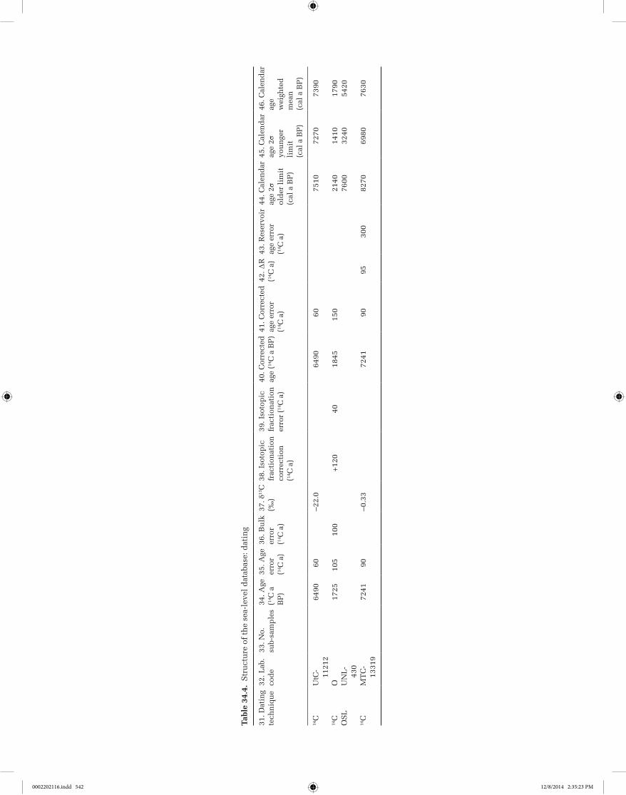
The vast majority of published, post-LGM RSL data have been dated by means of 14C (Chapter 23), 210Pb, 137Cs (Chapter 24) or U–Th (Chapter 26). In recent years, optically stimulated luminescence (OSL) dating (Chapter 27) has become more com-mon. The sea-level database reports the 2σ age errors, rounded to the nearest 10 for 14C and OSL dating (different rounding approaches may be more appropriate for other dating techniques). In the literature, OSL and U–Th ages are usually given with their 1σ analytical error so that value should be doubled. For 14C analysis, dating accu-racy is at least as important as analytical precision and depends on the nature of the dated material, reservoir effects, and uncertainties associated with isotopic fractionation correction (below and Chapter 23).
The laboratory code (Table 34.4, column 32) provides critical information about where and when the sample was dated. In some cases this is crucial as different laboratories use different pro-tocols. A good example is the correction of 14C ages for isotopic fractionation (based on δ13C measurements). This had become a standard pro-cedure at most laboratories by the late 1970s (Stuiver and Polach, 1977), but some laboratories have only applied this correction since the mid-1980s. With the laboratory code it can be verified with the laboratories, in principle, whether or not this correction has been applied. Uncorrected sea-level data have potentially large uncertainties as the fractionation effect can – if unaccounted for – lead to age offsets of hundreds of 14C years. The necessary correction depends on the dated mate-rial and is detailed in Chapter 23. The δ13C value of a sample (Table 34.4, column 37) gives impor-tant information about the amount of fractiona-tion and, if available, should be listed. However,
0002202116.indd 541 12/8/2014 2:35:23 PM
Tabl
e 34
.4.
Str
uct
ure
of
the
sea-
leve
l d
atab
ase:
dat
ing
31. D
atin
g te
chn
iqu
e32
. Lab
. co
de
33. N
o.su
b-sa
mp
les
34. A
ge(14
C a
B
P)
35. A
ge
erro
r(14
C a
)
36. B
ulk
erro
r (14
C a
)
37. δ
13C
(‰)
38. I
soto
pic
frac
tion
atio
nco
rrec
tion
(14
C a
)
39. I
soto
pic
frac
tion
atio
ner
ror
(14C
a)
40. C
orre
cted
ag
e (14
C a
BP
)41
. Cor
rect
ed
age
erro
r
(14C
a)
42. ∆
R(14
C a
)43
. Res
ervo
irag
e er
ror
(14
C a
)
44. C
alen
dar
ag
e 2σ
old
er l
imit
(cal
a B
P)
45. C
alen
dar
ag
e 2σ
you
nge
r li
mit
(cal
a B
P)
46. C
alen
dar
ag
ew
eigh
ted
m
ean
(cal
a B
P)
14C
UtC
-11
212
6490
60–2
2.0
6490
6075
1072
7073
90
14C
O17
2510
510
0+
120
4018
4515
021
4014
1017
90O
SL
UN
L-
430
7600
3240
5420
14C
MT
C-
1331
972
4190
–0.3
372
4190
9530
082
7069
8076
30
0002202116.indd 542 12/8/2014 2:35:23 PM
A Protocol for a Geological Sea-Level Database 543
whenever this value is known the correction has almost certainly been carried out. In addition, due to the fact that isotopic fractionation correction was not adopted by all dating laboratories simul-taneously, an error should be assigned to samples where it is unknown whether a correction was performed. This error (σI) is defined (see also Chapter 23):
σ σI i it= +∆ (34.2)
where Δti represents the isotopic fractionation correction for the specific dated material (Table 34.4, column 38) and σi represents the asso-ciated fractionation correction error (Table 34.4, column 39; Fig. 34.2).
Table 34.4, columns 34 and 35 list the 14C age and the associated analytical error. Sometimes multiple 14C ages are obtained from the same layer (e.g., several dated macrofossils from a thin peat bed) that can be combined to a single 14C age with a smaller error (the calculation of weighted mean 14C ages is discussed in Chapter 23). The number of subsamples is listed in Table 34.4, column 33. Since the development of accelerator mass spec-trometry (AMS), the potential for using small 14C samples has increased. Several studies have dem-onstrated that for organic material (notably peat), AMS 14C dating of plant macrofossils provides better constrained ages than bulk peat samples (Chapter 23) and it is now the preferred method. Based on a recent quantitative analysis (Hu, 2010), a “bulk error” of ±100 14C a (Table 34.4, column 36) is applied to bulk peat samples (Fig. 34.2); we adopt the same additional error for bulk shell
samples. Note that this does not mean that all con-ventional ages receive this extra bulk error; if a single wood or shell fragment was 14C dated con-ventionally such an additional error is not necessary.
Finally, 14C dated samples can be subject to a reservoir effect (marine or estuarine; see Chapter 23). Values reported by the original authors on local reservoir effects should be used wherever available (unless new data have become available since publication). It is often underap-preciated how variable reservoir effects can be on a regional scale, compared to the global average marine reservoir effect of 405 ± 22 14C a (Reimer et al., 2009). This should be verified with the online database of Reimer and Reimer (2001) where end-member values are often estuarine rather than marine (and hence particularly rele-vant to sea-level studies). In estuaries, the reser-voir effect is influenced by the level of mixing between marine waters and freshwater that may or may not be significantly depleted in 14C (depending on the nature of source rocks). Also, reservoir effects have in many cases been subject to changes through time (McGregor et al., 2008; Yu et al., 2010). Table 34.4, column 42 lists the ∆R value which is the deviation of the local reservoir effect from the global average (e.g., a reservoir effect of 500 14C a corresponds to a ∆R of 95 14C a) and is often an input variable in calibration soft-ware. The error associated with the reservoir age (Table 34.4, column 43) can vary widely, depend-ing on the available data.
For calibrating 14C ages, several programs are available (Chapter 23). We prefer OxCal (Bronk
2.2 1.41.61.82.0
–0.75
–2.00
–1.00
–1.25
–1.50
–1.75
A
B
Age (cal ka BP)
RS
L (m
)
–2.25
A: 1725 ± 105 14C a BP; 1880-1400 cal a BP, weighted mean 1640 cal a BP; RSL: -0.81 to -1.00 m Brackish peat
B: 1845 (1725+120) ± 150 (1052+1002+402)0.5 14C a BP; 2130-1410 cal a BP, weighted mean 1770 cal a BP ; RSL: -2.02 to - 0.76 m
Fig. 34.2. Comparison of error ellipses obtained without (Ellipse A) and with (Ellipse B) a comprehensive error analysis. Ellipse A shows sample 2 (Table 34.1) of Coleman and Smith (1964) based on their reported 14C age and vertical error, and the inferred RWL at MHW. Ellipse B shows the result for the same sample following the database protocol described in this chapter. Because it is a brackish peat, 120 ± 40 14C a is added to correct for isotopic fractionation (Chapter 23). Furthermore, a bulk error of ±100 14C a is added. The vertical error increases significantly, because we determine RWL as the midpoint between HAT and MTL, and the uncertainties in the sample elevation (±0.5 m) and the IR (±0.23 m) are relatively large. Error calculations in both the vertical and horizontal direction are based on Equation 34.2. The black squares indicate the points with maximum probability density.
0002202116.indd 543 12/8/2014 2:35:23 PM
544 Part 4: Modeling
Ramsey, 1995, 2009) as it provides weighted means for the calibrated age. Results from other dating techniques that do not require calibration (e.g., OSL) are listed in Table 34.4, columns 44–46. If a bulk or isotopic fractionation correction is required, a corrected 14C age is calculated prior to calibration. Estuarine and marine carbonate ages are calibrated with the Marine13 curve (Reimer et al., 2013) using the appropriate ∆R value and error, while all other samples are calibrated with the IntCal13 curve (Reimer et al., 2013). Some organisms (e.g., algal mats) can take up both ter-restrial and marine carbon and a mix of the Marine13 and IntCal13 curves can be used (e.g., Livsey and Simms, 2013). Many studies in the past did not correct marine carbonates for isotopic fractionation and reservoir effects; because they are of similar magnitude but opposite sign, they approximately cancel each other out. This results in a mean of the calibrated age range that may be accurate, but with a significantly underestimated error.
34.3.5 Tidal parameters
SLIPs are defined with respect to specified tidal datums (e.g., MTL or MSL). The traditional approach (e.g., Shennan, 1982) has been to use a nearby tide gauge record to quantify these datums before application to geological sea-level data. The limitation of this approach is twofold: (1) tide gauges are not always available near the site, meaning that distant or open coast data may have to be relied upon although the sample may have formed further inshore; and (2) tidal range may have changed significantly since the sample was formed, particularly during the middle and early Holocene (Van der Molen and De Swart, 2001; Uehara et al., 2006; Griffiths and Peltier, 2009; Hill et al., 2011). Although for many places around the globe tide gauge data remain the only option, (paleo)tidal modeling (Chapter 29) is an increas-ingly used and powerful tool. Here, we
incorporate the tidal model of Hill et al. (2011). The model resolves the issue of distant tide gauge data as it provides tidal data for any given location off the US Gulf and Atlantic coastline for the past 10 cal ka at 1 cal ka intervals. This model (see Chapter 29 for an indepth description) can accu-rately reproduce modern observations from tide gauge records.
With this model we calculated tide levels for the modern situation (Table 34.5, columns 47–53) and for the appropriate paleo-time interval for each database entry, relative to a geodetic datum. Since we use modern data to calculate the RWL (see below), we do not list all paleotidal data in the table. Since many sea-level data are collected on land, we had to extrapolate the tidal data onshore (Fig. 34.3). We assume the calculation for 1000 cal a BP to be valid for the period 501–1500 cal a BP and follow this principle through-out, with two exceptions. First, since the modeled change in tidal range between 8000 and 9000 cal a BP is linked to the opening of the Hudson Strait between 8450 and 8300 cal a BP (Hill et al., 2011; Törnqvist and Hijma, 2012), we link all samples dated to 7501–8300 cal a BP to the model output for 8000 cal a BP and samples dated to 8301–9500 cal a BP to the output for 9000 cal a BP. Any future refinement or change in the timing of the opening of the Hudson Strait may require a modi-fication to this exception. Furthermore, all sam-ples dated older than 9501 cal a BP are linked to the 10,000 cal a BP output.
Paleotidal models predict tide levels using bathy-metries based on GIA models, which should pro-duce good approximations for open marine tides. However, modeling a large region requires compro-mise, most notably in under-resolving complex nearshore bathymetry and coastal features. The inland propagation of the tidal wave is therefore not modeled accurately. Also, the models do not account for sedimentation or erosion (Shennan and Horton, 2002), which will have a significant impact on the accuracy of tidal datums in nearshore
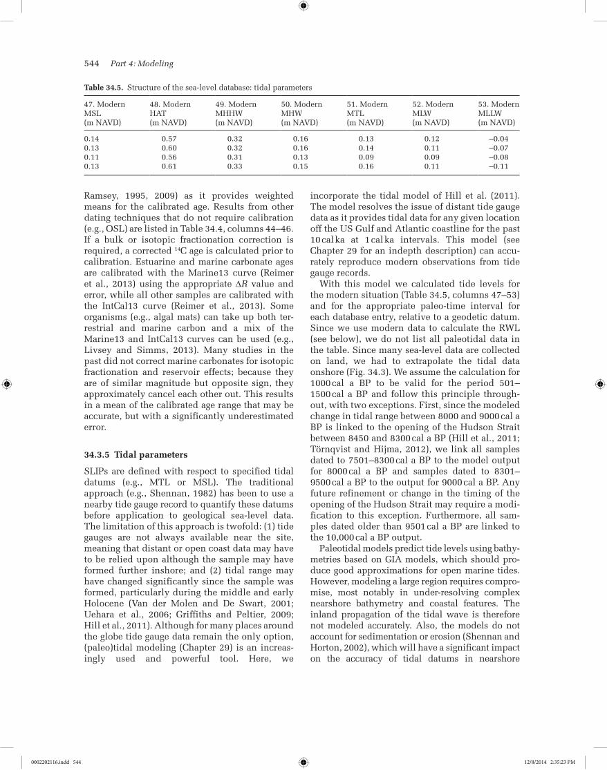
Table 34.5. Structure of the sea-level database: tidal parameters
A Protocol for a Geological Sea-Level Database 545
settings. For databases that cover large areas it is therefore best to use the tidal modeling results for the present-day situation to calculate RWL and IR when calculating paleo-RSL. We then compare the modern and the paleo-IR for each sample and incorporate the difference as an additional error (Section 34.4.1). This means that we restrict the application of paleotidal modeling to an error esti-mate rather than to adjust the elevation of paleo-RSL. This approach also avoids circularity problems: paleobathymetries used in paleotidal models are often solely based on GIA models that are calibrated and validated with RSL data.
In more local sea-level studies there are often better constraints on the paleogeography, and bathymetries can be estimated from local data rather than GIA models (e.g., Shennan et al., 2003; Hall et al., 2013). In those cases it is possible to fine-tune a tidal model to smaller areas (~100 km across) such that the results are reliable enough to use paleotidal data to correct the elevation of SLIPs and limiting data (Horton et al., 2013). In regions where similar models as that of Hill et al. (2011) exist or are being developed, the same methodology as used here can be applied. Where tidal models do not currently exist, tide gauge data must still be employed. The Admiralty Tide Tables provide this type of information. The tide gauge nearest to the sampling site is useful
when it is located, for instance, within the same bay. In other cases the average of the nearest two (one on each side of the sampling site) should be used (e.g., Shennan, 1982), with half the differ-ence as an error.
A substantial number of SLIPs formed inshore (e.g., small bays, marshes) and hence in environ-ments where the tidal datums could have been substantially different (in most cases lower) than at nearshore sites, where large-scale tidal models give the best results and where most tide gauges are situated. This means that in most cases the tidal range error is overestimated (Hijma and Cohen, 2010). In deltas, the inland propagation of the tidal wave is also influenced by the river- gradient effect (Van de Plassche, 1982) that raises the elevation of the tidal datums (see also Chapter 33).
34.3.6 Indicative range, reference water level, and relative sea level
Based on all the paleoenvironmental and strati-graphic information (Table 34.2, columns 13–20) we label each data entry as either a SLIP or an upper or lower limiting data point (Table 34.6, column 54). For each SLIP the IR is calculated (Table 34.6, columns 55–57), based on the paleoen-vironment in which the sea-level indicator formed (see also Fig. 34.1). Along the US Atlantic and
Fig. 34.3. (a) Modeled present-day tidal range (MHHW – MLLW) in the NW Gulf of Mexico. Black dots show the location of SLIPs and limiting data. (b) Tidal range for the entire block with extrapolated values for the onshore portions, enabling the calculation of tidal parameters for sampling sites on land. The offshore part of (b) does not match (a) exactly due to slightly different smoothing parameters. This was necessary because in the data for (a) there were some non-realistic values in regions where nodes are occasionally dry. For those nodes, traditional harmonic analysis is not feasible (see also Chapter 29). To prevent those nodes from influencing the extrapolation, some smoothing was performed on (a) before extrapolation; the panels are therefore not identical for the offshore area. For color details, please see Plate 46.
(a)
–98 –92–94–96
Longitude
0.7
0
0.1
0.2
0.3
0.4
0.5
0.6
Tidal range (m)
24
26
28
30La
titud
e(b)
–98 –92–94–96
Longitude
0.7
0
0.1
0.2
0.3
0.4
0.5
0.6
Tidal range (m)30
24
26
28
Latit
ude
0002202116.indd 545 12/8/2014 2:35:24 PM
546 Part 4: Modeling
Gulf coasts, the majority of sea-level indicators formed within saltmarshes or brackish marshes. Within a saltmarsh it is usually possible to observe a clear vertical zonation of plants into high-marsh and low-marsh zones (and in some instances more) that reflect the preferences and tolerances of halophytic species to the frequency and dura-tion of tidal inundation between MTL and HAT. If preserved plant macrofossils or microfossils sug-gest a high-saltmarsh environment, an IR of MHW to HAT is assigned. For low-saltmarsh environ-ments, the IR applied is MTL to MHW.
As outlined above we use modeled present-day tidal data to calculate RWL (Table 34.6, columns 55–56) and incorporate the paleotidal model results into the error (Section 34.4.1). We do this based on a comparison of the modern and paleo-IR (Table 34.6, columns 57–58). The latter is cal-culated using the modeled paleotidal data. In studies that apply the highest possible standards to minimize other elevation errors associated with sampling and surveying, the IR typically ends up being the main contributor to the vertical uncer-tainty. With RWL and Equation 34.1 we calculate paleo-RSL for the SLIPs (Table 34.8, column 74). For limiting data we also use Equation 34.1, but in these cases we label the outcome as limiting-data elevation (Table 34.8, column 75).
34.4 VERTICAL ERRORS
So far, we have described the database structure in general terms, including the steps involved in cal-culating paleo-RSL or the elevation of limiting data. This section focuses specifically on vertical error calculations. Wherever a publication provides suf-ficiently specific information on such errors, that information trumps any standardized error esti-mates as outlined below. Note that not all listed errors apply in every case. For the summation of errors we use the commonly applied expression:
E e e ent = + + +( )12
22 2 (34.3)
where e1…en are component errors and Et is the total error. This is the same equation as that used for the 14C age error calculation (Chapter 23).
While the 2σ age error is statistically rigorous, the confidence interval associated with the verti-cal error is less well defined. Nevertheless, we aim for a reasonable approximation of a 2σ error by assessing all vertical errors very conservatively. Total upward and downward errors are computed separately (Table 34.8, columns 76, 77), because the non-vertical drilling error (Table 34.8, column 67) is unidirectional.
To plot SLIPs we prefer to use shapes that approximate ellipses (also referred to as “blobs”; Chapter 32) defined by the 2σ horizontal (age) error range and the 2σ vertical (elevation) error range (Fig. 34.2). Ellipses represent the 2σ error of SLIPs better than the frequently used error boxes. While the SLIPs illustrated here (Figs 34.2 and 34.4b) are represented by ellipses, it should be noted that the point of maximum probability den-sity is commonly not located exactly in their cent-ers (both the horizontal and vertical errors are often asymmetric). In other words, a more accu-rate geometric representation that accounts for these (often slight) asymmetries would constitute a further improvement.
For limiting data points, several symbols have been used in the literature (e.g., boxes, crosses, T-shaped symbols). Here we use T-shaped sym-bols with the horizontal bar placed at the extreme end of the vertical 2σ error range. For upper limit-ing data points the horizontal bar lies at the top, while for lower limiting data points the horizontal bar lies at the base of this range. The width of the horizontal bar is defined by the horizontal 2σ error range. It is important to bear in mind that, in the case of an upper limiting data point, MSL is inter-preted to have been below the horizontal line merely at some point along its full width. If infor-mation about the length of the vertical error range is to be included, a T-shape should be used for upper limiting data (Fig. 34.4b), while a ⊥-shape should be used for lower limiting data. The length
Table 34.6. Structure of the sea-level database: reference water level and indicative range
54. Classification 55. RWL 56. Modern RWL (m NAVD) 57. Modern IR (m) 58. Paleo-IR (m)
of the vertical bar is then defined by the vertical error range and points (by means of an arrow) in the direction of paleo-RSL; its position is defined by the weighted mean calendar age. Other studies (e.g., Engelhart and Horton, 2012) have used a T-shape for lower limiting data and a ⊥-shape for upper limiting data to avoid confusion with coral-based RSL reconstruction usage (e.g., Peltier and Fairbanks, 2006) where the vertical bar is used to define the living range of coral species and with the RSL curve expected to pass through the bar. The position of the horizontal bar in their analysis is similar as in the present protocol, but the length of the vertical bar is not defined by the magnitude of the vertical error.
34.4.1 Indicative meaning related errors
In the following sections, all errors related to spe-cific parts of the database are discussed using numbered lists.
(1) The IR error is defined as half the IR (Table 34.7, column 59).
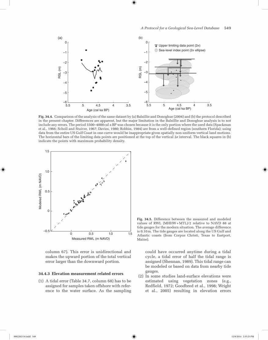
(2) The error associated with the modeled RWL is based on a comparison of predictions with the model of Hill et al. (2011) for 40 tide gauges from Texas to Maine using MTL to mean higher high water (MHHW) as the IR (HAT was not always available) and the measured values at those stations. The average differ-ence between the modeled and measured RWL is 0.10 m; we therefore adopt an error of ±0.10 m for the RWL (Fig. 34.5; Table 34.7, col-umn 60). Since the average difference between the modeled and measured IR is 20% of the modern IR, we use this to calculate the IR error (Table 34.7, column 61). In other regions where other models may be used, these errors can be substantially different.
(3) The IR change error accounts for the differ-ence between the modern IR and the paleo-IR.
It is defined as half the difference between the modern IR and the paleo-IR (Table 34.7, col-umn 62) and also applies to cases where the paleo-IR is smaller than the modern IR.
(4) For sites that were not linked to a geodetic datum by the original authors, we converted the elevation using VDatum (NOAA, 2011). The average difference between VDatum com-putations for MSL relative to NAVD 88 at tide gauges and the actual data from those stations is ±0.05 m (Fig. 34.6; Table 34.7, column 63; see also http://vdatum.noaa.gov/docs/est_uncertainties.html). VDatum can also be used to convert elevations that were related to the older National Geodetic Vertical Datum of 1929. In other regions a different approach using Admiralty Tide Tables or local data will change this error.
34.4.2 Sampling related errors
(1) The thickness error (Table 34.7, column 64) is defined as half the thickness of the sample (Shennan, 1986). If the sample was decom-pressed (Section 34.3.3) we calculate this error using the corrected sample thickness (Table 34.2, column 17).
(2) Sampling errors (Table 34.7, column 65) arise from measuring the sample depth within a core or section. They are often not reported, but can be considered small. We use ±0.01 m, following Shennan (1986).
(3) Core stretching/shortening errors (Table 34.7, column 66) can be quite substantial, espe-cially for rotary coring and vibracoring. According to Morton and White (1997), up to 30% of core shortening can occur within a sampling interval of less than 1 m; on the other hand, alternating unshortened and shortened sampling intervals are commonly observed. We set the error at ±0.15 m for rotary coring and vibracoring (Morton and White, 1997), ±0.05 m for hand coring (Woodroffe, 2006) and ±0.01 m for a Russian sampler (Woodroffe, 2006).
(4) Non-vertical drilling makes the apparent depth of a sample larger than the true depth, with discrepancies increasing with drilling depth. According to Törnqvist et al. (2004), the resulting error may be as large as –0.02 m per meter depth of hand coring. Assuming this error is similar for other coring methods, we assign an error of 0.02 m m–1 depth (Table 34.7,
Table 34.8. Structure of the sea-level database: paleo-RSL calculation
74. Paleo-RSL (m)
75. Limiting-data elevation (m)
76. Total upward error (m)
77. Total downward error (m)
–8.61 0.36 0.29–1.39 0.63 0.63
–1.89 0.54 0.54–12.96 0.62 0.58
0002202116.indd 548 12/8/2014 2:35:24 PM
A Protocol for a Geological Sea-Level Database 549
column 67). This error is unidirectional and makes the upward portion of the total vertical error larger than the downward portion.
34.4.3 Elevation measurement related errors
(1) A tidal error (Table 34.7, column 68) has to be assigned for samples taken offshore with refer-ence to the water surface. As the sampling
could have occurred anytime during a tidal cycle, a tidal error of half the tidal range is assigned (Shennan, 1989). This tidal range can be modeled or based on data from nearby tide gauges.
(2) In some studies land-surface elevations were estimated using vegetation zones (e.g., Redfield, 1972; Goodbred et al., 1998; Wright et al., 2005) resulting in elevation errors
Fig. 34.4. Comparison of the analysis of the same dataset by (a) Balsillie and Donoghue (2004) and (b) the protocol described in the present chapter. Differences are apparent, but the major limitation in the Balsillie and Donoghue analysis is to not include any errors. The period 5500–4000 cal a BP was chosen because it is the only portion where the used data (Spackman et al., 1966; Scholl and Stuiver, 1967; Davies, 1980; Robbin, 1984) are from a well-defined region (southern Florida); using data from the entire US Gulf Coast in one curve would be inappropriate given spatially non-uniform vertical land motions. The horizontal bars of the limiting data points are positioned at the top of the vertical 2σ interval. The black squares in (b) indicate the points with maximum probability density.
3.544.555.5−6
−5
−4
−3
−2
−1
0
Age (cal ka BP)
RS
L (m
)
(a)
3.544.555.5−6
−5
−4
−3
−2
−1
0
Age (cal ka BP)
RS
L (m
)
Upper limiting data point (2σ)
Sea-level index point (2σ ellipse)
(b)
Measured RWL (m NAVD)
Mod
eled
RW
L (m
NA
VD
)
0 0.5 1.0 1.5–0.5
1.0
0.5
0
1.5
y=x
Fig. 34.5. Difference between the measured and modeled values of RWL (MHHW + MTL)/2 relative to NAVD 88 at tide gauges for the modern situation. The average difference is 0.10 m. The tide gauges are located along the US Gulf and Atlantic coasts (from Corpus Christi, Texas to Eastport, Maine).
0002202116.indd 549 12/8/2014 2:35:25 PM
550 Part 4: Modeling
(Table 34.7, column 69) of ±0.5 m. In areas with a high tidal range this error could be larger (Engelhart, 2010).
(3) The elevation of the land surface is frequently not reported but, if the coordinates of the sam-pling site are known, the elevation can be approximated using high-resolution digital elevation models (DEMs) wherever available. The associated error does not only depend on the vertical accuracy of the DEM (often of the order 0.1–0.2 m), but also on the accuracy of the coordinates. In areas with significant relief, such as strand plains with beach ridges, this matters when the sample was taken from a ridge, but the coordinate points towards a swale. An error of ±0.5 m is assigned (Table 34.7, column 70). If conventional topo-graphic maps are used instead of DEMs, the error is half the contour-line interval (±0.75 m for US topographic maps).
(4) Water depths are typically measured using fathometers, echo sounders, and poles, along with several other techniques. If not specified by the authors, we use an error of ±0.5 m (Table 34.7, column 70).
(5) The error arising during leveling (Table 34.7, column 71) with high-precision (e.g., total sta-tion) equipment is, if unknown, set at ±0.03 m (Törnqvist et al., 2004).
(6) The standard error (Table 34.7, column 72) of a (D)GPS base station that is often used during surveying is ±0.1 m, but if carefully used the error can be as low as 0.04 m (Törnqvist et al., 2004). Care must be taken to ensure the accuracy of the D(GPS), especially in regions with varia-ble satellite coverage or restricted reception.
(7) The US National Geodetic Survey (NGS) benchmark elevations are subject to an error (Table 34.7, column 73) of ±0.1 m (Engelhart, 2010) for the most reliable and stable bench-marks. For less reliable benchmarks this error is larger. Note that the error for benchmark elevations can be different in other regions.
Again, we stress here that the standardized errors should only be used if no sufficient infor-mation was provided in the original source. If spe-cific information is published or can be obtained by other means (e.g., directly from the author(s)), that information overrules the standardized errors discussed above. This means that all errors should be assessed on a case-by-case basis.
34.5 DISCUSSION
While a long history exists of compiling geological sea-level databases for a variety of applications, relatively few have involved a com-prehensive and rigorous assessment of elevation and age errors associated with the underlying data. Here we present the most comprehensive approach to sea-level database construction to date, with a number of error sources (notably asso-ciated with dating errors and tidal range uncer-tainties) that have previously not been considered. Our approach aims to be as inclusive as possible, and we only exclude data that, according to our analysis, have no significance whatsoever with respect to past sea levels. The spirit of our approach is that any data with limited usefulness will be reflected by large vertical and/or
Longitude
0.25
0.20
0.15
0.10
0.05
092949698W 868890 84 82 80 78W
Diff
eren
ce (
m)
Fig. 34.6. Difference between the measured value of MSL at tide gauges (relative to NAVD 88) and the modeled value by Vdatum. The tide gauges are located along the US Gulf Coast, between Corpus Christi (Texas) and Lake Worth Pier (Florida). The outlier (0.22 m) is the tide gauge at Lake Charles, Louisiana, located 50 km inland of the open coast.
0002202116.indd 550 12/8/2014 2:35:25 PM
A Protocol for a Geological Sea-Level Database 551
horizontal errors. Rather than passing judgment on these data ourselves, such an assessment is then made at the discretion of the user.
By means of illustration, we compare the proto-col described above with a sea-level data analysis by Balsillie and Donoghue (2004). The latter authors compiled data (see also Donoghue, 2011) from the US Gulf Coast (separated into offshore and onshore data) and used a seven-point moving average trend line to obtain a RSL curve (Fig. 34.4a) without taking into account any errors or separat-ing between SLIPs and limiting data points. We compared our approach with theirs for the period 5500–4000 cal a BP. Using the protocol described above, it becomes apparent that several of the used indicators are freshwater peats (based on the original descriptions and/or vegetation type) and can therefore only be used as upper limiting data. The vertical 2σ errors of all data are of the order 1 m, precluding the detection of decimeter-scale sea-level fluctuations as suggested by the trend line of Balsillie and Donoghue. Where Balsillie and Donoghue interpret a RSL drop of ~1.75 m between 5000 and 4200 cal a BP, followed by a very rapid RSL rise, our analysis shows that many more interpretations are possible: sea level was somewhere between –6 m and –2 m from 5500 to 3700 cal a BP, most likely with a net RSL rise (Fig. 34.4b). The hallmark of our approach is that assigning conservative errors minimizes the risk of over-interpreting RSL records.
As outlined above, insight into the role of changes in the paleotidal regime is crucial when interpreting sea-level data. Although we use a high-resolution tidal model, we still choose to incorporate any differences between the modern and paleotidal regime as an error instead of adjust-ing RWL. The main reason for this is that the model covers a very wide region and does not incorporate paleogeographic changes on a local scale which are critical for understanding a local tidal regime. Paleotidal models that are fine-tuned to take into account paleogeographic changes can be used to adjust RWL to get more insight into local RSL changes (e.g., Shennan et al., 2003; Hall et al., 2013).
Finally, when our database protocol is used to analyze published data, newly calculated errors will differ from those in the original publications; in most cases, they will be larger (Fig. 34.2). This could lead to new insights such as revised rates of RSL change, and hence different conclusions. This obviously does not mean that previous
studies were executed poorly; it is merely a step forward in the error analysis of sea-level data. Our goal is that the protocol presented here be adopted more widely, and a start is made with the analysis of the wealth of existing geological sea-level data in a uniform way. In order to be widely used, it will become necessary for the database to be stored online. The longer-term goal is for research-ers to have the opportunity to directly upload their sea-level data, analyzed using the protocol described here, to this database.
REFERENCES
Balsillie, J.H., and Donoghue, J.F. (2004) High resolution sea-level history for the Gulf of Mexico since the last glacial maximum. Report of investigation. Florida Geological Survey, Tallahassee.
Blum, M.D., Sivers, A.E., Zayac, T., and Goble, R.J. (2003) Middle Holocene sea-level and evolution of the Gulf of Mexico Coast. Gulf Coast Association of Geological Societies, Transactions, 53, 64–77.
Bronk Ramsey, C. (1995) Radiocarbon calibration and anal-ysis of stratigraphy: The OxCal program. Radiocarbon, 37(2), 425–430.
Bronk Ramsey, C. (2009) Bayesian analysis of radiocarbon dates. Radiocarbon, 51(1), 337–360.
Coleman, J.M., and Smith, W.G. (1964) Late recent rise of sea level. Geological Society of America Bulletin, 75(9), 833–840.
Davies, T.D. (1980) Peat formation in Florida Bay and its significance in interpreting the recent vegetational and geological history of the bay area. PhD thesis, Pennsylvania State University.
Donoghue, J.F. (2011) Sea level history of the northern Gulf of Mexico coast and sea level rise scenarios for the near future. Climatic Change, 107(1–2), 17–33.
Dutton, A., and Lambeck, K. (2012) Ice volume and sea level during the last interglacial. Science, 337(6091), 216–219.
Edwards, R.J. (2006) Mid-to late-Holocene relative sea-level change in southwest Britain and the influence of sediment compaction. The Holocene, 16(4), 575–587.
Engelhart, S.E. (2010) Sea-level changes along the U.S. Atlantic coast: implications for glacial isostatic adjust-ment models and current rates of sea-level change. PhD thesis, University of Pennsylvania.
Engelhart, S.E., and Horton, B.P. (2012) Holocene sea level database for the Atlantic coast of the United States. Quaternary Science Reviews, 54, 12–25.
Engelhart, S.E., Horton, B.P., Douglas, B.C., Peltier, W.R., and Törnqvist, T.E. (2009) Spatial variability of late Holocene and 20th century sea-level rise along the Atlantic coast of the United States. Geology, 37(12), 1115–1118.
Engelhart, S.E., Horton, B.P., Vane, C.H., Nelson, A.R., Witter, R.C., Brody, S.R., and Hawkes, A.D. (2013) Modern foraminifera, δ13C, and bulk geochemistry of central Oregon tidal marshes and their application in
Flemming, N.C. (1982) Multiple regression analysis of earth movements and eustatic sea-level change in the United Kingdom in the past 9000 years. Proceedings of the Geologists’ Association, 93(1), 113–125.
Gesch, D. (2007) The National Elevation Dataset. In: Digital Elevation Model Technologies and Applications: The DEM User Manual, 2nd edition (ed. Maune, D.), American Society for Photogrammetry and Remote Sensing, Bethesda, Maryland, USA, 99–118.
Goodbred, S.L., Wright, E.E., and Hine, A.C. (1998) Sea-level change and storm-surge deposition in a late Holocene Florida salt marsh. Journal of Sedimentary Research, 68(2), 240–252.
Griffiths, S.D., and Peltier, W.R. (2009) Modeling of polar ocean tides at the last glacial maximum: amplification, sensitivity, and climatological implications. Journal of Climate, 22(11), 2905–2924.
Hall, G.F., Hill, D.F., Horton, B.P., Engelhart, S.E., and Peltier, W.R. (2013) A high-resolution study of tides in the Delaware Bay: Past conditions and future scenarios. Geophysical Research Letters, 40(2), 338–342.
Hijma, M.P., and Cohen, K.M. (2010) Timing and magni-tude of the sea-level jump preluding the 8200 yr event. Geology, 38(3), 275–278.
Hill, D.F., Griffiths, S.D., Peltier, W.R., Horton, B.P., and Törnqvist, T.E. (2011) High-resolution numerical mod-eling of tides in the western Atlantic, Gulf of Mexico, and Caribbean Sea during the Holocene. Journal of Geophysical Research, 116, C10014.
Horton, B.P., and Shennan, I. (2009) Compaction of Holocene strata and the implications for relative sea-level change on the east coast of England. Geology, 37(12), 1083–1086.
Horton, B.P., Engelhart, S.E., Hill, D.F., Kemp, A.C., Nikitina, D., Miller, K.G., and Peltier, W.R. (2013) Influence of tidal-range change and sediment compac-tion on Holocene relative sea-level change in New Jersey, USA. Journal of Quaternary Science, 28(4), 403–411.
Hu, P. (2010) Developing a quality-controlled postglacial sea-level database for coastal Louisiana to assess con-flicting hypotheses of Gulf Coast sea-level change. MSc thesis, Tulane University, New Orleans.
Jelgersma, S. (1961) Holocene sea-level changes in The Netherlands. Mededelingen Geologische Stichting, 7, 1–101.
Kaye, C.A., and Barghoorn, E.S. (1964) Late Quaternary sea-level change and crustal rise at Boston, Massachusetts, with notes on the autocompaction of peat. Geological Society of America Bulletin, 75(2), 63–80.
Lamb, A.L., Wilson, G.P., and Leng, M.J. (2006) A review of coastal palaeoclimate and relative sea-level reconstruc-tions using δ13C and C/N ratios in organic material. Earth-Science Reviews, 75(1–4), 29–57.
Lambeck, K., Smither, S., and Johnston, P. (1998) Sea-level change, glacial rebound and mantle viscosity for Northern Europe. Geophysical Journal International, 134, 102–144.
Lambeck, K., Anzidei, M., Antonioli, F., Benini, A., and Esposito, A. (2004) Sea level in Roman time in the
Central Mediterranean and implications for recent change. Earth and Planetary Science Letters, 224(3–4), 563–575.
LaSalle, M.W., and Parsons, J. (1985) Species profiles: life histories and environmental requirements of coastal fishes and invertebrates (Gulf of Mexico). Common Rangia, 82, 1–18.
Lighty, R.G., Macintyre, I.G., and Stuckenrath, R. (1982) Acropora palmata reef framework: A reliable indicator of sea level in the western atlantic for the past 10,000 years. Coral Reefs, 1(2), 125–130.
Livsey, D., and Simms, A.R. (2013) Holocene sea-level change derived from microbial mats. Geology, doi: 10.1130/G34387.1.
Mackie, E.A.V., Leng, M.J., Lloyd, J.M., and Arrowsmith, C. (2005) Bulk organic δ13C and C/N ratios as palaeosalin-ity indicators within a Scottish isolation basin. Journal of Quaternary Science, 20(4), 303–312.
McGregor, H.V., Gagan, M.K., McCulloch, M.T., Hodge, E., and Mortimer, G. (2008) Mid-Holocene variability in the marine 14C reservoir age for northern coastal Papua New Guinea. Quaternary Geochronology, 3(3), 213–225.
Milliken, K.T., Anderson, J.B., and Rodriguez, A.B. (2008) A new composite Holocene sea-level curve for the northern Gulf of Mexico. In: Response of Upper Gulf Coast Estuaries to Holocene Climate Change and Sea-Level Rise (eds Anderson, J.B., and Rodriguez, A.B.), Geological Society of America, Special Paper 443, 1–11.
Milne, G., Long, A., and Bassett, S. (2005) Modelling Holocene relative sea-level observations from the Caribbean and South America. Quaternary Science Reviews, 24, 1183–1202.
Morton, R.A., and White, W.A. (1997) Characteristics of and corrections for core shortening in unconsolidated sediments. Journal of Coastal Research, 13(3), 761–769.
NOAA (2011) Vertical Datum Transformation. Available at http://vdatum.noaa.gov/welcome.html (accessed 4 August 2014).
Peltier, W.R., and Fairbanks, R.G. (2006) Global glacial ice volume and Last Glacial Maximum duration from an extended Barbados sea level record. Quaternary Science Reviews, 25(23–24), 3322–3337.
Peltier, W.R., Shennan, I., Drummond, R., and Horton, B. (2002) On the postglacial isostatic adjustment of the British Isles and the shallow viscoelastic structure of the Earth. Geophysical Journal International, 148, 443–475.
Redfield, A.C. (1972) Development of a New England salt marsh. Ecological Monographs, 42, 201–201.
Reimer, P.J., and Reimer, R.W. (2001) A marine reservoir correction database and on-line interface. Radiocarbon, 43, 461–463.
Reimer, P.J., Baillie, M.G.L., Bard, E. et al. (2009) IntCal09 and Marine09 radiocarbon age calibration curves, 0-50,000 years cal BP. Radiocarbon, 51(4), 1111–1150.
Reimer, P.J., Bard, E., Bayliss, A. et al. (2013) IntCal13 and Marine13 radiocarbon age calibration curves 0-50,000 yr cal BP. Radiocarbon, 55(4), 1869–1887.
Robbin, D.M. (1984) A new Holocene sea level curve for the Upper Florida Keys and Florida reef tract. In: Environments of South Florida: Present and Past II. (ed.
0002202116.indd 552 12/8/2014 2:35:25 PM
A Protocol for a Geological Sea-Level Database 553
Scholl, D.W., and Stuiver, M. (1967) Recent submergence of Southern Florida: A comparison with adjacent coasts and other eustatic data. Geological Society of America Bulletin, 78(4), 437–454.
Shennan, I. (1982) Interpretation of Flandrian sea-level data from the Fenland, England. Proceedings of the Geologists’ Association, 93(1), 53–63.
Shennan, I. (1986) Flandrian sea-level changes in the Fenland. II: Tendencies of sea-level movement, altitudi-nal changes, and local and regional factors. Journal of Quaternary Science, 1, 155–179.
Shennan, I. (1989) Holocene crustal movements and sea-level changes in Great Britain. Journal of Quaternary Science, 4(1), 77–89.
Shennan, I., and Horton, B. (2002) Holocene land- and sea-level changes in Great Britain. Journal of Quaternary Science, 17(5–6), 511–526.
Shennan, I., Lambeck, K., Horton, B., Innes, J., Lloyd, J., McArthur, J., and Rutherford, M. (2000) Holocene isos-tasy and relative sea-level changes on the east coast of England. In: Holocene Land-Ocean Interaction and Environmental Change around the North Sea (eds Shennan, I. and Andrews, J.), Geological Society, London, Special Publications 166(1), 275–298.
Shennan, I., Coulthard, T., Flather, R., Horton, B., Macklin, M., Rees, J., and Wright, M. (2003) Integration of shelf evolution and river basin models to simulate Holocene sediment dynamics of the Humber Estuary during peri-ods of sea-level change and variations in catchment sediment supply. Science of the Total Environment, 314–316, 737–754.
Spackman, W., Dolsen, C.P., and Riegel, W. (1966) Phytogenic organic sediments and sedimentary environ-ments in the Everglades-Mangrove Complex. Part I: Evidence of a transgressing sea and its effects on envi-ronments of the shark river area of southwestern Florida. Palaeontographica Abteilung B, 117(4–6), 135–152.
Stuiver, M., and Polach, H. (1977) Discussion; reporting of C-14 data. Radiocarbon, 19(3), 355–363.
Törnqvist, T.E., and Hijma, M.P. (2012) Links between early Holocene ice-sheet decay, sea-level rise and abrupt cli-mate change. Nature Geoscience, 5, 601–606.
Törnqvist, T.E., González, J.L., Newsom, L.A., Van der Borg, K., De Jong, A.F.M., and Kurnik, C.W. (2004) Deciphering Holocene sea-level history on the US Gulf Coast: A high-resolution record from the Mississippi Delta. Geological Society of America Bulletin, 116(7), 1026–1039.
Törnqvist, T.E., Wallace, D.J., Storms, J.E.A., Wallinga, J., van Dam, R.L., Blaauw, M., Derksen, M.S., Klerks, C.J.W., Meijneken, C., and Snijders, E.M.A. (2008) Mississippi Delta subsidence primarily caused by com-paction of Holocene strata. Nature Geoscience, 1(3), 173–176.
Toscano, M.A., and Macintyre, I.G. (2003) Corrected west-ern Atlantic sea-level curve for the last 11,000 years based on calibrated Acropora Palmata framework and intertidal mangrove peat. Coral Reefs, 22, 257–270.
Troiani, B.T., Simms, A.R., Dellapenna, T., Piper, E., and Yokoyama, Y. (2011) The importance of sea-level and
climate change, including changing wind energy, on the evolution of a coastal estuary: Copano Bay, Texas. Marine Geology, 280(1–4), 1–19.
Uehara, K., Scourse, J.D., Horsburgh, K.J., Lambeck, K., and Purcell, A.P. (2006) Tidal evolution of the northwest European shelf areas from the Last Glacial Maximum to the present. Journal of Geophysical Research, 111, C09025–C09025.
Van Asselen, S. (2011) The contribution of peat compac-tion to total basin subsidence: implications for the pro-vision of accommodation space in organic-rich deltas. Basin Research, 23, 239–255.
Van Asselen, S., Stouthamer, E., and Van Asch, T.W.J. (2009) Effects of peat compaction on delta evolution: A review on processes, responses, measuring and mode-ling. Earth-Science Reviews, 92(1–2), 35–51.
Van de Plassche, O. (1982) Sea-level change and water-level movements in the Netherlands during the Holocene. Mededelingen Rijks Geologische Dienst, 36, 1–93.
Van de Plassche, O. (1986) Introduction. In: Sea-Level Research: A Manual for the Collection and Evaluation of Data. (ed. Van de Plassche, O.) Geobooks, Norwich, 1–26.
Van de Plassche, O. (1991) Late Holocene sea-level fluctua-tions on the shore of Connecticut Inferred from trans-gressive and regressive overlap boundaries in salt-marsh deposits. Journal of Coastal Research, 11, 159–179.
Van de Plassche, O., Bohncke, S.J.P., Makaske, B., and Van der Plicht, J. (2005) Water-level changes in the Flevo area, central Netherlands (5300-1500 BC): implications for relative mean sea-level rise in the Western Netherlands. Quaternary International, 133–134, 77–93.
Van der Molen, J., and De Swart, H.E. (2001) Holocene tidal conditions and tide-induced sand transport in the southern North Sea. Journal of Geophysical Research, C, 106, C5, 9339–9362.
Vink, A., Steffen, H., Reinhardt, L., and Kaufmann, G. (2007) Holocene relative sea-level change, isostatic sub-sidence and the radial viscosity structure of the mantle of northwest Europe (Belgium, the Netherlands, Germany, southern North Sea) Quaternary Science Reviews, 26(25–28), 3249–3275.
Woodroffe, S.A. (2006) Holocene relative sea-level changes in Cleveland Bay, North Queensland, Australia. PhD thesis, Durham University, Durham, UK.
Wright, E.E., Hine, A.C., Goodbred, S.L., and Locker, S.D. (2005) The effect of sea-level and climate change on the development of a mixed siliciclastic-carbonate, deltaic coastline: Suwannee River, Florida, USA. Journal of Sedimentary Research, 75(4), 621–635.
Yu, K., Hua, Q., Zhao, J.-X., Hodge, E., Fink, D., and Barbetti, M. (2010) Holocene marine 14C reservoir age variability: Evidence from 230Th-dated corals in the South China Sea. Paleoceanography, 25(3), PA3205.
Yu, S.-Y., Törnqvist, T.E., and Hu, P. (2012) Quantifying Holocene lithospheric subsidence rates underneath the Mississippi Delta. Earth and Planetary Science Letters, 331–332, 21–30.