Chapter 39: Multi-Agency Radiation Survey and Site Investigation Manual (Scenario A) The Multi-Agency Radiation Survey and Site Investigation Manual (MARSSIM) is the product of interagency cooperation among five key US federal agencies responsible for managing radioactive materials: the Department of Energy, the Department of Defense, the Environmental Protection Agency, the Nuclear Regulatory Commission, and the Department of Homeland Security. This document provides fairly detailed guidance for determining whether a site is in compliance with a radiation dose or risk-based regulation. You can obtain a copy of MARSSIM at this website http://www.epa.gov/rpdweb00/marssim/. The chapter and discussion most relevant to this user guide is found in Chapter 5 section 5 (Final Status Surveys). Also you may find the document NUREG 1505 particularly helpeful as well (http://www.orau.org/PTP/PTP%20Library/library/NRC/NUREG/NUREGS.htm). NUREG 1505 was a building block in the formation of MARSSIM and was authored by the USNuclear Regulatory Commission and the US Department of Energy. It focuses more closely on the methods we present here. This chapter is neither a substitute for any guidance document or for any official MARSSIM training. It assumes a reasonable level of knowledge about MARSSIM and shows you how to implement those features in SADA. This chapter covers those features in SADA associated with Scenario A. (The other scenario “Scenario B” is essentially the reverse hypothesis regarding contamination on site). We begin by reviewing two important principles: survey unit and release criterion. Survey Unit A survey unit is a geographical area with a specific size and shape. A survey unit may be the entire site or a smaller portion of the site. The important thing to emphasize here is that the survey unit will be the geographic target for decision making. You may have more than one survey unit on your site. Each one then becomes a separate decision. Specifically, each one must pass a release criterion in order to be released for public use. If a survey unit fails the release criterion additional steps must be taken prior to release. Release Criterion The criteria for release is that the exposure levels must be less than the total effective dose equivalent (TEDE). You can’t directly measure the exposure someone receives while interacting with the survey unit over a set time without actually exposing them to radiation. This obviously defeats the purpose of such an environmental assessment. Rather an exposure pathway model is used to model exposure over time. More importantly, an exposure model can determine the maximum allowable concentration associated with the TEDE. This concentration limit is referred to as the Derived Concentration Guideline (DCGL) and is expressed in units that can be measured now (e.g. Bq/g or Bq/m2). There are two concerns in assessing radiological contamination in MARSSIM. First, the site wide average concentration should not exceed the DCGL. For this reason, it is usually written as the DCGLw (the w indicates survey wide limit). In addition to this site-wide constraint, localized hotspots of activity may also pose a health threat. A separate DCGL known as the
DCGLemc is used to screen against local hot spot values. The two values are related to each other through the area factor. More specifically we have,
DCGLemc= FA x DCGLw The derivation of the area factor (FA) is beyond the scope of this user guide. The important point here is that we will be dealing with two decision criteria (DCGLw, DCGLemc) at two different scales (site-wide, local). For the site-wide comparison a non-parameteric test will be used. Either the Sign test or Wilcoxon Rank Sum (WRS) test will be used to test the hypothesis that the site-wide average is less than the DCGLw. Comparisons for the local activity levels will be conducted by comparing scanning results and/or sample measurements directly against the DCGLemc. Any result that exceeds the DCGLemc, raises concerns about the safety of the site. The number of samples you will need to take represents a balance between these two separate objectives. We will now discuss laying out samples in order to apply these two decision approaches simultaneously. Classifying the Survey Unit Survey units are classified according the liklihood that they are contaminated. More sampling resources will be spent on the most contaminated units. Class I Areas These are areas containing locations where, prior to remediation, the concentrations of residual radioactivity may have exceeded the DCGLW. Class I areas have the highest potential for containing small areas of elevated activity exceeding the release criterion. Therefore, both the number of sampling locations and the extent of scanning effort is greatest. The sampling effort is driven by the goal of finding areas with concentrations in exceedance of the DCGLEMC. Sampling is done on a systematic grid and the distance between sampling locations is made small enough so that any elevated area that might be missed by sampling would be found by scanning. Class II Areas These are areas containing no locations where, prior to remediation, the concentrations of residual radioactivity may have exceeded the DCGLW. Class II areas may contain residual radioactivity, but the potential for elevated areas is very small. Sampling is done on a systematic grid and the distance between samples is limited by limiting the maximum size of the survey unit. Scanning coverage ranges from 10-100% depending on the potential for elevated areas. Class III Areas These are areas with a low probability of containing any locations with residual radioactivity. Class III areas should contain little, if any, residual radioactivity. There should be virtually no potential for elevated areas. Sampling is random across the unit and the sampling density can be very low. Scanning is performed on a judgmental basis.
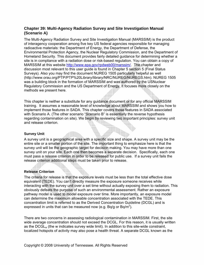
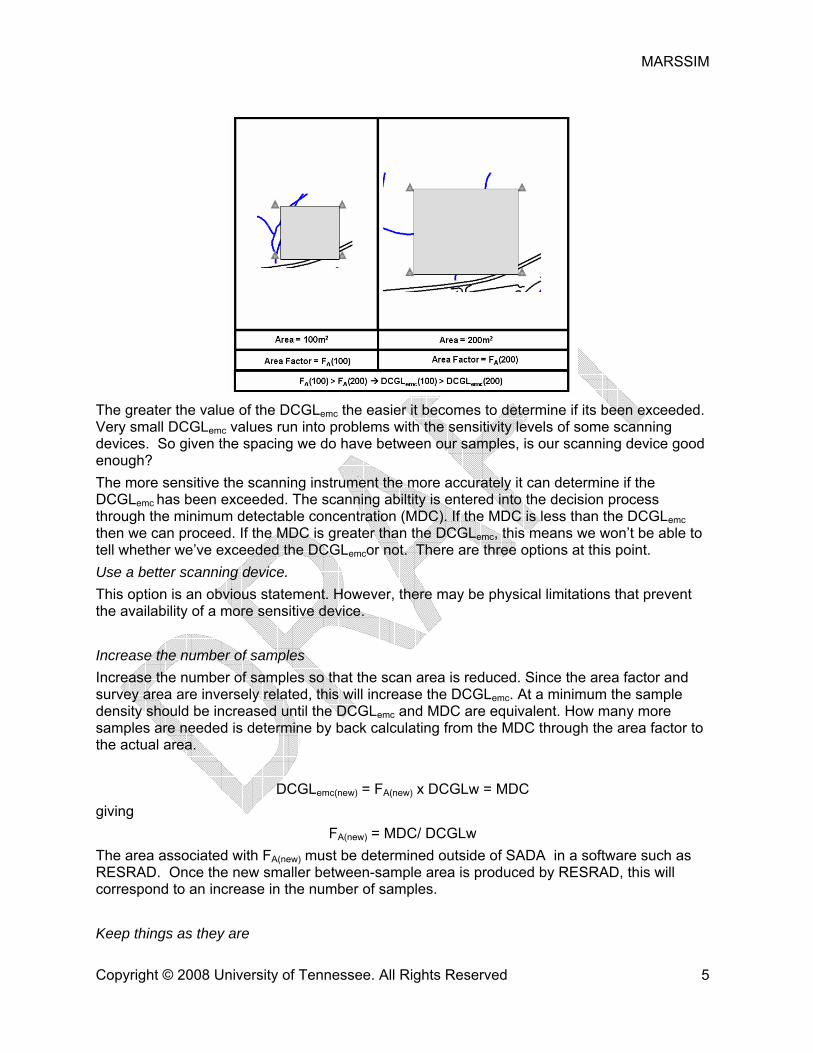
You should choose your survey units with these classifications in mind. You don’t want to divide a site into survey units in such a way that virtually every unit is a Class I. If you have areas that are likely uncontaminated you may want to spatially define you’re a sperate survey unit for this area. Consider the following figure where a contaminated area has been divided into two survey units. This now forces the classification for both to be Class I requiring both to have a higher level of sampling and analysis.
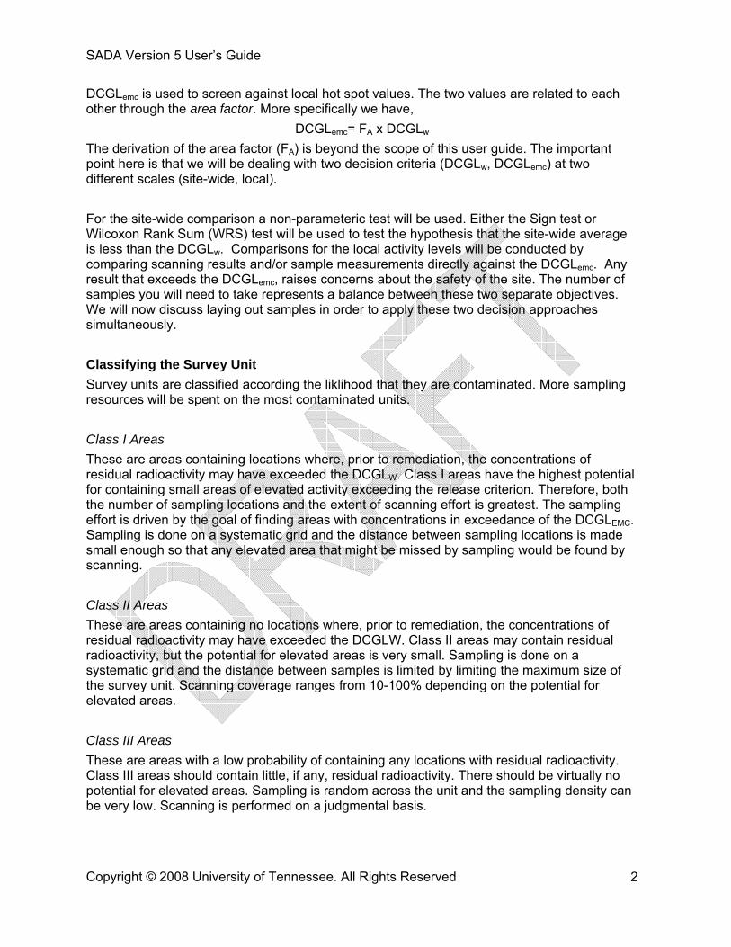
Rather you may want to divide the site into survey units that are more manageable. The following image shows the same site divided into two survey units. However this arrangement will require fewer samples as the Survey Unit B is now a Class III.
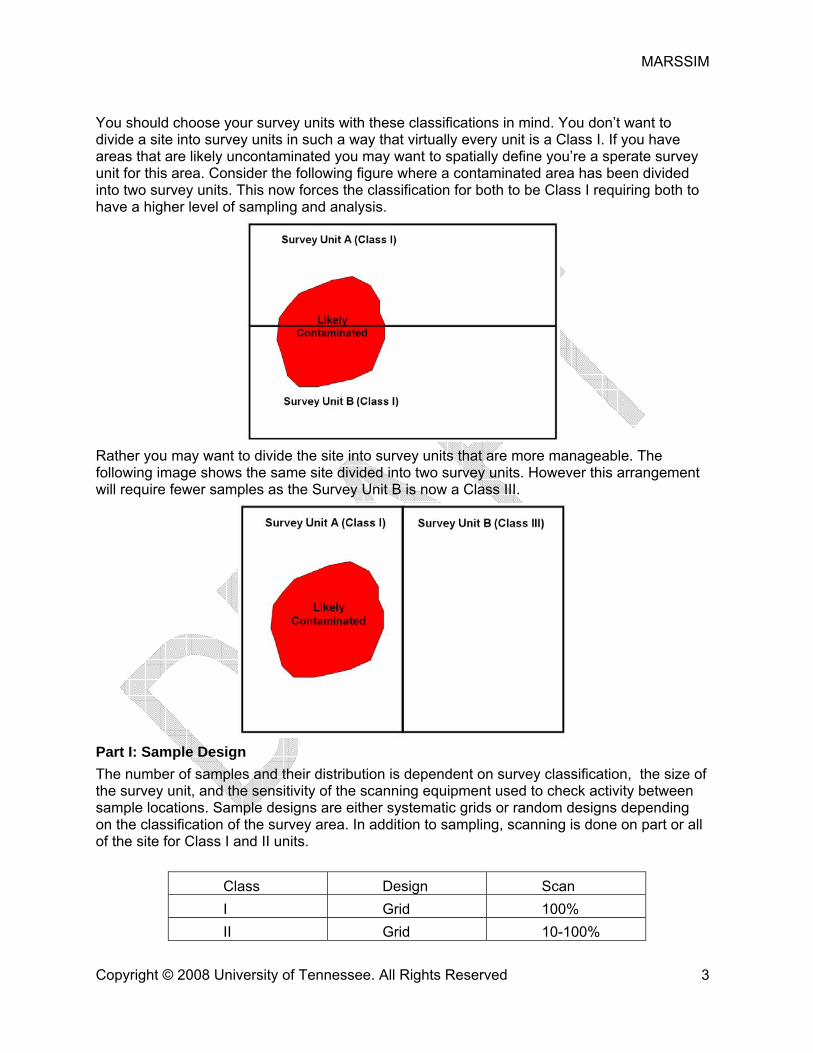
Part I: Sample Design The number of samples and their distribution is dependent on survey classification, the size of the survey unit, and the sensitivity of the scanning equipment used to check activity between sample locations. Sample designs are either systematic grids or random designs depending on the classification of the survey area. In addition to sampling, scanning is done on part or all of the site for Class I and II units.
III Random None Determine Number of Samples/Choose a Statistical Test When sampling has been completed, you will use either a Sign Test or Wilcoxon Rank Sum (WRS) test to determine if the mean concentration exceeds the DCGLw. Technically, these two methods test hypothesis about median and not the mean. If the distribution of values is roughly symmetrical then the mean and median area bout the same. If not, then MARSSIM argues that the results are still stronger than if a nonparameteric test is used (MARSSIM, sec 8.2.3). If the contaminant is present in background, then data for the contaminant is collected from a reference area and the Wilcoxon Rank Sum test is performed. If the contaminant is not present in reference samples, then the Sign Test is performed. As you recall from both the statistics chapter and the overview of sample designs chapter, it is possible to estimate apriori the number of samples to take if you are willing to make some assumptions about the data. Power curves for both the Sign and WRS test require an estimate for the data variance, the DCGLw, and tolerances for Type I and Type II errors. The result is an estimate for the number of samples to collect both in the survey unit and if necessary in the reference area. Please visit the overview of sampling designs chapter under the section on determining the number of samples for a more detailed discussion of Sign and WRS power curves. Adjust the Number of Samples for scanning (Class I/II only) For Class I areas and Class II areas, scanning the surface plays an important role in determining if contamination exists in the unit. Recall that the DCGLemc is calculated as
DCGLemc= FA x DCGLw The DCGLw is determine by an exposure pathway model. The FA can be calculated by RESRAD (http://web.ead.anl.gov/resrad/home2/). The FA depends on the area you are interested in. For us, the area is the space between the sample points. The bigger the spaces between samples, the smaller the FA (and the DCGLemc) the smaller the spaces between the samples, the higher the FA (and the DCGLemc).
The greater the value of the DCGLemc the easier it becomes to determine if its been exceeded. Very small DCGLemc values run into problems with the sensitivity levels of some scanning devices. So given the spacing we do have between our samples, is our scanning device good enough? The more sensitive the scanning instrument the more accurately it can determine if the DCGLemc has been exceeded. The scanning abiltity is entered into the decision process through the minimum detectable concentration (MDC). If the MDC is less than the DCGLemc then we can proceed. If the MDC is greater than the DCGLemc, this means we won’t be able to tell whether we’ve exceeded the DCGLemcor not. There are three options at this point. Use a better scanning device. This option is an obvious statement. However, there may be physical limitations that prevent the availability of a more sensitive device. Increase the number of samples Increase the number of samples so that the scan area is reduced. Since the area factor and survey area are inversely related, this will increase the DCGLemc. At a minimum the sample density should be increased until the DCGLemc and MDC are equivalent. How many more samples are needed is determine by back calculating from the MDC through the area factor to the actual area.
DCGLemc(new) = FA(new) x DCGLw = MDC giving
FA(new) = MDC/ DCGLw The area associated with FA(new) must be determined outside of SADA in a software such as RESRAD. Once the new smaller between-sample area is produced by RESRAD, this will correspond to an increase in the number of samples. Keep things as they are
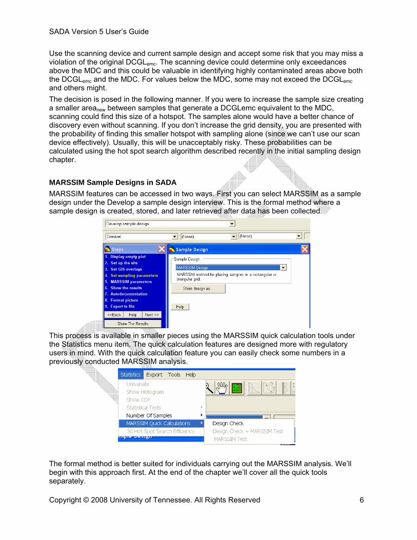
Use the scanning device and current sample design and accept some risk that you may miss a violation of the original DCGLemc. The scanning device could determine only exceedances above the MDC and this could be valuable in identifying highly contaminated areas above both the DCGLemc and the MDC. For values below the MDC, some may not exceed the DCGLemc and others might. The decision is posed in the following manner. If you were to increase the sample size creating a smaller areanew between samples that generate a DCGLemc equivalent to the MDC, scanning could find this size of a hotspot. The samples alone would have a better chance of discovery even without scanning. If you don’t increase the grid density, you are presented with the probability of finding this smaller hotspot with sampling alone (since we can’t use our scan device effectively). Usually, this will be unacceptably risky. These probabilities can be calculated using the hot spot search algorithm described recently in the initial sampling design chapter. MARSSIM Sample Designs in SADA MARSSIM features can be accessed in two ways. First you can select MARSSIM as a sample design under the Develop a sample design interview. This is the formal method where a sample design is created, stored, and later retrieved after data has been collected.
This process is available in smaller pieces using the MARSSIM quick calculation tools under the Statistics menu item. The quick calculation features are designed more with regulatory users in mind. With the quick calculation feature you can easily check some numbers in a previously conducted MARSSIM analysis.
The formal method is better suited for individuals carrying out the MARSSIM analysis. We’ll begin with this approach first. At the end of the chapter we’ll cover all the quick tools separately.
Please open the file InitialDesigns.sda. Select the Develop sample design interview and in the “Set sampling parameters” step select MARSSIM design. Click on the step MARSSIM parameters. This parameter window can exist in two states. At the top of the parameter window there is a drop-list of previously created designs and the (new) option. When you have the (new) selected, SADA understands that you want to create a new sample design and presents you with options you can customize. If you a select a previously stored design, then the customizable options are replaced with a static report of parameter values used to create the design. You cannot edit these.
At this point, we don’t have any previously stored results. Let’s divide the example into two sub-examples: Class I/II and a Class III site. The radionuclide(s) could be anything. The only place the radionuclide matters is in the calculation of the area factor and possibly the MDC. We’ll use hypothetical values for each of these. The survey unit has been delineated in the graphics window by the Actual Site Boundary polygon (see Setup the site step). Class I/II Example In the Step 1 parameter block, select “Class 1(Contamination is present)”. For our first example, we’ll assume the radionuclide is not present in background. We’ll choose the “Sign Test (No reference area needed)” under the “Step 2: Choose the statistical test” parameter block. Since the survey unit is a Class I (or II), we are also presented with the grid style option in Step 3. Select Triangular. Press the Show The Results button to proceed to more sample design parameters.
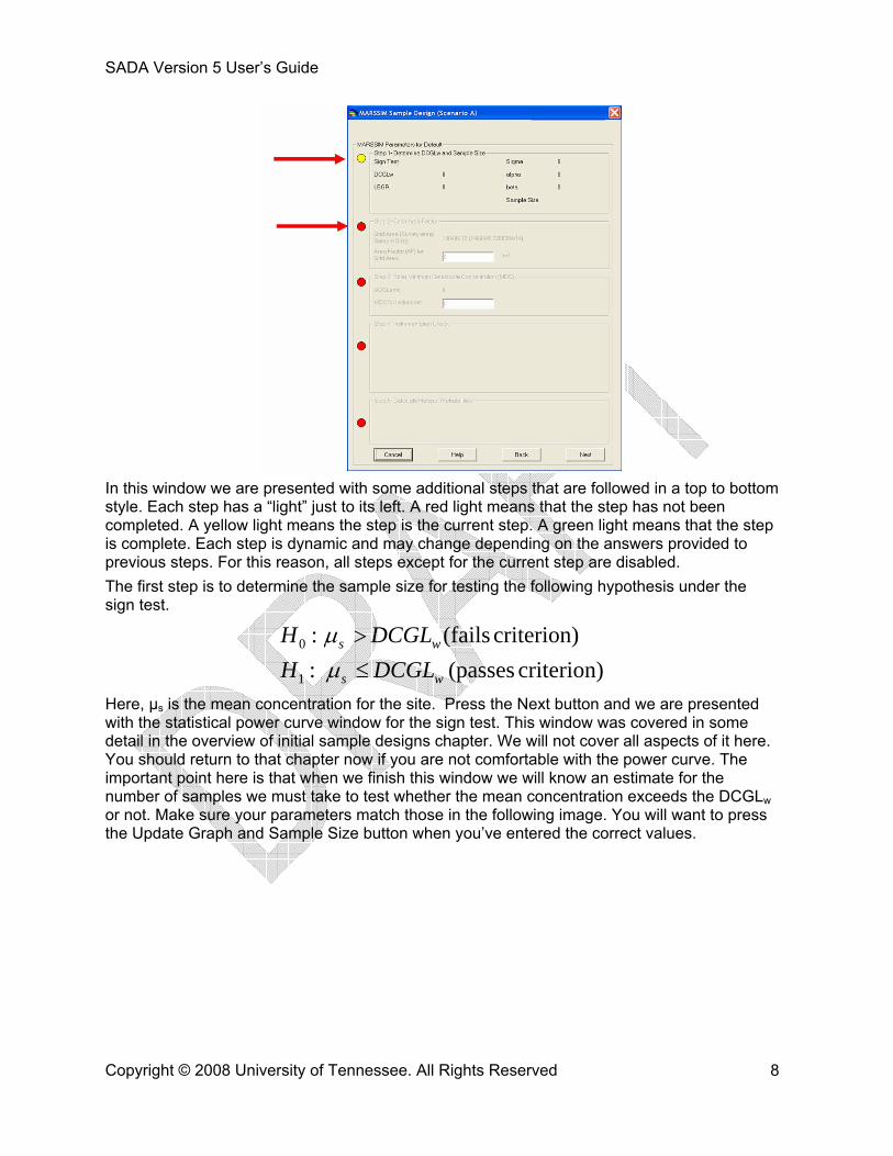
In this window we are presented with some additional steps that are followed in a top to bottom style. Each step has a “light” just to its left. A red light means that the step has not been completed. A yellow light means the step is the current step. A green light means that the step is complete. Each step is dynamic and may change depending on the answers provided to previous steps. For this reason, all steps except for the current step are disabled. The first step is to determine the sample size for testing the following hypothesis under the sign test.
criterion)(passes:criterion)(fails:
1
0
ws
ws
DCGLHDCGLH
≤>
μμ
Here, μs is the mean concentration for the site. Press the Next button and we are presented with the statistical power curve window for the sign test. This window was covered in some detail in the overview of initial sample designs chapter. We will not cover all aspects of it here. You should return to that chapter now if you are not comfortable with the power curve. The important point here is that when we finish this window we will know an estimate for the number of samples we must take to test whether the mean concentration exceeds the DCGLw or not. Make sure your parameters match those in the following image. You will want to press the Update Graph and Sample Size button when you’ve entered the correct values.
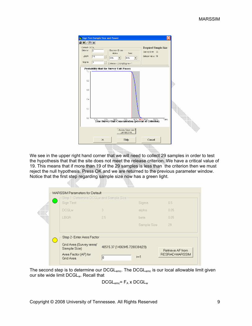
We see in the upper right hand corner that we will need to collect 29 samples in order to test the hypothesis that that the site does not meet the release criterion. We have a critical value of 19. This means that if more than 19 of the 29 samples is less than the criterion then we must reject the null hypothesis. Press OK and we are returned to the previous parameter window. Notice that the first step regarding sample size now has a green light.
The second step is to determine our DCGLemc. The DCGLemc is our local allowable limit given our site wide limit DCGLw. Recall that
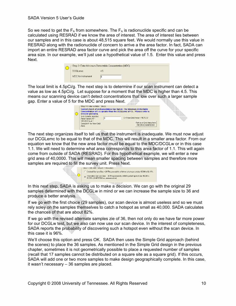
So we need to get the FA from somewhere. The FA is radionuclide specific and can be calculated using RESRAD if we know the area of interest. The area of interest lies between our samples and in this case is about 48,515 square feet. We would normally use this value in RESRAD along with the radionuclide of concern to arrive a the area factor. In fact, SADA can import an entire RESRAD area factor curve and pick the area off the curve for your specific area size. In our example, we’ll just use a hypothetical value of 1.5. Enter this value and press Next.
The local limit is 4.5pCi/g. The next step is to determine if our scan instrument can detect a value as low as 4.5pCi/g. Let suppose for a moment that the MDC is higher than 4.5. This means our scanning device can’t detect concentrations that low over such a larger sample gap. Enter a value of 5 for the MDC and press Next.
The next step organizes itself to tell us that the instrument is inadequate. We must now adjust our DCGLemc to be equal to that of the MDC. This will result in a smaller area factor. From our equation we know that the new area factor must be equal to the MDC/DCGLw or in this case 1.1. We will need to determine what area corresponds to this area factor of 1.1. This will again come from outside of SADA (RESRAD). For this hypothetical example, we will enter a new grid area of 40,0000. This will mean smaller spacing between samples and therefore more samples are required to fill the survey unit. Press Next.
In this next step, SADA is asking us to make a decision. We can go with the original 29 samples determined with the DCGLw in mind or we can increase the sample size to 36 and produce a better analysis. If we go with the first choice (29 samples), our scan device is almost useless and so we must rely soley on the samples themselves to catch a hotspot as small as 40,000. SADA calculates the chances of that are about 82%. If we go with the revised alternate samples zie of 36, then not only do we have far more power for our DCGLw test, but we also can now use our scan device. In the interest of completeness, SADA reports the probability of discovering such a hotspot even without the scan device. In this case it is 96%. We’ll choose this option and press OK. SADA then uses the Simple Grid approach (behind the scenes) to place the 36 samples. As mentioned in the Simple Grid design in the previous chapter, sometimes it is not geometrically possible to place a requested number of samples (recall that 17 samples cannot be distributed on a square site as a square grid). If this occurs, SADA will add one or two more samples to make design geographically complete. In this case, it wasn’t necessary – 36 samples are placed.
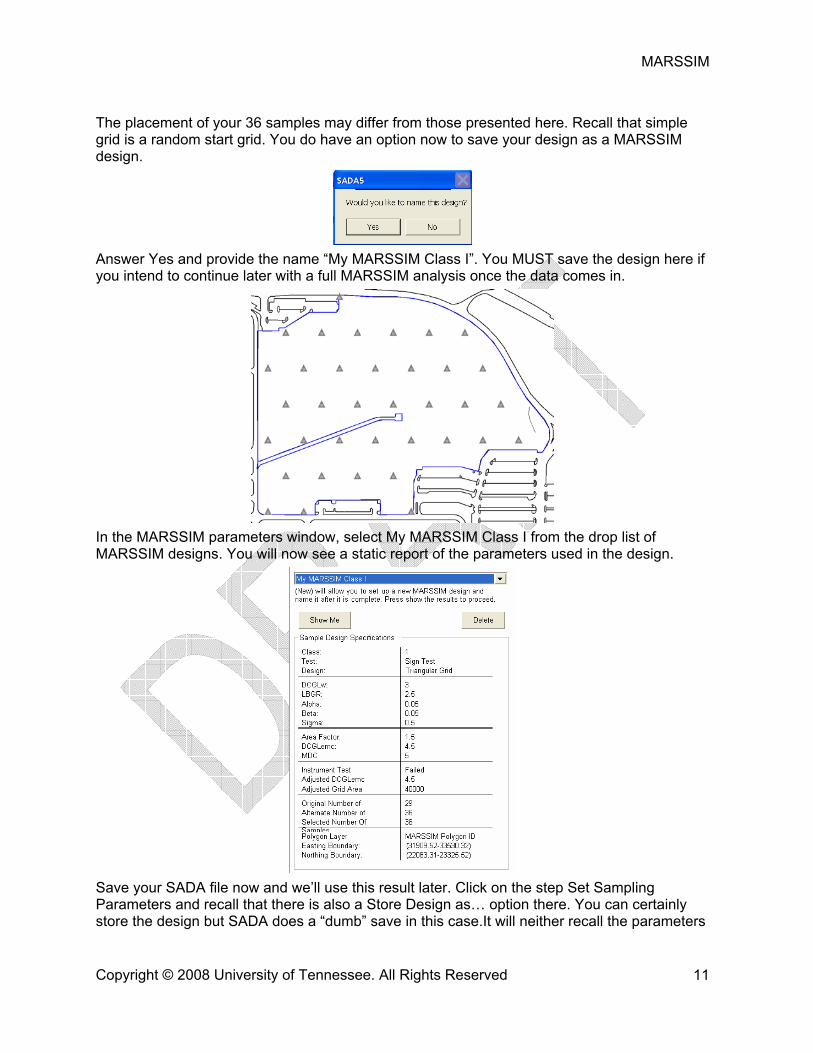
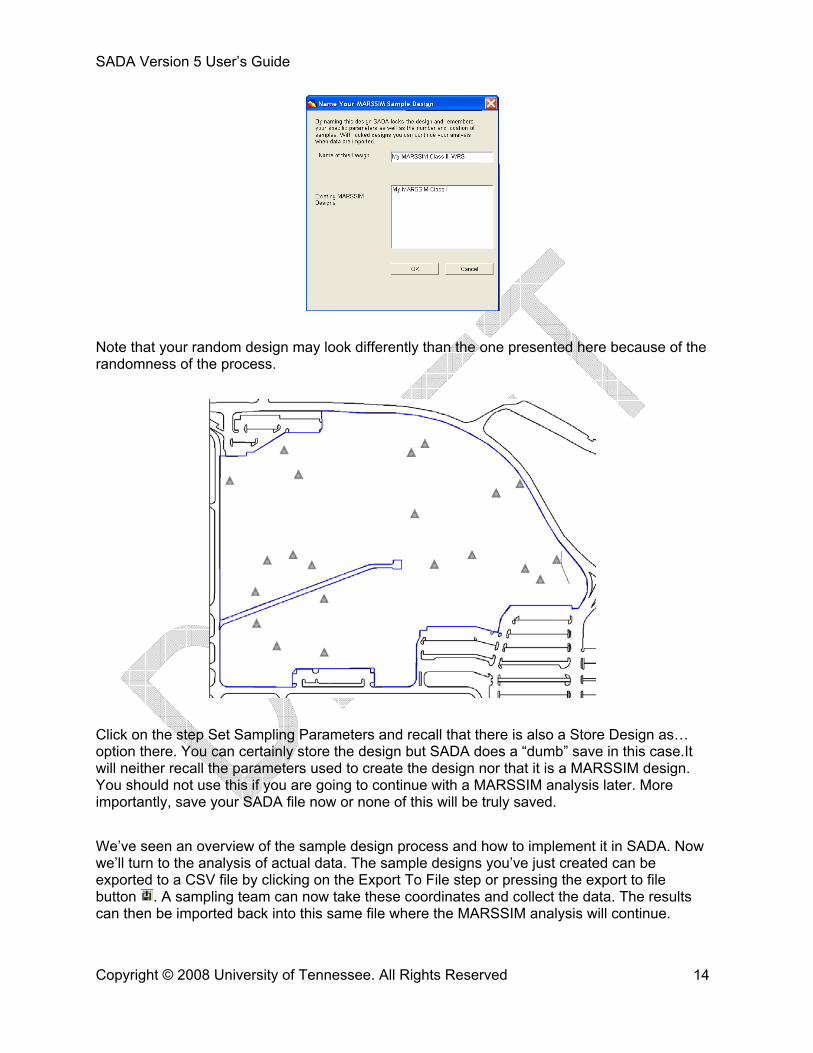
The placement of your 36 samples may differ from those presented here. Recall that simple grid is a random start grid. You do have an option now to save your design as a MARSSIM design.
Answer Yes and provide the name “My MARSSIM Class I”. You MUST save the design here if you intend to continue later with a full MARSSIM analysis once the data comes in.
In the MARSSIM parameters window, select My MARSSIM Class I from the drop list of MARSSIM designs. You will now see a static report of the parameters used in the design.
Save your SADA file now and we’ll use this result later. Click on the step Set Sampling Parameters and recall that there is also a Store Design as… option there. You can certainly store the design but SADA does a “dumb” save in this case.It will neither recall the parameters
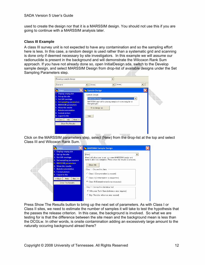
used to create the design nor that it is a MARSSIM design. You should not use this if you are going to continue with a MARSSIM analysis later. Class III Example A class III survey unit is not expected to have any contamination and so the sampling effort here is less. In this case, a random design is used rather than a systematic grid and scanning is done only if deemed necessary by site investigators. In this example we will assume our radionuclide is present in the background and will demonstrate the Wilcoxon Rank Sum approach. If you have not already done so, open InitialDesign.sda, switch to the Develop sample design, and select MARSSIM Design from drop-list of available designs under the Set Sampling Parameters step.
Click on the MARSSIM parameters step, select (New) from the drop-list at the top and select Class III and Wilcoxon Rank Sum.
Press Show The Results button to bring up the next set of parameters. As with Class I or Class II sites, we need to estimate the number of samples it will take to test the hypothesis that the passes the release criterion. In this case, the background is involved. So what we are testing for is that the difference between the site mean and the background mean is less than the DCGLw. In other words, is onsite contamination adding an excessively large amount to the naturally occuring background alread there?
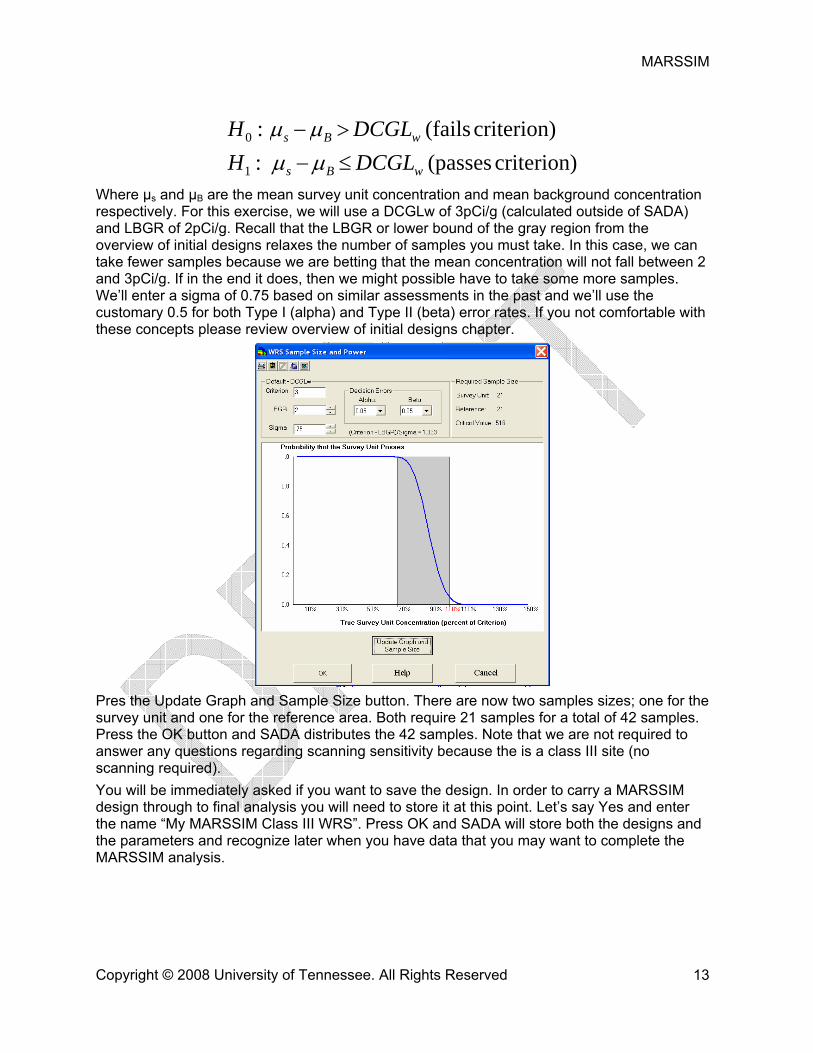
Where μs and μB are the mean survey unit concentration and mean background concentration respectively. For this exercise, we will use a DCGLw of 3pCi/g (calculated outside of SADA) and LBGR of 2pCi/g. Recall that the LBGR or lower bound of the gray region from the overview of initial designs relaxes the number of samples you must take. In this case, we can take fewer samples because we are betting that the mean concentration will not fall between 2 and 3pCi/g. If in the end it does, then we might possible have to take some more samples. We’ll enter a sigma of 0.75 based on similar assessments in the past and we’ll use the customary 0.5 for both Type I (alpha) and Type II (beta) error rates. If you not comfortable with these concepts please review overview of initial designs chapter.
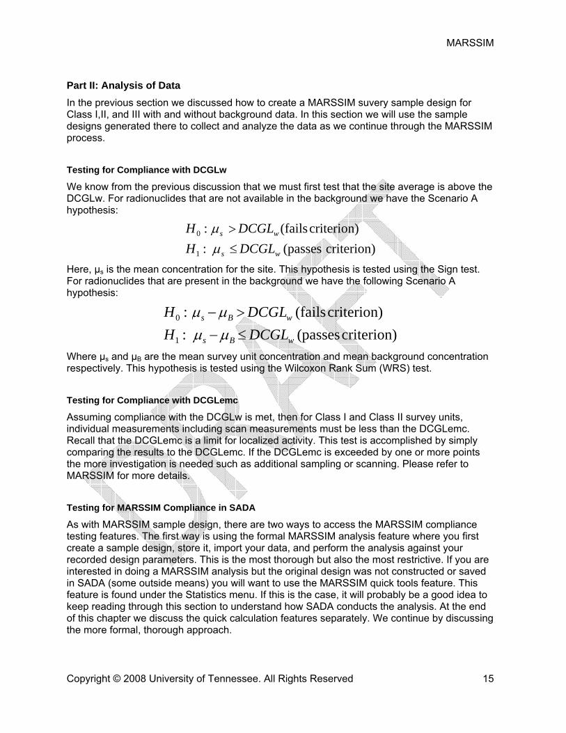
Pres the Update Graph and Sample Size button. There are now two samples sizes; one for the survey unit and one for the reference area. Both require 21 samples for a total of 42 samples. Press the OK button and SADA distributes the 42 samples. Note that we are not required to answer any questions regarding scanning sensitivity because the is a class III site (no scanning required). You will be immediately asked if you want to save the design. In order to carry a MARSSIM design through to final analysis you will need to store it at this point. Let’s say Yes and enter the name “My MARSSIM Class III WRS”. Press OK and SADA will store both the designs and the parameters and recognize later when you have data that you may want to complete the MARSSIM analysis.
Note that your random design may look differently than the one presented here because of the randomness of the process.
Click on the step Set Sampling Parameters and recall that there is also a Store Design as… option there. You can certainly store the design but SADA does a “dumb” save in this case.It will neither recall the parameters used to create the design nor that it is a MARSSIM design. You should not use this if you are going to continue with a MARSSIM analysis later. More importantly, save your SADA file now or none of this will be truly saved. We’ve seen an overview of the sample design process and how to implement it in SADA. Now we’ll turn to the analysis of actual data. The sample designs you’ve just created can be exported to a CSV file by clicking on the Export To File step or pressing the export to file button . A sampling team can now take these coordinates and collect the data. The results can then be imported back into this same file where the MARSSIM analysis will continue.
Part II: Analysis of Data In the previous section we discussed how to create a MARSSIM suvery sample design for Class I,II, and III with and without background data. In this section we will use the sample designs generated there to collect and analyze the data as we continue through the MARSSIM process. Testing for Compliance with DCGLw
We know from the previous discussion that we must first test that the site average is above the DCGLw. For radionuclides that are not available in the background we have the Scenario A hypothesis:
criterion)(passes:criterion)(fails:
1
0
ws
ws
DCGLHDCGLH
≤>
μμ
Here, μs is the mean concentration for the site. This hypothesis is tested using the Sign test. For radionuclides that are present in the background we have the following Scenario A hypothesis:
criterion)(passes:criterion)(fails:
1
0
wBs
wBs
DCGLHDCGLH
≤−>−
μμμμ
Where μs and μB are the mean survey unit concentration and mean background concentration respectively. This hypothesis is tested using the Wilcoxon Rank Sum (WRS) test. Testing for Compliance with DCGLemc
Assuming compliance with the DCGLw is met, then for Class I and Class II survey units, individual measurements including scan measurements must be less than the DCGLemc. Recall that the DCGLemc is a limit for localized activity. This test is accomplished by simply comparing the results to the DCGLemc. If the DCGLemc is exceeded by one or more points the more investigation is needed such as additional sampling or scanning. Please refer to MARSSIM for more details. Testing for MARSSIM Compliance in SADA
As with MARSSIM sample design, there are two ways to access the MARSSIM compliance testing features. The first way is using the formal MARSSIM analysis feature where you first create a sample design, store it, import your data, and perform the analysis against your recorded design parameters. This is the most thorough but also the most restrictive. If you are interested in doing a MARSSIM analysis but the original design was not constructed or saved in SADA (some outside means) you will want to use the MARSSIM quick tools feature. This feature is found under the Statistics menu. If this is the case, it will probably be a good idea to keep reading through this section to understand how SADA conducts the analysis. At the end of this chapter we discuss the quick calculation features separately. We continue by discussing the more formal, thorough approach.
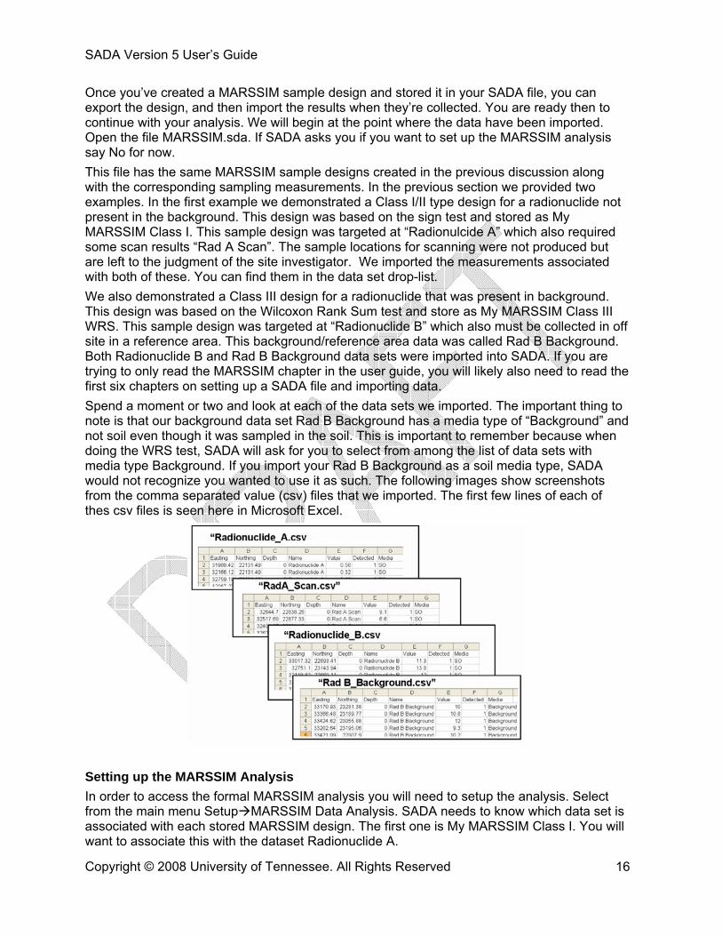
Once you’ve created a MARSSIM sample design and stored it in your SADA file, you can export the design, and then import the results when they’re collected. You are ready then to continue with your analysis. We will begin at the point where the data have been imported. Open the file MARSSIM.sda. If SADA asks you if you want to set up the MARSSIM analysis say No for now. This file has the same MARSSIM sample designs created in the previous discussion along with the corresponding sampling measurements. In the previous section we provided two examples. In the first example we demonstrated a Class I/II type design for a radionuclide not present in the background. This design was based on the sign test and stored as My MARSSIM Class I. This sample design was targeted at “Radionulcide A” which also required some scan results “Rad A Scan”. The sample locations for scanning were not produced but are left to the judgment of the site investigator. We imported the measurements associated with both of these. You can find them in the data set drop-list. We also demonstrated a Class III design for a radionuclide that was present in background. This design was based on the Wilcoxon Rank Sum test and store as My MARSSIM Class III WRS. This sample design was targeted at “Radionuclide B” which also must be collected in off site in a reference area. This background/reference area data was called Rad B Background. Both Radionuclide B and Rad B Background data sets were imported into SADA. If you are trying to only read the MARSSIM chapter in the user guide, you will likely also need to read the first six chapters on setting up a SADA file and importing data. Spend a moment or two and look at each of the data sets we imported. The important thing to note is that our background data set Rad B Background has a media type of “Background” and not soil even though it was sampled in the soil. This is important to remember because when doing the WRS test, SADA will ask for you to select from among the list of data sets with media type Background. If you import your Rad B Background as a soil media type, SADA would not recognize you wanted to use it as such. The following images show screenshots from the comma separated value (csv) files that we imported. The first few lines of each of thes csv files is seen here in Microsoft Excel.
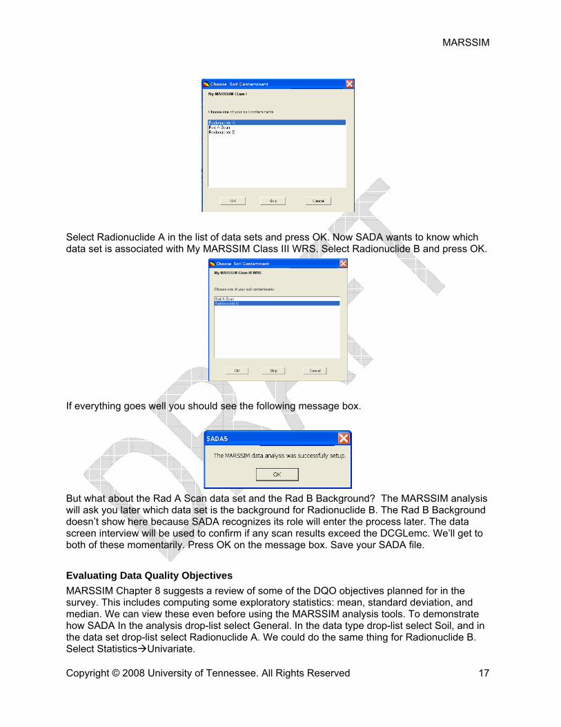
Setting up the MARSSIM Analysis In order to access the formal MARSSIM analysis you will need to setup the analysis. Select from the main menu Setup MARSSIM Data Analysis. SADA needs to know which data set is associated with each stored MARSSIM design. The first one is My MARSSIM Class I. You will want to associate this with the dataset Radionuclide A.
Select Radionuclide A in the list of data sets and press OK. Now SADA wants to know which data set is associated with My MARSSIM Class III WRS. Select Radionuclide B and press OK.
If everything goes well you should see the following message box.
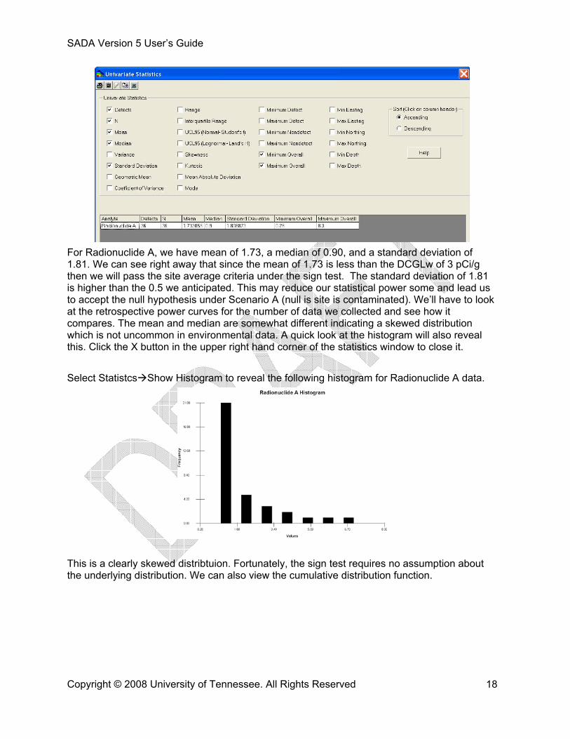
But what about the Rad A Scan data set and the Rad B Background? The MARSSIM analysis will ask you later which data set is the background for Radionuclide B. The Rad B Background doesn’t show here because SADA recognizes its role will enter the process later. The data screen interview will be used to confirm if any scan results exceed the DCGLemc. We’ll get to both of these momentarily. Press OK on the message box. Save your SADA file. Evaluating Data Quality Objectives MARSSIM Chapter 8 suggests a review of some of the DQO objectives planned for in the survey. This includes computing some exploratory statistics: mean, standard deviation, and median. We can view these even before using the MARSSIM analysis tools. To demonstrate how SADA In the analysis drop-list select General. In the data type drop-list select Soil, and in the data set drop-list select Radionuclide A. We could do the same thing for Radionuclide B. Select Statistics Univariate.
For Radionuclide A, we have mean of 1.73, a median of 0.90, and a standard deviation of 1.81. We can see right away that since the mean of 1.73 is less than the DCGLw of 3 pCi/g then we will pass the site average criteria under the sign test. The standard deviation of 1.81 is higher than the 0.5 we anticipated. This may reduce our statistical power some and lead us to accept the null hypothesis under Scenario A (null is site is contaminated). We’ll have to look at the retrospective power curves for the number of data we collected and see how it compares. The mean and median are somewhat different indicating a skewed distribution which is not uncommon in environmental data. A quick look at the histogram will also reveal this. Click the X button in the upper right hand corner of the statistics window to close it. Select Statistcs Show Histogram to reveal the following histogram for Radionuclide A data.
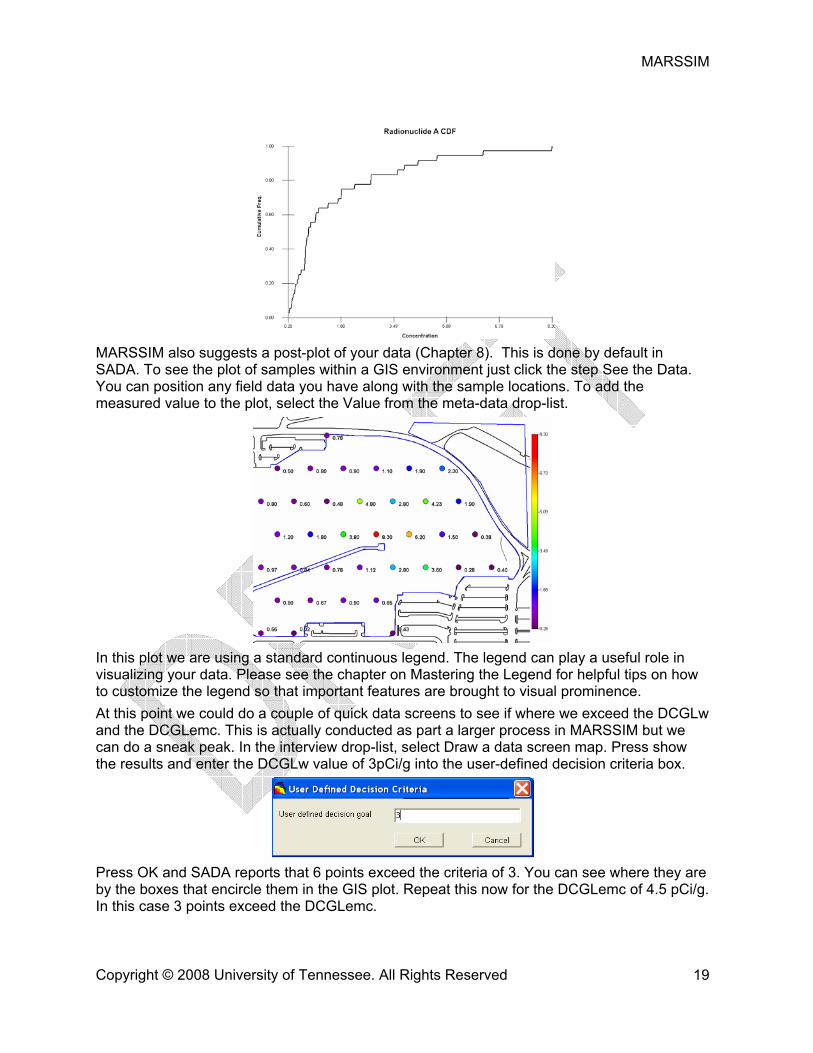
This is a clearly skewed distribtuion. Fortunately, the sign test requires no assumption about the underlying distribution. We can also view the cumulative distribution function.
MARSSIM also suggests a post-plot of your data (Chapter 8). This is done by default in SADA. To see the plot of samples within a GIS environment just click the step See the Data. You can position any field data you have along with the sample locations. To add the measured value to the plot, select the Value from the meta-data drop-list.
In this plot we are using a standard continuous legend. The legend can play a useful role in visualizing your data. Please see the chapter on Mastering the Legend for helpful tips on how to customize the legend so that important features are brought to visual prominence. At this point we could do a couple of quick data screens to see if where we exceed the DCGLw and the DCGLemc. This is actually conducted as part a larger process in MARSSIM but we can do a sneak peak. In the interview drop-list, select Draw a data screen map. Press show the results and enter the DCGLw value of 3pCi/g into the user-defined decision criteria box.
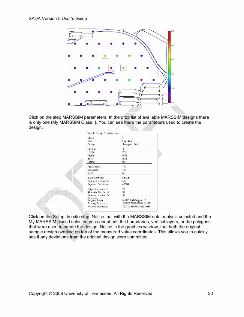
Press OK and SADA reports that 6 points exceed the criteria of 3. You can see where they are by the boxes that encircle them in the GIS plot. Repeat this now for the DCGLemc of 4.5 pCi/g. In this case 3 points exceed the DCGLemc.
Click on the step MARSSIM parameters. In the drop list of available MARSSIM designs there is only one (My MARSSIM Class I). You can see there the parameters used to create the design.
Click on the Setup the site step. Notice that with the MARSSIM data analysis selected and the My MARSSIM class I selected you cannot edit the boundaries, vertical layers, or the polygons that were used to create the design. Notice in the graphics window, that both the original sample design overlaid on top of the measured value coordinates. This allows you to quickly see if any deviations from the original design were committed.
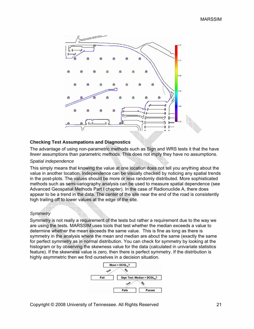
Checking Test Assumpations and Diagnostics The advantage of using non-parametric methods such as Sign and WRS tests it that the have fewer assumptions than parametric methods. This does not imply they have no assumptions. Spatial independence This simply means that knowing the value at one location does not tell you anything about the value in another location. Independence can be visually checked by noticing any spatial trends in the post-plots. The values should be more or less randomly distributed. More sophisticated methods such as semi-variography analysis can be used to measure spatial dependence (see Advanced Geospatial Methods Part I chapter). In the case of Radionuclide A, there does appear to be a trend in the data. The center of the site near the end of the road is consistently high trailing off to lower values at the edge of the site. Symmetry Symmetry is not really a requirement of the tests but rather a requirement due to the way we are using the tests. MARSSIM uses tools that test whether the median exceeds a value to determine whether the mean exceeds the same value. This is fine as long as there is symmetry in the analysis where the mean and median are about the same (exactly the same for perfect symmetry as in normal distribution. You can check for symmetry by looking at the histogram or by observing the skewness value for the data (calculated in univariate statistics feature). If the skewness value is zero, then there is perfect symmetry. If the distribution is highly asymmetric then we find ourselves in a decision situation.
If the mean is greater than the DCGLw, then its simple; the site fails. If the mean is less than the DCGLw we are forced to slightly change our question in order to use the Sign (or WRS) test. If we use the Sign or WRS test we are now asking whether the median exceeds the DCGL. The following outcomes are possible.
Fails Passes Symmetric OK OK Median > Mean May unnecessarily remediate. OK Median < Mean OK May erroneously release the site In those cases where the median is less than the mean and the Sign test passes (rejects null), then investigators should be careful and possible think about a transformation of the data. You can for example perform a normal score transform which converts any distribution into a normal distribution (GSLIB, 1992, p.209) which would guarantee symmetry. Data Variance Samples sizes were generated initially based on an assumption about the standard deviation. One should compare the estimated and actual standard deviation to determine how the test may be affected. If the sample standard deviation is less than the estimated deviation then you should have enough statistical power in the test. If the sample standard deviation is greater than the deviation you estimated during the design, then depending on the median value you may or may not have enough statistical power. Retrospective Power Curve When you created your sample design the number of samples was computed such that your power curve met an alpha and beta level for a DCGlw and associated LBGR. This was based on the standard deviation as well. Now that we have collected the data, we know more about the standard deviation and can compare the powercurve with the more recent value. However instead of using the number of samples required for the test, we will use the actual number of samples taken. This might be more for Class I/II units where scanning requirements demanded more samples. Determining Compliance Compliance is determined by the following tables (based on MARSSIM Chapter 8). Sign Test (no background) Survey Result Conclusion All values less than DCGLw Survey unit meets release criterion Average greater than DCGLw Survey unit does not meet release criterion Any measurement greater than DCGLw and average is less thean DCGLw
Conduct sign test and elevated measurement comparison. If the sign test is passed, then the site
meets the release criterion. If the sign test fails, the site does not
meet the criterion. If the elevated measurement comparison
fails, then passing the sign test should be taken cautiously.
Wilcoxon Rank Sum Test (with background) Survey Result Conclusion Difference between largest survey unit measurement and smallest reference area measurement is less than DCGLw
Survey unit meets release criterion
Difference of survey unit average and reference area is greater than the DCGLw
Survey unit does not meet release criterion
Difference between any survey unit measurement and any reference area measurement greater than DCGLw and the difference of survey unit average and reference area average is less than DCGLw
Conduct WRS test and elevated measurement comparison If the WRS test is passed, then the site
meets the release criterion. If the WRS test fails, the site does not
meet the criterion. If the elevated measurement comparison
fails, then passing the WRS test should be taken cautiously.
We will now show to test for compliance in SADA for the previously created Class I/II and Class III example designs. A Class I/II Example Switch from the General Analysis to the MARSSIM Data Analysis. The only analysis permitted is to perform an MARSSIM Analysis (Scenario A).
Press Show the Results and the following window is presented.
SADA conducts the test for the DCGLw and DCLGemc (measured values only) in six instantaneous steps. Before we discuss the steps, notice the Retrospective Power Curve for Radionuclide A graph on the right side. This graph shows the original power curve for 29 samples in blue. Recall though that we needed to increase the number of samples to 36 in order to meet the DCGLemc scanning requirements. We did collect 36 samples but the standard deviation was not 0.5 as we estimated. In fact it was somewhat higher (1.81). Fortunately the additional samples taken to support the DCGLemc actually helped the DCGLw analysis as well be off-setting the higher standard deviation. For this reason, the power curves almost overlap. Step 1: Enough Samples? This step is not necessarily in either NUREG 1505 or MARSSIM (NUREG 1575). In this step we recompute the number of samples required using the new standard deviation and a relaxed beta value of 0.5. Beta refers to the likelihood that you may accept the null hypothesis (site is contaminated) when it isn’t true. This step will generate a much smaller number of samples than the original sample design. In a sense it provides a lower bound on the number of samples through relaxing the constraint against incorrectly accepting the null (site is contaminated). The spirit of this step is to prevent one from having to return to the site and sample further if the standard deviation in fact was much higher. This step is really only relevant if you fail it. This means that even with a relaxed beta you didn’t take enough samples. If you pass this step, you know you at least made it over a very low-bar sampling requirement. In this case we pass it because we took 36 samples and the low-bar requirement is 8 samples. Of course if you did only take 8 samples you are in considerable danger of saying the site is contaminated when it is not. You can actually revisit the power curve with your known standard deviation by choosing Statistics Number of Samples Sign Test (or WRS Test). This will tell you how many samples you really needed. You can also observe the retrospective power curve to see if enough were taken.
Step 2: How many samples exceeded the DCGLw? This is informing us about how many times the DCGLw was exceeded. If no measured values exceeds the DCGLw, then the site meets the release criterion. You don’t need to examine any of the remaining steps. They are presented only for completeness. In this case we had six samples in excess. This does not mean the site fails. It only means that we will need to continue through the steps by looking at the average concentration next.
Step 3: What is the survey mean concentration? This is really the first opportunity where the site could fail the release criterion. If the mean concentration exceeds the DCGLw there is no point in continuing. The site fails. The remaining steps will be presented by they are only provided in the interest of completeness. If the mean is less than the DCGLw, then we don’t necessarily pass either we just need to perform the Sign test. In this case we did have some values exceeding the DCGLw (Step 2) so even though our mean was less than the DCGLw we are required to do the sign test.
Step 4: Sign Test for DCGLw This is really where we get a final answer on the pass/fail regarding the DCGLw. In this case if we pass, this means that the hypothesis is rejected and that the site is classified as clean. If we fail, then we have problems. You might recall from the sample design phase that a critical value of 19 was estimated. So if we had 19 samples fall below the DCGLw then the site would pass. Because of the larger standard deviation this critical value was bumped to 23.to retain an alpha and beta of 0.05. Thirty measurements actually fell below the DCGLw.
This step is only necessary if Step 4 was necessary (it was in this example). If are put into the position of using the Sign test then you are also in the position of screening against the DCLGemc. In this step, we compare all measured values against the DCGLemc. But this is only half the story for Class I/II sites. Those sites must also compare the scan results against the DCGLemc. We’ll do that shortly as an example. It wouldn’t necessariliy be required though because we already fail here with 3 of the 36 samples exceeding the DCGLemc. Step 5 failure does not mean failure to meet the release criterion. It is essentially a warning that caveats the results of the sign test (MARSSIM, section 8.5.1).
Step 6: Did the Site Pass? In this example, the site does pass the release criterion because it passed the sign test. The result should be cautiously accepted because individual measurements failed the elevated measurement comparison.
Press the OK button. Compare Scan Data Against DCGLemc We already know tha some of the lab samples have exceeded the DCGLemc so more actions may need to be taken. However, we demonstrate here how to easily compare the scan results against the DCGLemc as well. An spatially informative way is to use the interview “Draw a data screen map”. Unfortunately at this time, we can’t access this interview under a MARSSIM analysis. We need to switch quickly back to the General analysis then select Rad A Scan and draw a data screen map interview.
Recall that under the General analysis you can have a single decision criteria or a depth variable criteria. Click on the Set decision threshold type step and just confirm that we have single decision criteria selected. Press Show the Results and enter or DCGLemc value of 4.5 into the user defined criteria.
Press Ok and SADA reports that 6 scan values exceed the DCGLemc. They are identified by boxes around each point.
It is clear from both the DCGLw and DCLGemc evaluations that this site will require some additional investigation before release to the public. At this point you might bring some of the geospatial models to bear in order to better refine the local elevated area and perhaps inform a remedial design. After the WRS example we’ll demonstrate how you can do this. WRS Example Now we’ll take a look at Radionuclide B under a Class III scenario. For this example we assumed B was present in the background as well and so a WRS test was necessary. Let’s switch back to the General Analysis and select Radionuclide B.
At this point you would want to do some of the same DQO checks and verification of assumptions we previously talked about and demonstrated with the Radionuclide A. We won’t repeat those here. Take a look at both the Radionuclide B plots and the Rad B Background data (select background instead of soil). They are presented side by side here.
If your background data does not have geographic coordinates, you can still use it. Simply create fake coordinates to get it past SADA’s data requirements. The coordinates won’t enter into the MARSSIM analysis. Select Soil again and choose Radionuclide B. Switch the analysis to MARSSIM data analysis. Click on the MARSSIM parameters step to see the details of our WRS Class 3 sample design.
The next step is to specify the background data. Click on this step now and select Rad B Background from the drop-list of available background data sets.
Press OK. Press Show the results and the MARSSIM analysis window will reappear. We’ll investigate these results step by step. Step 1: Compare Sample Size to Minimum Sample Size. This step is not necessarily in either NUREG 1505 or MARSSIM (NUREG 1575). In this step we recompute the number of samples required using the new standard deviation and a relaxed beta value of 0.5. Beta refers to the likelihood that you may accept the null hypothesis (site is contaminated) when it isn’t true. This step will generate a much smaller number of samples than the original sample design. In a sense it provides a lower bound on the number of samples through relaxing the constraint against incorrectly accepting the null (site is contaminated). The spirit of this step is to prevent one from having to return to the site and sample further if the standard deviation in fact was much higher. This step is really only relevant if you fail it. This means that even with a relaxed beta you didn’t take enough samples. If you pass this step, you know you at least made it over a very low-bar sampling requirement. In this case we pass it because we took 21 samples and the low-bar requirement is 6 samples. Of course if you did only take 6 samples you are in considerable danger of saying the site is contaminated when it is not. You can actually revisit the power curve with your known standard deviation by choosing Statistics Number of Samples WRS Test. This will tell you how many samples you really needed. You can also observe the retrospective power curve to see if enough were taken.
Step 2: Step 2: Compare Site Measurements Versus DCGLw When background is involved, we look at the differences between site and reference area rather than measured values themselves. In this case we want to examine the worst case scenario in some sense. If we take the highest survey value and the smallest background value, is there difference more than the DCGLw? If it isn’t then we know the site passes criterion because all other possible differences will certainly be below the DCGLw meaning that the average will also be less. If we pass then the site does meet the release criterion and the remaining steps are provided only in the interest of completeness. If we fail, then we may or may not fail to meet the release criterion. We’ll need to continue through the steps to find out. In this case, we did fail. We will need to continue to step 3.
Step 3: Compare mean difference between survey and background This is the first step in which we can unequivocably fail. If we the mean of the survey data minus the mean of the background data is greater than the DCGLw, then we fail to meet the release criterion and no further steps are necessary. If we pass, then we need to continue with the remaining steps.
Step 4: Conduct statistical test versus DCGLw If you have made it this far, then this step will provide the final answer in some sense. If the site passes the WRS test (reject null hypothesis that site is contaminated) then the release criterion is met. Otherwise, the release criterion is failed. In this example, we passed the test. The critical value of 516 was exceeded by 651 combinations of survey and background data differences falling below the DCGLw.
Step 5: Class III compare all measurements to 10% of DCGLw The following step is not necessarily part of the MARSSIM guidance. It is a step that affords a little more confidence in the decision by comparing all survey measurements against a small percentage (10%) of the DCGLw. Failing this does not imply the site fails the release criterion. Passing it however affords a greater case for release of the site.
Connecting Geospatial Decision Analysis and MARSSIM SADA provides a number of tools that can further support or even extend a MARSSIM analysis particularly when there is a failure when comparing against DCGLemc. Chapters 28-37 discuss geospatial decision support including determining the area of concern (in this case
a local elevated area), placement of additional samples, and rudimentary cost-benefit analysis. In this section we will point out how SADA can be used to bound local areas of elevated activity. If you are interested in exploring these further please visit the aforementioned chapters. Determining the Area of the Elevated Zone for determining Area Factor (simple way). SADA can help you determine the area of the elevated activity in direct accordance with MARSSIM. In section 8.5.1 we have the following regarding the actual area of elevated concentration. “The area of elevated activity is generally bordered by concentration measurements below the DCGLw. An individual elevated measurement on a systematic grid could conceivably represent an area four times as large as the systematic grid area used to define the DCGLEMc. This is the area bounded by the nearest neighbors of the elevated measurement location.” In this spirit SADA provides a simple tool for determining the actual area of elevated concentration. In the Set up step, simply use the polygon drawing tools to trace around the elevated points using those points less than the DCGLw to guide you. When you are done, select Tools Area of polygons. SADA will generate a report that gives the area of every polygon in place.
Determining the Area of the Elevated Zone for determining Area Factor (geospatial way). It is possible to use the full geospatial decision models in SADA to determine the area of the elevated zone. One can even develop uncertainty bands on the elevated zone. In the following image, we have the same elevated zone identified by a dark boundary line. At the center is a gray region that is most likely elevated. The green boundary indicates uncertainty abou where the boundary line may fall.
SADA can also produce area estimates that can include or not include the uncertain boundary regions. Placing Additional Samples SADA provides a couple of methods for determining where to place new samples that are relevant to a MARSSIM investigation.
1. Threshold radial – if you have only one or two exceedances, use the threshold radial method to bound the offending samples to determine if an elevated zone really exists.
2. High value design – use this method to place new samples in the area identified by geospatial modeling as a high activity area.
3. Boundary design – use this method to place new samples so that the exact location of the boundary line between elevated and unelevated zone can be better determined. This is useful particularly if you are considering dividing the unit into different survey units.
In the example below, we’ve used a high value design to optimally locate 4 new samples in the high activity area.
MARSSIM Quick Tools This formal process can be divided into smaller pieces more readily accessible. To use these you don’t have to have the MARSSIM analysis setup. You may not even need any data imported into SADA if you are just doing a design check. These tools can be found under the Statistics MARSSIM Quick Calculations. Quick Design Check This tool simply calculates the number of samples a MARSSIM test would require. It does not place them. This is useful to quickly check that an investigator has used an appropriate number of samples. Select Statistics MARSSIM Quick Calculations Design Check. This brings up the first of two parameters sets that you will already be familiar with. You’ll pick the class, the grid type (if needed), and set the statistical test just as before. The last parameter block regards the area of your survey unit. You can simply enter in the survey unit area if you have it calculated elsewhere. If actually have the survey unit setup in SADA you can use that as well. Click on “use provided area”.
Press the Next>> button and you will be presented with exactly the same parameters you’ve seen before. We won’t repeat them here. Enter values of your choosing into each of the steps. Step one will give you the number of samples for the test. The remaining steps will consider any scanning needs as before.
Press the OK button and the tool is dismissed. Quick MARSSIM Test This feature allows you to perform a MARSSIM test without having previously stored a MARSSIM design in SADA and/or setup the MARSSIM analysis. Select Statistics MARSSIM Quick Calculations MARSSIM Test.
Enter all the information about the design here including the number of required samples. You can enter as anything you wish. Press the OK button.
You will need to select a data set to run the MARSSIM test on. Therefore you will need to have imported the data before hand. Select Radionuclide A and press OK. You will be presented with the usual MARSSIM analysis window.
Quick Design Check + MARSSIM Test This really just combines the last two features into one continuous stream. The only difference will be that the first screen encountered with the MARSSIM Test is unnecessary.