CHAPTER 4 ANALYSIS OF WATER QUALITY AND POLLUTION …

CHAPTER 4

ANALYSIS OF WATER QUALITY AND POLLUTION LOADING

IN THE BURIGANGA RIVER

4.1 Introduction

In the course of the present research a total of seven months were utilised for extensive

field work to collect water samples both from river receptor points and wastewater

discharge points. The field work was performed in two different phases to examine the

temporal and the spatial variations of selected water quality parameters. Dry season was

chosen for the first phase of field work and the samples were collected between the

months of November 2008 and February 2009. The second phase of field work was

conducted during the wet season, which was between the months of August and October

2009. Throughout the field work in situ measurements and laboratory analysis were

carried out to determine the chemical composition of water samples. Further, the

characteristics of ten physicochemical parameters (as mentioned in section 3.1) for both

river and waste water were statistically analysed and compared with the DOE standards in

order to identify the status of water quality of the Buriganga River. Based on these

primary data this chapter provides a detailed and an up to date evaluation on the state of

water quality and pollution in the Buriganga River.

4.2 Methodology

4.2.1 Sampling locations

Along the Buriganga River from upstream (Bosila bridge) to downstream (Hariharpara)

five locations (receptor points) were selected in order to collect the water samples from

the river. The sampling stations were chosen at a distance of minimum 0.5 km to a

maximum of 5.5 km longitudinally away from the wastewater discharge points to

understand the state of ambient water quality in the river. Samples were also collected

from three main pollution discharge routes (discharge points) as identified in section

55

3.2.3. The locations of the sampling points have been illustrated in Figure 4.1. The

latitude and the longitude of the sampling points (Table 4.1) were recorded with Garmin

GPS 76 logger in order to have the consistency of sampling sites for subsequent sampling

events. The water samples were collected from a depth of 1 (one) meter below the

surface. The samples were gathered from eight different locations (including receptor and

discharge points) in each season (dry and wet) on five different events (as listed in Table

4.2). Hence, a total of 80 water samples were collected for analysing ten water quality

parameters.

4.2.2 In situ measurements and chemical analysis

Temperature, DO, pH and ECw were measured in every sampling event using the portable

YSI 6600 Multi probe field analyser. The multi probe device was calibrated before each

use as described in the user manual (YSI 2002).

Water samples were collected using a long-handled (about 1.5 m) grab sampler from each

site and were immediately stored in ice before being transported to the laboratory for

chemical analysis (tests for BOD5, COD, phosphate phosphorus and ammonia nitrogen

were performed at the Environmental Chemistry Lab of the Independent University in

Bangladesh and the tests for Pb and Cr were performed at the Environmental Engineering

Lab of BUET in Bangladesh). When the analysis of the samples could not be completed

within 24 hrs, the samples were preserved with 0.8 ml sulphuric acid (H2SO4) for each

litre of sample and then stored at 4 0C as recommended by Chapman and Kimstach

(1992).

The chemical analyses in the laboratories were performed following the standard

procedures of APHA (1998). The equipments and their detection limits are given in Table

4.3.

56

2 km

5

4

3

2

1

C

B

A

N

(a)

(b)

Figure 4.1. (a) A satellite map showing water sampling points in Buriganga River

(Adapted and modified from: Google Earth 2010)

(b) A schematic diagram (with chainage distance) of the sampling points

57

Table 4.1. Geographical position (latitude and longitude) of the sampling points

Sampling points

Locations Buriganga chainage (km)

Latitude and Longitude

Remarks

1 Bosila bridge 0.0 N 23.7433 0

E 90.3458 0River water

2 Kholamora 2.5 N 23.7191 0


3 Muslimbag 6.0 N 23.7066 0


4 Faridabad 10.0 N 23.6912 0


5 Hariharpara 17.0 N 23.6326 0


A Rayerbazar sluice gate

0.5 N 23.7415 0

E 90.3514 0Wastewater discharge point

B Shahidnagar drainage outlet

6.5 N 23.7102 0


C PSTP effluent outfall 12.0 N 23.6745 0


Table 4.2. Sampling dates and weather condition

Sampling

days

Dates Season Weather condition

1 12/12/2008 Dry Cold, Clear



4 16/02/2009 Dry Fine

5 14/03/2009 Dry Fine

6 08/08/2009 Wet Hot, Clear

7 22/08/2009 Wet Hot, Cloudy

8 24/09/2009 Wet Hot, Clear

9 8/10/2009 Wet Fine

10 27/10/2009 Wet Fine

58

Table 4.3. Test methods with detection limits and special equipments for

chemical water quality parameters

Parameters Tests Detection limits Required special equipments

BOD5 Dilution method

No limit BOD bottle

COD Open Reflux method (two procedures for different detection limits)

0-50 mg/L > 50 mg/L

Reflux apparatus

Pb Dithizone method

0-0.30 mg/L Digital reactor block (HACH DR-2000)

Cr (VI) Direct Air-Acetylene Flame method

No limit Atomic Absorption Spectrophotometer (Shimadzu AA-6800)

PO4-P Amino Acid method

0-30 mg/L Digital reactor block (HACH DR-2000)

NH3-N Ammonia-Selective Electrode method

0.03-1400 mg/L pH meter with expanded millivolt scale (Omega PHH-65A)

4.2.3 Flow measurements for wastewater

The wastewater flow rates from the discharge points were measured by velocity-area

method (Chitale 1974; USEPA 1997; Gore 2007). This technique comprises measuring

the mean velocity and the flow area, and then computing the discharge from the

continuity equation as:

Q = A* V (4.1)

where, Q = wastewater flow rate

A = cross-sectional area of the flowing wastewater

V = average velocity of the wastewater

The cross-sectional area was determined by the product of width and depth of the flowing

wastewater which were discharged through open rectangular channels. The velocities of

wastewater at the discharge points were measured by applying the float method (USEPA

1997; Cassidy 2003) during ten different sampling events. To perform this method, time

was recorded with a stop watch for a buoyant object (half filled bottles) to float a

59

specified distance along the flow of the wastewater. The velocities in each sampling event

were calculated as the travel distance of the object divided by the recorded travel time

(this procedure was repeated three times in each occasion and the average velocity was

recorded).

4.2.4 Estimation of pollution load

Estimation of pollution load (amount of pollution) from the wastewater discharge points

is an essential precursor to develop alternative and effective pollution abatement policies.

For the purpose of the alternative pollution abatement policy analysis, the wastewater

quality parameter of interest in this research was focused on BOD5 loading and its

interaction with DO levels in river water. The theoretical relationship between these two

parameters was established mathematically from the oxygen sag curve (Figure 2.1) as

described in Streeter and Phelps (1925). In this research, the pollution load was measured

for BOD5 using the averaging estimation approach (Dolan et al. 1981; Ferguson 1987;

Preston et al. 1989; Letcher et al. 1999) as per following equation:

Le = (4.2) 1

1/n

i

n Ci=

⎛ ⎞⎜ ⎟⎝ ⎠

∑1

1/n

i

n Qi=

⎛ ⎞⎜ ⎟⎝ ⎠

∑

where,

Le = Estimated pollution load

n = Number of samples taken during the study period

Ci = Concentration of the pollutant at the time of sampling

Qi = Flow rate of wastewater at the time of sampling

4.2.5 Statistical analysis

One way analysis of variance (ANOVA) involving two factors (sampling locations and

seasons) without replication was performed employing the statistical package OpenStat

(Miller 2009) to determine the spatial and the temporal variability of different river water

quality parameters. Box-and-whisker plots (Moore and McCabe 2006) were prepared for

each water quality parameter to illustrate the distribution of water quality data. These

60

plots show the minimum and the maximum values of a data set, together with the first

quartile (lower 25th), the second quartile (median 50th) and the third quartile (upper 75th)

values (Figure 4.2). These analyses were performed using PTS charts with EXCEL (PTS

2009).

In addition, the mean values of each water quality parameters were separately estimated

using EXCEL and were subsequently compared with the DOE standards. However, in

case of skewed distribution of data (as revealed from box-and-whisker plot) on water

quality parameters, both median and mean values were compared with the DOE

standards, following the recommendation of ANZECC (1992) that in case of skewed

distribution of data, the median is the most appropriate measure of status. Furthermore,

Pearson correlation coefficients (r) between different pairs of river water quality

parameters were calculated and correlation for significance was tested by applying t-test

(Moore and McCabe 2006). This analysis was done in order to understand the

relationships among different water quality parameters.

Maximum

Median

Minimum

25th percentile

75th percentile

Figure 4.2. Illustration of a box-and-whisker plot

4.3 Results and discussions on river water quality parameters

4.3.1 Temperature

The average (± standard deviation) water temperature of the Buriganga River during the

dry season varied between 20.4 (± 5.5) 0C at station 1 and 21.0 (± 6.2) 0C at station 2;

while in the wet season it varied between 29.3 (± 1.4) 0C at station 5 and 30.4 (± 1.1) 0C

at station 2 (Figure 4.3 and Table C.1 in Appendix C). The information on descriptive

61

statistics of all river water quality parameters are provided in Appendix C (Table C.1 to

C.10). The average water temperature during the sampling period was found within the

DOE guideline values (20-30 0C) (Table 3.4), although in few sampling events the water

temperature marginally exceeded the upper value of the guideline. Here, the lower value

(20 0C) of the DOE guideline signifies the minimum recommended level and the upper

value (30 0C) signifies the maximum recommended level for maintaining the ecosystem

(BCAS 1999).

The ANOVA test results showed that there was no significant variation of temperature

between sampling stations in either dry or wet season. However, a significant variation

(p<0.05) was observed between dry and wet season in all sampling stations (Table D.1 in

Appendix D). The median water temperature for the Buriganga River varied between 17.9 0C (station 1) and 18.9 0C (station 5) in dry season and 29.8 0C (station 1) and 30.4 0C

(station 3) in wet season (Figure 4.4 and Table C.1 in Appendix C). The box-and-whisker

plot (Figure 4.4) indicated a skewed distribution of dry season data towards the lower

values of the DOE guideline and the median values were found 1-2 0C below the

minimum acceptable level (20 0C) of DOE.

The temporal variation of surface water temperature is due to the influence of several

climatic characteristics including air temperature, wind speed, total incident solar

radiation and the duration of sunshine (Iltis et al. 1992). The average air temperature of

the study area ranges between 12.7 0C and 32.5 0C in dry season and between 23.6 0C and

33.7 0C in wet season. Also, the average wind speed of the study area varies between 1.8-

5.6 km/hr during dry season and 3.7-9.2 km/hr during wet season (Table 3.1). The effects

of the climatic condition on the water temperature were logically very high as the samples

were collected near from the surface (1 m depth). Hence, the temporal variation of water

temperature was most likely influenced by the climatic condition of the study area.

Overall, the observed data on water temperature indicated that the Buriganga River water

was found suitable for aquatic ecosystem with no temperature stress during both dry and

wet seasons.

62

F

4.3.2

The a

varied

seaso

and T

durin

3.4).

igure 4.3. Spatial and seasonal variation of mean values of temperature compared to

the DOE standard in Buriganga River water (2008-2009)

05

101520253035

1 2 3 4 5

Sampling stations

Tem

pera

ture

in o

C

Dry season Wet season

DOE standard (low er) DOE standard (upper)

0

5

10

15

20

25

30

35

1 D 1 W 2 D 2 W 3 D 3 W 4 D 4 W 5 D 5 W

Sampling stations in dry season (D) and wet season (W)

Tem

pera

ture

in o

C

Figure 4.4. Box-and-whisker plot showing statistics on temperature of Buriganga

River water for different sites and seasons (2008-2009)

pH

verage (± standard deviation) pH level of the Buriganga River during the dry season

between 7.25 (± 0.2) at station 1 and 7.54 (± 0.4) at station 2; while in the wet

n it varied between 7.18 (± 0.3) at station 1 and 7.65 (± 0.3) at station 4 (Figure 4.5

able C.2 in Appendix C). The average pH level of river water in all the stations

g the sampling period was found within the DOE guideline values (6.5-8.5) (Table

The lower value (6.5) of the DOE guideline signifies the minimum recommended

63

pH level and the upper value (8.5) signifies the maximum recommended pH level for

maintaining the river ecosystem (BCAS 1999).

0.00

2.00

4.00

6.00

8.00

10.00

1 2 3 4 5

Sampling stations

pH le

vel

Dry season Wet season

DOE standard (low er) DOE standard (upper)

Figure 4.5. Spatial and seasonal variation of mean values of pH compared to the DOE

standard in Buriganga River water (2008-2009)

The

betw

varia

App

A

e

t

e

6

6.5

7

7.5

8

8.5

1 D 1 W 2 D 2 W 3 D 3 W 4 D 4 W 5 D 5 W


pH le

vel

Figure 4.6. Box-and-whisker plot showing statistics on pH level of Buriganga River

water for different sites and seasons (2008-2009)

NOVA test results showed that there was no significant variation of pH levels

en sampling stations in either dry or wet season. Also there was no significant

ion between dry and wet season data in any sampling station (Table D.2 in

ndix D). The median pH levels for the Buriganga River varied between 7.2 (station

64

4) and 7.6 (station 5) in dry season and 7.1 (station 1) and 7.8 (station 4) in wet season

(Figure 4.6 and Table C.2 in Appendix C). The box-and-whisker plot (Figure 4.6) showed

a symmetrical distribution of data, which also indicated the consistency of pH levels in

the river water both spatially and temporally. Thus in general, the observed data on pH

levels indicated that the Buriganga River water was safe from becoming any acidic or

alkaline condition and that there had not been any effect of pH on the aquatic ecosystem

during dry or wet season.

4.3.3 Dissolved oxygen

The average (± standard deviation) level of DO in the Buriganga River during the dry

season varied between 0.7 (± 0.3) mg/L at station 2 and 1.2 (± 0.9) mg/L at station 5;

while in the wet season it varied between 3.1 (± 0.6) mg/L at station 4 and 4.6 (± 0.7)

mg/L at station 1 (Figure 4.7 and Table C.3 in Appendix C). The average DO values in

the river water during the sampling period was found below the DOE guideline values

(>5 mg/L) for maintaining the aquatic ecosystem (Table 3.4). In fact, the DO level never

met the minimum DOE acceptable level on any of the sampling event in both dry and wet

seasons. This indicated a serious degradation of river water quality in terms of depletion

of DO.

The release of untreated domestic or industrial wastes high in biodegradable organic

matter into the river possibly resulted in a marked decline in DO concentration

downstream of the effluent discharge. This happens as a result of increased microbial

activity (respiration) which may occur during the degradation of organic matter. In

extreme cases where oxygen levels are very low in water, ‘anaerobic conditions can occur

(0 mgl-1 of oxygen), particularly close to the sediment-water interface as a result of

decaying, sedimenting material’ (Chapman and Kimstach 1992, p.65). Moreover, the

oxidation of inorganic nutrients and naturally occurring organic matter, such as leaves

and animal droppings that find their way into surface water may also contribute to the

depletion of DO (Masters 2004). The effect of the oxygen depleting pollutants in the river

is also possibly linked to the ratio of effluent load to river water discharge.

65

0

1

2

3

4

5

6

1 2 3 4 5

Sampling stations

DO

in m

g/L

Dry season Wet season DOE standard

Figure 4.7. Spatial and seasonal variation of mean values of dissolved oxygen

compared to the DOE standard in Buriganga River water (2008-2009)

The A

sampl

(p<0.0

Appen

Worra

3.2).

accep

betwe

0

1

2

3

4

5

1 D 1 W 2 D 2 W 3 D 3 W 4 D 4 W 5 D 5 W


DO

in m

g/L

Figure 4.8. Box-and-whisker plot showing statistics on dissolved oxygen level of

Buriganga River water for different sites and seasons (2008-2009)

NOVA test results showed that there was no significant variation of DO between

ing stations in either dry or wet season. However, there was a significant variation

5) between dry and wet season data for all sampling station (Table D.3 in

dix D). This pattern was obviously influenced by the rate of river flow (Wright and

ll 2001), which largely varied from low in dry season to high in wet season (Figure

However, the increased DO levels during the wet season still remained below the

table level specified by the DOE. The median values of DO concentrations varied

en 0.5 mg/L (station 3) and 1.2 mg/L (station 5) in dry season and 2.1 mg/L (station

66

5) and 3.6 mg/L (station 1) in wet season (Figure 4.8 and Table C.3 in Appendix C). The

box-and-whisker plot (Figure 4.8) indicated a symmetrical distribution of both dry and

wet season data, which further justified the fact that in a specific season and along the full

length of the river the DO concentration did not fluctuate much.

Adequate DO is absolutely an essential element to all forms of aquatic life and also to

maintain a good water quality. As DO levels in water drops below 5.0 mg/L, the existence

of aquatic life is threatened. Oxygen levels that remain below 1-2 mg/L for a few hours

may destroy a large amount of fish population (Doudoroff and Shumway 1970). The

observed data from this study indicated that the Buriganga River water was under DO

stress and hence unsuitable for maintaining the aquatic ecosystem. This is the key

environmental problem for the river that this research work is focused on with an

objective to develop an alternative and cost-effective pollution management system

through improvement of the DO concentration in the river water.

4.3.4 Biochemical oxygen demand

The average (± standard deviation) level of BOD5 in the Buriganga River during the dry

season varied between 23 (± 26) mg/L at station 1 and 48 (± 46) mg/L at station 2; while

in the wet season it varied between 2.2 (± 2.1) mg/L at station 3 and 3.2 (± 3.1) mg/L at

station 4 (Figure 4.9 and Table C.4 in Appendix C). The average BOD5 values in the river

water during the dry season did not meet the DOE guideline value (<6 mg/L) for

maintaining the aquatic ecosystem (Table 3.4), while the values were found within the

acceptable levels during the wet season. This indicates a degradation of river water

quality in terms of increased loading of biodegradable wastes (Liston and Maher 1997;

Chapman and Kimstach 1992) during the dry season. The observed data showed that the

sampling station 2 was worst affected, which was possibly because of the input of organic

matter from the tannery industries at Hazaribagh and Rayerbazar (located near discharge

point A) and nearby sewage discharges from Kamrangir Char area. The measurement of

the average concentration of BOD5 in the Buriganga during the dry season also aligned

with the results reported in the previous studies of Kamal (1996) and Magumdar (2005)

and indicates a trend of further deterioration of water quality in terms of this parameter.

67

Fig

F

The

sam

(p<

App

mo

vol

0.0

10.0

20.0

30.0

40.0

50.0

60.0

1 2 3 4 5

Sampling stations

BO

D in

mg/

L


ure 4.9. Spatial and seasonal variation of mean values of biochemical oxygen demand


0

20

40

60

80

100

120

140

160

1 D 1 W 2 D 2 W 3 D 3 W 4 D 4 W 5 D 5 W


BO

D in

mg/

L

igure 4.10. Box-and-whisker plot showing statistics on biochemical oxygen demand

of Buriganga River water for different sites and seasons (2008-2009)

ANOVA test results showed that there was no significant variation of BOD5 between

pling stations in either dry or wet season. However, there was a significant variation

0.05) between dry and wet season data in all sampling stations (Table D.4 in

endix D). The decrease in the level of BOD5 during the wet season (high flow) was

st likely caused by the dilution of biodegradable organic matter in the additional

ume of river water. The median values of BOD5 concentrations varied between 8.1

68

mg/L (station 5) and 29.5 mg/L (station 4) in dry season and 1.2 mg/L (station 5) and 2.1

mg/L (station 4) in wet season (Figure 4.10 and Table C.4 in Appendix C). The box-and-

whisker plot (Figure 4.10) indicated a symmetric distribution for wet season data,

however the dry season data showed a skewed distribution. The high level of BOD5 also

indicated the presence of excessive amount of microorganisms in the river water, which

consumed high amount of oxygen for their metabolic activities and thus reduced the

concentration of DO. Overall, the Buriganga River water was found unsuitable in terms

of high BOD5 particularly during the dry season for maintaining the aquatic ecosystem.

4.3.5 Chemical oxygen demand

The average (±standard deviation) level of COD in the Buriganga River during the dry

season varied between 27 (± 4) mg/L at station 5 and 82 (± 39) mg/L at station 2; while in

the wet season it varied between 8 (± 3) mg/L at station 5 and 30 (± 11) mg/L at station 2

(Figure 4.11 and Table C.5 in Appendix C). The average COD values in the river water

during both dry and wet seasons were found above the DOE guideline (4 mg/L) for

maintaining the aquatic ecosystem (Table 3.4). This indicated a degradation of river water

quality in terms of increased loading of inorganic chemicals (Chapman and Kimstach

1992) during both dry and wet seasons. The observed data showed that the sampling

station 2 was worst affected (maximum values), which was possibly because of the input

of inorganic matter from the surrounding industrial zone (located near discharge point A

and B), while the level of COD dropped along the downstream of the river.

The ANOVA test results showed that there was a significant variation (p<0.05) of COD

data between sampling stations in either dry or wet season. This variation was probably

influenced by the presence of greater number of industries surrounding the upstream

region of the river compared to its downstream region. The ANOVA test also indicated a

significant variation (p<0.05) of COD results between dry and wet season in all sampling

stations (Table D.5 in Appendix D). The decrease in the level of COD during the wet

season (high flow) compared to the dry season (low flow) was most likely caused by the

dilution of inorganic chemicals in additional volume of river water.

The median values of COD concentrations varied between 26 mg/L (station 5) and 86

mg/L (station 2) in dry season and 7.1 mg/L (station 5) and 31 mg/L (station 2) in wet

69

season (Figure 4.12 and Table C.5 in Appendix C). The box-and-whisker plot (Figure

4.12) indicated symmetry of distribution for both dry and wet season data and thus a

similarity between mean and median results were observed. Overall, the observed data

indicated that the Buriganga River water was found unsuitable in terms of high COD

concentration for maintaining the aquatic ecosystem through out the whole year and along

the full length of the river.

0

20

40

60

80

100

1 2 3 4 5

Sampling stations

CO

D in

mg/

L


Figure 4.11. Spatial and seasonal variation of mean values of chemical oxygen demand


Fi

0

20

40

60

80

100

120

140

160

1 D 1 W 2 D 2 W 3 D 3 W 4 D 4 W 5 D 5 W


CO

D in

mg/

L

gure 4.12. Box-and-whisker plot showing statistics on chemical oxygen demand


70

4.3.6 Electrical conductivity

The average (± standard deviation) level of ECw in the Buriganga River during the dry

season varied between 610 (± 135) µS/cm at station 5 and 697 (± 81) µS/cm at station 2;

while in the wet season it varied between 28 (± 17) µS/cm at station 5 and 152 (± 17)

µS/cm at station 2 (Figure 4.13 and Table C.6 in Appendix C). The average ECw values in

the river water during the dry season were found unacceptable compared to the DOE

guideline value (350 µS/cm) for maintaining the aquatic ecosystem (Table 3.4), while the

values were found within the acceptable levels during the wet season. This indicated a

degradation of river water quality in terms of increased salt concentrations (which is

equivalent to dissolved solids) (Liston and Maher 1997; Chapman and Kimstach 1992)

during the dry season. The observed data showed that the sampling station 2 was worst

affected, which was possibly because of the input of tanning wastes from the industries at

Hazaribagh and Rayerbazar (located near discharge point A). The observed levels of ECw

in the Buriganga for both dry and wet seasons during the study period were also found

analogous with the values from the previous study of DOE indicating an increased

tendency of the concentration of salts due to pollution (DOE 1993).

The ANOVA test results showed that there was no significant variation of ECw between

sampling stations in either dry or wet season. However, there was a significant variation

(p<0.05) between dry and wet season data in all sampling stations (Table D.6 in

Appendix D). In dry season (low flow condition) the total volume of water in the river

decreased, which possibly caused the rise of ECw in the river water. Moreover, the high

level of ECw during this season was most likely caused by the discharge of polluted water

and/or the influence of tide. However, the ECw levels were found to be greater in

upstream region than the downstream region of the river. This may indicate that the high

levels of ECw in upstream region compared to the downstream region were more the

result of incoming polluted water than the possible effect of any tidal influence (as

mentioned in section 3.1.1). On the other hand, the decrease in the level of ECw during the

wet season (high flow condition) was most likely caused by the effect of dilution in

additional volume of river water. The median values of ECw varied between 593 (station-

3) and 675 µS/cm (station-2) in dry season and 19 (station-5) and 145 µS/cm (station-2)

in wet season (Figure 4.14 and Table D.6 in Appendix D). The box-and-whisker plot

(Figure 4.14) indicated a symmetric distribution for both dry and wet season data.

71

Overall, the observed data indicated that the Buriganga River water was found unsuitable

in terms of high ECw particularly during the dry season for maintaining the aquatic

ecosystem.

0100200300400500600700800

1 2 3 4 5

Sampling stations

ECw

in m

icro

siem

ens/

cm


Figure 4.13. Spatial and seasonal variation of mean values of electrical conductivity


4.3.

The

dry

0100200300400500600700800900

1 D 1 W 2 D 2 W 3 D 3 W 4 D 4 W 5 D 5 W


ECw

in m

icro

siem

ens/

cm

Figure 4.14. Box-and-whisker plot showing statistics on electrical conductivity


7 Heavy metals: lead and chromium

average (± standard deviation) level of lead (Pb) in the Buriganga River during the

season varied between 0.002 (± 0.001) mg/L at station 5 and 0.01 (± 0.01) mg/L at

72

station 3; while in the wet season it varied between 0 (± 0) mg/L at stations 1, 2, 3, 5 and

0.001 (± 0.001) mg/L at station 4 (Figure 4.15 and Table C.7 in Appendix C). All

observed values during the study period on lead concentrations were found below the

maximum allowable level (0.05 mg/L) as set by the DOE for maintaining aquatic

ecosystem. However, any trace of the presence of Pb in the river water (particularly in

station 3 during the dry season) should not be ignored as they are non-degradable (stock

pollutant), and can accumulate and damage the water body (Chapman and Kimstach

1992). Although the source of Pb into the Buriganga River could not be directly

identified, it could be possibly linked either with the industrial effluent, or with the oil

spill from the river vessels.

0

0.01

0.02

0.03

0.04

0.05

0.06

1 2 3 4 5

Sampling stations

Pb in

mg/

L


Figure 4.15. Spatial and seasonal variation of mean values of lead compared

to the DOE standard in Buriganga River water (2008-2009)

The ANOVA test results showed that there was no significant variation of Pb

concentration between sampling stations in either dry or wet season. However, there was

a significant variation (p<0.05) between dry and wet season data in all sampling stations

(Table D.7 in Appendix D). The box-and-whisker plot (Figure 4.16) did not indicate any

major skew in the distribution of data on Pb concentration for both dry and wet seasons.

The median values of the data set (Table D.7 in Appendix D) also remained within the

DOE guideline values. Overall, the observed data indicated that the Buriganga River

water was suitable in terms of Pb concentration during both dry and wet seasons for

maintaining the aquatic ecosystem.

73

0

0.005

0.01

0.015

0.02

0.025

0.03

1 D 1 W 2 D 2 W 3 D 3 W 4 D 4 W 5 D 5 W


Pb in

mg/

L

Figure 4.16. Box-and-whisker plot showing statistics on lead concentration of


The average (± standard deviation) level of chromium (Cr (VI)) in the Buriganga River

during the dry season varied between 0.002 (± 0.002) mg/L at station 5 and 0.18 (± 0.06)

mg/L at station 2; while in the wet season it varied between 0.001 (± 0.001) mg/L at

station 5 and 0.19 (± 0.07) mg/L at station 2 (Figure 4.17 and Table C.8 in Appendix C).

The average Cr (VI) concentrations in the river water at stations 2 and 3 were found

unacceptable during both dry and wet seasons compared to the DOE guideline value (0.05

mg/L) for maintaining the aquatic ecosystem (Table 3.4), while the concentrations were

found within the acceptable levels at other stations during both seasons. This was possibly

caused by the release of effluent from the tannery industries located at Hazaribagh and

Rayerbazar areas which rely on chrome tanning process (BKH 1995). Earlier, Kamal

(1996) also identified traces of Cr (VI) near stations 2 and 3, however those values (up to

maximum 0.007 mg/L) were found within the limits of the DOE guideline. Thus the

results in the present study proved an increasing tendency of Cr (VI) concentration at

stations 2 and 3 of the river.

The ANOVA test results showed that there was a significant variation (p<0.05) of Cr (VI)

concentrations between sampling stations in either dry or wet season. This variation was

possibly caused by the presence of such industries near sampling stations 2 and 3 which

discharge Cr (VI) in their wastewater. The ANOVA test results also indicated a

significant variation (p<0.05) of Cr (VI) concentrations between dry and wet season in all

74

sampling stations (Table D.8 in Appendix D). The median values of Cr (VI) varied

between 0.003 (station 5) and 0.18 mg/L (station-2) in dry season and 0 (station 5) and

0.19 mg/L (station 2) in wet season (Figure 4.18 and Table D.8). No significant skewness

within the distribution of Cr (VI) data was observed as presented with the box-and-

whisker plot in Figure 4.18. Thereby similar results on the state of Cr (VI) were obtained

from both mean and median values. Overall, the observed data indicated that only the

downstream (between stations 4 and 5) of the Buriganga River water was suitable for

maintaining the aquatic ecosystem in terms of the presence of Cr (VI) concentration

during both dry and wet seasons.

0

0.05

0.1

0.15

0.2

0.25

1 2 3 4 5

Sampling stations

Cr i

n m

g/L


Figure 4.17. Spatial and seasonal variation of mean values of chromium compared

to the DOE standard in Buriganga River water (2008-2009)

0

0.05

0.1

0.15

0.2

0.25

0.3

1 D 1 W 2 D 2 W 3 D 3 W 4 D 4 W 5 D 5 W


Cr i

n m

g/L

Figure 4.18. Box-and-whisker plot showing statistics on chromium concentration of


75

4.3.8 Nutrients: ammonia nitrogen and phosphate phosphorus

The average (± standard deviation) level of ammonia nitrogen (NH3-N) in the Buriganga

River during the dry season varied between 0.5 (± 0.4) mg/L at station 1 and 11.2 (± 1.7)

mg/L at station 2; while in the wet season it varied between 0.1 (± 0.1) mg/L at station 1

and 8.8 (± 11) mg/L at station 2 (Figure 4.19 and Table C.9 in Appendix C). The

observed data showed that the sampling stations 2 and 3 were worst affected with high

concentration of NH3-N and the average values during both dry and wet seasons did not

meet the DOE guideline (1.2 mg/L) (Table 3.4). Moreover, when compared to the study

of Kamal (1996) about three times higher values of NH3-N concentration were found at

these two sampling stations. This indicates an increasing trend of NH3-N concentration in

the Buriganga River particularly in stations 2 and 3.

The ANOVA test results showed that there was a significant variation (p<0.05) of NH3-N

data between sampling stations in both dry and wet seasons. This variation was probably

influenced by greater discharge of this pollutant near the upstream region of the river

compared to its downstream region. The ANOVA test also indicated a significant

variation (p<0.05) of NH3-N results between dry and wet season in all sampling stations

(Table D.9 in Appendix D). The decrease in the level of NH3-N during the wet season

(high flow) compared to the dry season (low flow) was most likely caused by the dilution

of inorganic nutrients in additional volume of river water.

The median values of NH3-N concentrations varied between 0.3 mg/L (station-1) and 10.8

mg/L (station-2) in dry season and 0.09 mg/L (station-1) and 8.3 mg/L (station-2) in wet

season (Figure 4.20 and Table D.9 in Appendix D). The box-and-whisker plot (Figure

4.20) indicates a symmetric distribution for both dry and wet season data and thus similar

values for mean and median results were found. Overall, the observed data indicate that

only the downstream (between stations 4 and 5) of the Buriganga River water was

suitable for maintaining the aquatic ecosystem in terms of the presence of NH3-N

concentration during both dry and wet seasons.

76

F

Figur

The a

Buriga

0.7 (±

station

All ob

level (

0

2

4

6

8

10

12

1 2 3 4 5

Sampling stations

Am

mon

ia-N

itrog

en in

mg/

L


igure 4.19. Spatial and seasonal variation of mean values of ammonia nitrogen


0

24

6

8

1012

14

16

1 D 1 W 2 D 2 W 3 D 3 W 4 D 4 W 5 D 5 W


Am

mon

ia-N

itrog

en in

mg/

L

e 4.20. Box-and-whisker plot showing statistics on ammonia nitrogen concentration


verage (± standard deviation) level of phosphate phosphorus (PO43⎯-P) in the

nga River during the dry season varied between 0.4 ± (0.2) mg/L at station 4 and

0.3) mg/L at station 5; while in the wet season it varied between 0.5 (± 0.4) mg/L at

2 and 0.8 (± 0.4) mg/L at station 5 (Figure 4.21 and Table C.10 in Appendix C).

served values of PO43⎯-P concentrations were found below the maximum allowable

6 mg/L) as set by the DOE guidelines for maintaining aquatic ecosystem.

77

Figure 4.21. Spatial and seasonal variation of mean values of phosphate phosphorus


01234567

1 2 3 4 5

Sampling stations

Phos

phat

e-Ph

osph

orus

in

mg/

L


00.20.4

0.60.8

11.2

1.41.6

1 D 1 W 2 D 2 W 3 D 3 W 4 D 4 W 5 D 5 W


Phos

phat

e-Ph

osph

orus

in m

g/L

Figure 4.22. Box-and-whisker plot showing statistics on phosphate phosphorus

concentration of Buriganga River water for different sites and seasons (2008-2009)

The ANOVA test results showed that there was no significant variation of PO43⎯-P

concentration between sampling stations in either dry or wet season. Also there was no

significant variation between dry and wet season data in any sampling station (Table

D.10). The box-and-whisker plot (Figure 4.22) showed a symmetric distribution of data

on PO43⎯-P concentration for both dry and wet seasons. The median values of the data set

(Table D.10 in Appendix D) also remained within the DOE guideline values. Overall, the

observed data indicated that the Buriganga River water was suitable in terms of PO43⎯-P

concentration during both dry and wet seasons for maintaining the aquatic ecosystem.

78

79

4.3.9 Correlation of river water quality parameters

A correlation analysis was performed in order to provide some basis for better

understanding of the associations of water quality parameters for the Buriganga River in

most recent time. The detailed analytical results are provided in Table E.1 (Appendix E)

and the coefficient matrix is presented in Table 4.4. It is obvious that many factors, such

as climatic, hydrological and geological conditions, directly or indirectly influence the

correlation between different water quality parameters (Dodson 2005; Chapman and

Kimstach 1992).

From the correlation matrix it appears that water temperature was positively correlated

with DO and negatively correlated with COD and ECw at p = 0.001. Dissolved Oxygen

(DO) had significant negative correlations with BOD5, COD and ECw, at p=0.001 and

with Pb at p = 0.01. Moreover, BOD5, COD and ECw showed positive correlation among

each other at one percent significance level. Lead (Pb) showed positive correlation with

BOD5 and COD at one percent significance level. The ECw was also found significantly

correlated with Pb at p = 0.01. Interestingly, PO4-P and pH were positively correlated

only with each other at p=0.001 but they were not significantly correlated with any other

parameter. The correlation between PO4-P and pH is the result of the buffering power of

phosphate ions. Ammonia nitrogen was significantly positively correlated with COD and

Pb respectively at p = 0.01 and p = 0.05. Chromium (Cr) was found significantly

positively correlated only with NH3-N at p=0.001.

4.4 Waste water quality

The results on the composition of wastewater discharged from three different points into

the Buriganga River are presented in Table 4.5 in terms of mean values and standard

deviations. The descriptive statistics of wastewater quality data from ten different

observations have also been provided in Table F.1 (Appendix F).

80

Table 4.4. Correlation coefficients matrix for water quality parameters in the Buriganga River (n=50)

Temp. pH DO BOD5 COD ECw Pb Cr NH3-N PO4-P Temp. 1 0.137 0.539*** 0.06 -0.514*** -0.755*** -0.104 0.138 -0.057 0.092 pH

1

1

-0.136

0.175 -0.003 -0.05 0.231 -0.016

0.124 0.435*** DO 1

-0.443***

-0.571***

-0.739***

-0.367** 0.167 -0.149

-0.009BOD5 1 0.514***

0.504*** 0.631*** 0.104 0.206 -0.103

COD 1 0.705***

0.513*** 0.23 0.314** -0.084ECw 1 0.37**

-0.052 0.139 -0.193

Pb 1 0.112 0.262* 0.036Cr 1 0.777***

0.037

NH3-N 1 0.019PO4-P Note: values with * represent significant at p=0.05; values with ** represent significant at p=0.01; values with *** represent significant at p=0.001

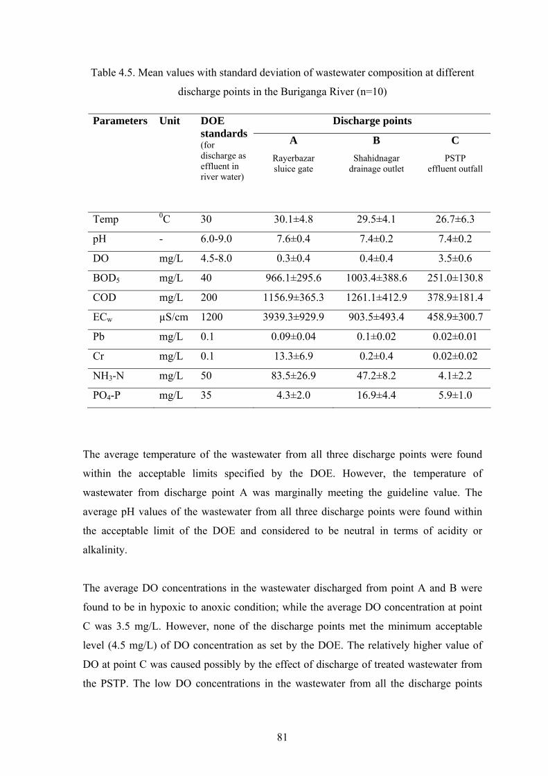
Table 4.5. Mean values with standard deviation of wastewater composition at different

discharge points in the Buriganga River (n=10)

T

w

w

a

th

a

T

fo

C

le

D

th

Discharge points Parameters Unit DOE standards (for discharge as effluent in river water)

A Rayerbazar sluice gate

B Shahidnagar

drainage outlet

C PSTP

effluent outfall

Temp 0C 30 30.1±4.8 29.5±4.1 26.7±6.3

pH - 6.0-9.0 7.6±0.4 7.4±0.2 7.4±0.2

DO mg/L 4.5-8.0 0.3±0.4 0.4±0.4 3.5±0.6

BOD5 mg/L 40 966.1±295.6 1003.4±388.6 251.0±130.8

COD mg/L 200 1156.9±365.3 1261.1±412.9 378.9±181.4

ECw µS/cm 1200 3939.3±929.9 903.5±493.4 458.9±300.7

Pb mg/L 0.1 0.09±0.04 0.1±0.02 0.02±0.01

Cr mg/L 0.1 13.3±6.9 0.2±0.4 0.02±0.02

NH3-N mg/L 50 83.5±26.9 47.2±8.2 4.1±2.2

PO4-P mg/L 35 4.3±2.0 16.9±4.4 5.9±1.0

he average temperature of the wastewater from all three discharge points were found

ithin the acceptable limits specified by the DOE. However, the temperature of

astewater from discharge point A was marginally meeting the guideline value. The

verage pH values of the wastewater from all three discharge points were found within

e acceptable limit of the DOE and considered to be neutral in terms of acidity or

lkalinity.

he average DO concentrations in the wastewater discharged from point A and B were

und to be in hypoxic to anoxic condition; while the average DO concentration at point

was 3.5 mg/L. However, none of the discharge points met the minimum acceptable

vel (4.5 mg/L) of DO concentration as set by the DOE. The relatively higher value of

O at point C was caused possibly by the effect of discharge of treated wastewater from

e PSTP. The low DO concentrations in the wastewater from all the discharge points

81

indicated the possibility of raw sewage released from the adjacent areas which are yet to

be covered by the sewerage network of DWASA.

The average BOD5 concentrations at discharge points A, B and C were found respectively

more than 24, 25 and 6 (six) times higher than the recommended guideline specified by

the DOE. The high values of BOD5 could be linked to increased degradation of organic

content (such as sewage) in the wastewater and thus causing the very low concentration

of DO. Such high concentration of BOD5 would most likely affect the natural assimilating

capacity of the river and a reduction of BOD5 levels are essential in order to protect the

quality of the river water. Moreover, the impact of such high concentration of BOD5 in

the wastewater were reflected in the state of river water quality (Figure 4.9), where during

the dry season the BOD5 levels never reached the DOE guideline along the full length of

the river. Station 2 (receptor point) was worst affected most likely because of the impact

of BOD5 loading from discharge points A and B

The average COD concentrations at discharge points A, B and C were found respectively

more than five, six and two times higher than the recommended guideline of the DOE.

These values were correlated to BOD5 values and indicated the presence of industrial

waste (oxidisable inorganic chemicals) in the effluent. The extent of COD pollution was

so high that the river water could never (including both dry and wet seasons) reach up to

the acceptable level of DOE guideline (Figure 4.11).

The average ECw level of the wastewater discharged from point A was more than three

times higher than the DOE guideline, while the levels were within the guideline values

for discharge points B and C. This was most likely caused by the use of salts while

processing the raw hides within the tanneries (BKH 1995), which were located within the

drainage area of discharge point A. Although the level of ECw in wastewater from

discharge point A and B remained below the acceptable levels, Figure 4.13 indicated that

during the dry season the ECw level in the river water never dropped below the acceptable

level. This was probably because the salts which were being discharged through the

wastewater did not get enough water or time to be diluted within the length of the river.

The Pb concentration in wastewater discharged from points A and B marginally met the

DOE guideline values and thereby probably the concentration levels within the river

82

water were found below the acceptable level. However, appropriate measures should be

taken to identify the sources of this non-decaying toxic substance before its level exceeds

the acceptable limits. The wastewater from discharge point A contained very high Cr

concentration, which was detrimental for the river ecosystem. Compared to discharge

point A, relatively low concentration of Cr was found in the wastewater from discharge

point B, but that value also exceeded the limit of the DOE guideline. The high

concentrations of Cr were most likely a result of the effluent released from the tannery

industries (as mentioned earlier in section 4.3.7) and were eventually being drained off

into the Buriganga River through the discharge points A and B.

The results showed that the discharge point A exceeded the DOE limit of NH3-N

concentration by about two times, while the concentration was found within the limit at

discharge point B and C. The high concentration of NH3-N from discharge point A is

most likely causing a negative impact on river water quality at stations 2 and 3 (Figure

4.19). The PO4-P concentrations at all three discharge points were found within the DOE

acceptable levels.

4.5 Flow rates of wastewater

The flow rates of wastewater from the three discharge points were estimated following

the methodology as described in section 4.2.3. The results are presented in Figure 4.23.

The data on observed average velocities and the calculated flow rates on ten different

occasions for each discharge point are provided in Table G.1 (Appendix G).

0.000

0.500

1.000

1.500

2.000

2.500

1 2 3 4 5 6 7 8 9 10

Observation days

Flow

rate

(m3/

sec)

Discharge point-A Discharge point-B Discharge point-C

Figure 4.23. Flow rates of waste water at different discharge points

83

From these data, the average flow rates for three discharge points were estimated as 0.995

m3/s at Rayerbazar sluice gate, 0.819 m3/s at Shahidnagar drainage outlet and 1.476 m3/s

at PSTP effluent outfall. These results were used to calculate the pollution loading rate of

BOD5 in Buriganga River which is discussed in the following section.

4.6 Loading rates of BOD5 at discharge points

The BOD5 loading rates from the discharge points were estimated as discussed in section

4.2.4 and the results are presented in Table 4.6.

Table 4.6. BOD5 loading rate in the Buriganga River

Discharge points

Average flow rate

(m3/s)

Average BOD5

concentration (mg/L)

BOD5 loading rate

(tons/day)

Total BOD5 loading

(tons/day)

A 0.995 966 83 B 0.819 1003 71 C 1.476 251 32

186

The total loading of BOD5 in the Buriganga River was estimated as 186 tons/day.

Compared to the latest available study (Magumdar 2005), the BOD5 loading in the

present study increased at a rate of 12.5 percent per year, while the rate increased at 13.8

percent per year between 1996 and 2003 (Figure 4.24).

020406080

100120140160180200

Rahman and Rana(1996)

Magumdar (2005)(based on 2003 data)

Present study (2008-09)

Tota

l loa

ding

of B

OD

5 (to

ns/d

ay)

Figure 4.24. Estimated loading rate of BOD5 in the Buriganga River

84

Overall, the results on BOD5 loading rates showed that the contribution of pollution into

the Buriganga River followed the order as Discharge point A>Discharge point B>

Discharge point C. The drainage area and the size of population were found more for

discharge point B compared to discharge point A. However, according to the estimations,

discharge point B was contributing more pollution than discharge point A. This was

possibly because of presence of greater number of industries (which do not have adequate

wastewater treatment facilities) within the drainage area of discharge point A. Discharge

point C contributes the least of pollution possibly because partially treated effluent (from

the PSTP) is discharged through this point.

4.7 Transfer coefficients for discharge-receptor pairs

One of the important bases of the economic model formulation for pollution abatement

policy analysis in this research is the calculation of a set of transfer coefficients that

conveys the water quality response at a receptor point as a result of release of pollutant at

a discharge point (source of pollution). Burn (1989) defined these coefficients as the

function of physical characteristics of the portion of water body that provides the pathway

from the discharge point to the receptor point. Hence, the transfer coefficients are used in

simulating pollutant flows and they represent the degree to which pollution

concentrations at a specific receptor point are increased by a one-unit increase in

emissions from a specific discharge point (Tietenberg 2006). Generally, the transfer

coefficients depend upon the flow, travel time and the geometry of the connecting

pathway, as well as the reaction kinetics for any biological and chemical reactions that

may occur in the water body (Burn 1989).

The nature of the BOD5 is that it is a spatially distributed pollution, so the effluent

discharges may not affect the quality of water (increase/decrease in DO concentration) at

the point of discharge, but can affect the quality downstream (Eckenfelder 1980). Thus

the DO transfer coefficients represent the increase in DO (mg/L) at receptor points

resulting from decrease of BOD5 (per ton/day) at discharge points. The transfer

coefficients of the oxygen demanding wastes were calculated from the Streeter Phelps

model of DO concentration (Streeter and Phelps 1925). They represent the amount of DO

that is required for each ton/day of BOD5 loading at each discharge point along the river.

The inputs to the Streeter Phelps model that were required for each discharge-receptor

85

pair were: the flow, the travel time, the deoxygenation and the reaeration rate coefficient,

and the BOD5 loading rates at the discharge points. The functional relationship for the

transfer coefficient model was of the following form (Burn 1989, p.1015):

( )1 1 2

2 1

i ijij iji

i K Kij

ij ij

L K

Q K Kt td e e− −⎡ ⎤= −⎣ ⎦− (4.3)

where,

ijd = DO transfer coefficient;

jQ = flow at the receptor location;

ijt = travel time from the discharge to the receptor point;

1i

K = deoxygenation rate coefficient;

2ij

K = reaeration rate coefficient; and

iL = BOD5 loading rate at the discharge point

The average values of deoxygenation rate coefficients and reaeration rate coefficients for

different segments of the Buriganga River were adapted from Ahmed and Mohammed

(1988) as shown in Table 4.7. The input data for the Streeter Phelps model for different

discharge-receptor pairs are provided in Table H.1 (Appendix H). The most deteriorating

condition in terms of BOD5 pollution in a river may occur when the river flow rate is

minimum. In this study, the monthly average flow rates for the years 2005, 2006 and

2008 (Table A.1 in Appendix A) were considered and the lowest value from these was

nominated for the Equation 4.3 to calculate the DO transfer coefficients. The calculated

values of DO transfer coefficients are provided in Table 4.8.

86

Table 4.7. Average values of deoxygenation rate coefficient, and reaeration rate coefficient, for different segments of the Buriganga River

1iK

2ijK

River segments (between discharge and receptor points)

A-2 A-3 A-4 A-5 B-4 B-5 C-5

Deoxygenation rate coefficient,

(day1iK -1)

0.262 0.23 0.256 0.136 0.256 0.171 0.136

Reaeration rate coefficient (day

2ijK

-1)

0.332 0.245 0.337 0.65 0.337 0.49 0.65

Adapted from: Ahmed and Mohammed 1988

Table 4.8. Dissolved oxygen transfer coefficients, ijd

Receptor points of measurement 2 3 4 5

Distance from Bosila bridge(km)

Discharge points

2.5 6.0 10.0 17.0 A 0.0119 0.0258 0.0518 0.0202 B - - 0.0320 0.0319 C - - - 0.0195

4.8 Conclusion

The results for this study showed that the Buriganga River is certainly unfit for

maintaining the aquatic ecosystem. More specifically, the test results revealed that the

river water is unacceptable (as per DOE standards) for the parameters such as DO, BOD5,

COD, NH3-N and Cr during both dry and wet seasons and for ECw during only dry

season. Whilst, temperature, pH, PO4-P and Pb were found within the DOE acceptable

limits in both dry and wet seasons.

The results from the river water quality study also showed no significant statistical

difference between sampling stations (receptor points) in terms of parameters such as

87

temperature, pH, DO, BOD5, ECw, Pb and PO4-P, while the results showed a significant

difference for COD, Cr and NH3-N. The study indicated that the river is mostly affected

near Kholamora (receptor point 2) and Muslimbag (receptor point 3) by the incoming

wastewater from the nearby discharge points. Further, the test results showed that the

incoming wastewater is in hypoxic to anoxic condition with very high concentration of

BOD5, COD, ECw, Cr and NH3-N compared to the DOE guideline values. The study also

established information on BOD5 loading rates, which is required for this research to

analyse the effectiveness of alternative management strategies for pollution mitigation in

the Buriganga River.

88

Date post:	20-Mar-2022
Category:	Documents
Upload:	others
View:	2 times
Download:	0 times

CHAPTER 4 ANALYSIS OF WATER QUALITY AND POLLUTION …

Documents