47
Chapter 4 CPU Scheduling
| Date post: | 15-Mar-2016 |
| Category: |
Documents |
| Upload: | melvin-gray |
| View: | 106 times |
| Download: | 1 times |

Chapter 4
CPU Scheduling

Scheduling concepts
Types of scheduling – Long, medium, short
CPU scheduler
Dispatcher
Scheduling criteria
Kinds of scheduling
Scheduling algorithms
Scheduling algorithm evaluation
Contents

Scheduling• Key to multi-programming• Objective of multiprogramming is to maximize
resource utilization • Not possible to achieve without proper scheduling • All resources are scheduled before use• CPU is primary resource and scheduling CPU is
central to OS• Four types of schedulers: Long term, Short term,
Medium term, I/O
CPU, I/O cycle
• Process execution consists of cycle of CPU execution and I/O operation
• Process alternate between these 2 states• Begins with CPU burst, followed by I/O burst,
again CPU burst …. terminates after a CPU burst• I/O bound jobs have short CPU bursts• CPU bound jobs have long CPU bursts• Durations of CPU bursts have been extensively
measured• Many jobs have more shorter CPU bursts

Process Scheduling

Long Term Scheduler
• Also called as job scheduler• Determines which programs are to be submitted for
processing• Controls the degree of multi-programming• Selects processes from pool and loads them into
memory for execution• Selection is between I/O bound and CPU bound jobs• Executes much less frequently• Needs to be invoked when a process leaves the
system

Medium Term Scheduler
• Part of the swapping function • Usually based on the need to manage multi-
programming• The process can be reintroduced into memory and its
execution can be continued where it left off• If no virtual memory, memory management is also an
issue

Short Term Scheduler
• Also called as CPU scheduler• Makes fine grained decisions of which job to execute
next. That is which job actually gets to use the processor
• Selects from among the processes that are ready to execute and allocates the CPU to one of them
• This scheduler is called often and it executes at least once every milliseconds
• Selects a process from the processes in Ready queue • CPU scheduling decisions occur when a process:
1. switches from running to waiting state2. switches from running to ready state (interrupt
occurs)3. switches from waiting to ready state (ex. after
completion of I/O)4. terminates
• Scheduling under 1, 4 is non preemptive• Scheduling under 2 and 3 is preemptive

Preemptive and non-preemptive scheduling
• New job has to be scheduled in cases of 1 and 4 – non preemptive
• In case of 2 and 3 scheduling is optional – preemptive• Scheduling done when status of ready queue changes• Preemptive scheduling is expensive, hard• Requires extra hardware• Processes can share data• Should be careful and cautious -if one preempted by
another and the shared data referred by the new process• At time of processing system calls, kernel may be busy on
behalf of a process• If preempted, chaos is the result – unless such preemptions
are taken care of the OS

Dispatcher
• Dispatcher module gives control of the CPU to the process selected by the short-term scheduler and this involves:– switching context– switching to user mode– jumping to the proper location in the user
program to restart that program• Dispatch latency – the time taken by dispatcher to
stop one process and start another running• Dispatcher should execute fast because it is invoked
during every process switch

Scheduling Criteria
• CPU utilization – To what percentage CPU is utilized • 40% - lightly loaded and 90% - heavily loaded
• Throughput – No. of processes that complete their execution per unit time (Degree of multiprogramming)• For long processes it could be 1 in an hour and for
short processes it could be 10 per sec • Turnaround time –Time interval between the time of
submission and completion (Execution time)• Includes also waiting times for CPU as well as I/O
devices
Scheduling criteria• Waiting time – sum of all the time waiting in Ready queue
Does not take into account wait time for I/O and I/O operation time
• Response time – amount of time it takes from the time of submission of a job until the first response is produced
In time shared systems small turn around time may not be enough
Response time should be small. It is the time taken to start responding. Does not include time to output that response

Optimization Criteria
• Maximize CPU utilization and throughput• Minimize turnaround time, waiting time and response
time• We optimize average times. Occasionally optimize
extreme measures Ex. Minimize maximum response time
• In time shared systems it is better if variance in response time is minimized
• A system that has reasonable and predictable response time is better than system with small average response time and highly variable
Kinds of Scheduling
• Non-preemptive scheduling: A process runs to completion when scheduled
• Preemptive scheduling: A process may be preempted for another process which may be scheduled. A set of processes are processed in an overlapped manner

Non-preemptive and preemptive scheduling methods
• Non-preemptive: • FCFS – First come first served• SJF – shortest job first and SRTF – shortest
remaining time first• Priority scheduling• Preemptive:• SJF• Priority scheduling • Round robin• Multilevel queue• Multilevel feed back queue

First Come First Served (FCFS)• Example: Process Burst Time
P1 24 P2 3 P3 3
• Assume processes arrive at time 0
The Gantt Chart for the schedule is:
• Waiting time for P1 = 0; P2 = 24; P3 = 27• Average waiting time: (0 + 24 + 27)/3 = 17
P1 P2 P3
24 27 300

FCFS Scheduling Suppose processes arrive as: P2 , P3 , P1 .• The Gantt chart for the schedule is:
• Waiting time for P1 = 6; P2 = 0; P3 = 3• Average waiting time: (6 + 0 + 3)/3 = 3• Much better than previous case
P1P3P2
63 300
FCFS scheduling
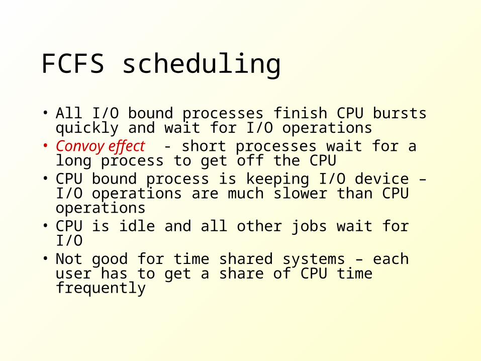
• All I/O bound processes finish CPU bursts quickly and wait for I/O operations
• Convoy effect - short processes wait for a long process to get off the CPU
• CPU bound process is keeping I/O device – I/O operations are much slower than CPU operations
• CPU is idle and all other jobs wait for I/O• Not good for time shared systems – each user has
to get a share of CPU time frequently

Shortest-Job-First (SJF) Scheduling
• In fact it is shortest next CPU burst• Assume CPU burst length for each process in ready
queue are known • Two schemes:
– Non-preemptive – once CPU assigned, process not preempted until its CPU burst completes
– Can be preemptive – if a new process with CPU burst less than remaining time of current, preempt Shortest-Remaining-Time-First (SRTF)
• SJF is optimal – gives minimum average waiting time for a given set of processes

Example of Non-Preemptive SJF
Process Burst TimeP1 16 P2 3 P3 4
SJF (non-preemptive) The Gantt Chart for the schedule is:
Here, the waiting time for P1 is 7ms, P2 is 0ms, P3 is 3ms.• Average waiting time = (7 + 0 + 3 )/3 =10/3=3.33 ms.
P1P3P2
73 230

Example of Preemptive SJF
Process Arrival time Burst TimeP1 0 8 P2 1 4 P3 2 9
P4 3 5SJF (preemptive) The Gantt Chart for the schedule is:
• Average waiting time = (10-1) +(1-1) +(17-2)+(5-3)/4 = 26/4 =6.5ms.
p1 p2 p4 p1 p3
0 1 5 10 17 19
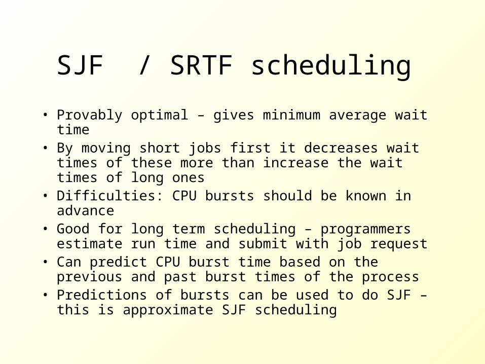
SJF / SRTF scheduling • Provably optimal – gives minimum average wait time • By moving short jobs first it decreases wait times of these
more than increase the wait times of long ones• Difficulties: CPU bursts should be known in advance• Good for long term scheduling – programmers estimate
run time and submit with job request• Can predict CPU burst time based on the previous and past
burst times of the process• Predictions of bursts can be used to do SJF – this is
approximate SJF scheduling
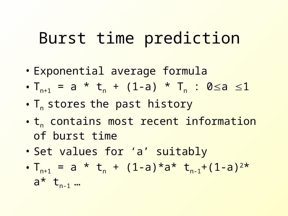
Burst time prediction
• Exponential average formula• Tn+1 = a * tn + (1-a) * Tn : 0a 1
• Tn stores the past history
• tn contains most recent information of burst time
• Set values for ‘a’ suitably• Tn+1 = a * tn + (1-a)*a* tn-1+(1-a)2* a* tn-1 …

Priority Scheduling• Priority number (integer) associated with process• SJF and SRTF are special cases of general priority scheduling • Larger the burst time lower is the priority• CPU allocated to process with highest priority• Can be preemptive or non preemptive• Preemptive priority scheduling will preempt the CPU if a high priority
job arrives to ready queue• Problem: Starvation / indefinite blocking low priority processes
may never execute• Solution: Aging increasing gradually the priority of processes
which are waiting in the system for CPU for a long time• Ex: If priority is 127 (low) decrement by 1 for every 15 minutes of
wait – takes 32 hours to get the priority 0.

Example of priority scheduling Process Burst Time (ms) priority
P1 8 3 P2 2 1 P3 1 3 P4 3 2
p5 4 4
• Average waiting time = wait times of (p1+p2+p3+p4+p5)/5
= (5+0+13+2+14)/5= 34/5 = 6.8 ms
p2 p4 p1 p3 p5
0 1 5 13 14 18

• Designed for time-sharing systems• Jobs get the CPU for a fixed time (quantum time or
time slice)• Similar to FCFS, but with preemption - CPU interrupted at regular intervals• Needs hardware timer• Ready queue treated as a circular buffer • Process may use less than a full time slice• They terminate and scheduling take place• If process is incomplete at the end of time slice, they join end of ready queue• With n processes and quantum = q, each process waits
for at most (n-1)*q
Round robin scheduling
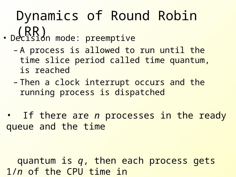
• Decision mode: preemptive – A process is allowed to run until the time slice period
called time quantum, is reached– Then a clock interrupt occurs and the running process
is dispatched
Dynamics of Round Robin (RR)
• If there are n processes in the ready queue and the time quantum is q, then each process gets 1/n of the CPU time in chunks of at most q time units at once. No process waits more than (n-1)q time units.

Performance of RR
• Depends on quantum• Extremes:• Very large – FCFS• Very small (1 ms) – processor sharing • Processes get a feel that each one owns a processor with
speed = 1/n of the single processor• Context switching effect to be considered• Small quantum – Context switches are frequent • CPU will spend lot of time on switching • If context switch time is 10% of quantum, 10% of CPU
time spent on switches
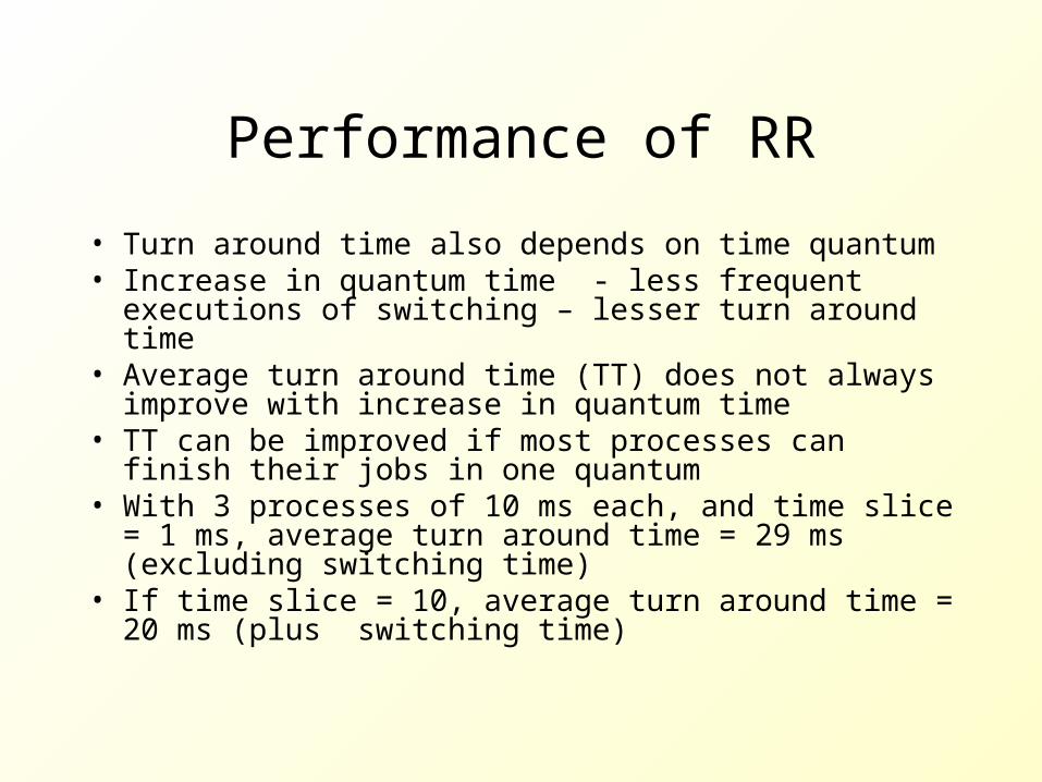
Performance of RR
• Turn around time also depends on time quantum• Increase in quantum time - less frequent executions of
switching – lesser turn around time • Average turn around time (TT) does not always improve
with increase in quantum time• TT can be improved if most processes can finish their jobs
in one quantum• With 3 processes of 10 ms each, and time slice = 1 ms,
average turn around time = 29 ms (excluding switching time)
• If time slice = 10, average turn around time = 20 ms (plus switching time)
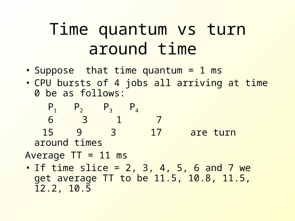
Time quantum vs turn around time
• Suppose that time quantum = 1 ms• CPU bursts of 4 jobs all arriving at time 0 be as
follows: P1 P2 P3 P4
6 3 1 7 15 9 3 17 are turn around timesAverage TT = 11 ms• If time slice = 2, 3, 4, 5, 6 and 7 we get average TT
to be 11.5, 10.8, 11.5, 12.2, 10.5

Round-Robin Example
ProcessArrivalTime
ServiceTime
1
2
3
4
5
0
2
4
6
8
3
6
4
5
2

Example of RR with Time Quantum = 20
Process Burst TimeP1 53
P2 17
P3 68
P4 24
• The Gantt chart is:
P1 P2 P3 P4 P1 P3 P4 P1 P3 P3
0 20 37 57 77 97 117 121 134 154 162

Features of RR
• All processes gets equal share of the CPU• Typically RR gives longer turnaround time than SJF, but better
response time – good for time-sharing• Short time slices gives better response time• Simple, low overhead, works for interactive systems
If quantum too small, too much time wasted in context switching If too large, reduces to FCFS
Typical value: 10 - 100 ms Rule of thumb: Choose quantum so that large majority
(80-90%) of jobs finish CPU burst in one quantum

Multilevel queue scheduling
• This scheduling partitions the ready queue into several separate queues.
Ex: Ready queue can be logically divided into separate queues based on the idea that jobs can be categorized as: - foreground (interactive) - background (batch)
• Assign high priority for type 1 jobs - externally• These two categories have different response time requirements –
make 2 queues • Each queue has its own scheduling algorithm:
foreground – RR background – FCFS
• Method is complex but flexible
•.

Multilevel queue scheduling
• Scheduling must be done among the queues –fixed priority preemptive• All foreground jobs are served and then background attended to only when foreground queue empty• Another method -using time slice between the queues: • Each queue gets a certain amount of CPU time which it can schedule amongst its processes i.e., 80% to foreground in RR; 20% to background in FCFS

Multilevel Queue Scheduling
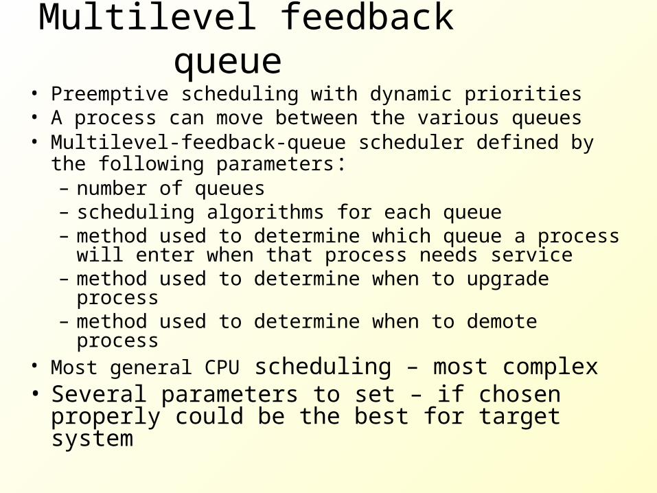
Multilevel feedback queue • Preemptive scheduling with dynamic priorities• A process can move between the various queues• Multilevel-feedback-queue scheduler defined by the following
parameters:– number of queues– scheduling algorithms for each queue– method used to determine which queue a process will enter
when that process needs service– method used to determine when to upgrade process– method used to determine when to demote process
• Most general CPU scheduling – most complex• Several parameters to set – if chosen properly could be
the best for target system

Multilevel Feedback Queues

Example of Multilevel Feedback Queue• Three queues:
– Q0 : time quantum 8 milliseconds– Q1 : time quantum 16 milliseconds– Q2 : FCFS
• Scheduling :– A new job enters queue Q0 which is served FCFS. When
it gets CPU, job receives 8 milliseconds. If it does not finish in 8 milliseconds, job is moved to queue Q1.
– At Q1 job is again served FCFS and receives 16 additional milliseconds. If it still does not complete, it is preempted and moved to queue Q2.
– Could be also vice versa.

Example of Multilevel Feedback Queue

Comparison of algorithms
• Which one is best ?• The answer depends on:
– on the system workload (extremely variable)– hardware support for the dispatcher– relative weighting of performance criteria
(response time, CPU utilization, throughput...)– The evaluation method used (each has its
limitations...)• Hence the answer depends on too many factors to give
any...

Scheduling Algorithm Evaluation
• Deterministic modeling • Queuing models• Simulation• Implementation

Algorithm Evaluation
• Analytic evaluation: - Deterministic modeling : takes a particular predetermined
workload and compares the performance of each algorithm for that workload. Simple and easy to do; but requires exact numbers for input which is hard to get for any given system. Not realistic.
• Queuing models (stochastic model ) : - Knowing the job arrival rates and service rates we can compute CPU utilization, average queue length, average waiting time, etc.
- This is a separate area called queuing-network analysis.

• Experimental method: - Simulation :
- Involves programming a model of the system - Results are of limited accuracy
• Implementation: - Implement the algorithm and study the performance - It is the best way to study and compare the performance of different algorithms - It is expensive and time consuming

Evaluation of CPU Schedulers by Simulation Evaluation of CPU Schedulers by Simulation

Evaluation by implementation• Best way to tune parameters of OS is to implement and let it be
in use and collect statistics• Change parameters if needed• Difficulties:• Changing environment – Jobs may not be of same type and
number always• Clever users can change style of code • Non-interactive programs can be changed as interactive (dummy
inputs) so that his job gets high priority • Big jobs may be broken down to several small ones • Flexible OS will allow system managers change settings and
priorities• If pay checks are needed urgently, this job’s priority can be
changed temporarily and set back to low after the job is done• Such systems are rarely available


