52 CHAPTER 4 DEVELOPMENT OF A USER DEFINED FRACTAL ANTENNA In this chapter a newly shaped fractal geometry using PSO and BFO with curve fitting is presented. The aim of using these biologically inspired optimization techniques is to find the geometrical descriptors of the antenna for the required user defined frequency. In order to assess the effectiveness of the presented method, a set of representative simulations had done and the results were compared with the measurements from experimental prototypes fabricated as per the design specifications obtained from the optimization procedure. The antenna characteristics have been studied using extensive numerical simulations and were experimentally verified. 4.1 Introduction The inspired combination of fractal geometry with the electromagnetic theory has led to the development of a new class of antennas, the fractal antennas [89]. In the quest for compact and multiband antennas, fractals have played a major role and several fractal antennas have been studied extensively in recent studies [102]. Fractal antennas are extensively utilized in wireless communication systems by exploiting their low-profile features [49], [78]. Fractal antennas use the self-similarity property of fractal geometries to resonate the antenna at a number of frequency bands [21], [24]. Whereas, in order to be a useful radiator, it is necessary for the fractal antennas to resonate at user-defined frequencies. However, some techniques have been
Transcript
52
CHAPTER 4
DEVELOPMENT OF A USER DEFINED
FRACTAL ANTENNA
In this chapter a newly shaped fractal geometry using PSO and BFO with
curve fitting is presented. The aim of using these biologically inspired optimization
techniques is to find the geometrical descriptors of the antenna for the required user
defined frequency. In order to assess the effectiveness of the presented method, a set
of representative simulations had done and the results were compared with the
measurements from experimental prototypes fabricated as per the design
specifications obtained from the optimization procedure. The antenna characteristics
have been studied using extensive numerical simulations and were experimentally
verified.
4.1 Introduction
The inspired combination of fractal geometry with the electromagnetic theory
has led to the development of a new class of antennas, the fractal antennas [89]. In
the quest for compact and multiband antennas, fractals have played a major role and
several fractal antennas have been studied extensively in recent studies [102]. Fractal
antennas are extensively utilized in wireless communication systems by exploiting
their low-profile features [49], [78]. Fractal antennas use the self-similarity property
of fractal geometries to resonate the antenna at a number of frequency bands [21],
[24]. Whereas, in order to be a useful radiator, it is necessary for the fractal antennas
to resonate at user-defined frequencies. However, some techniques have been
53
proposed to shift the resonant frequencies of the fractal shaped antennas, but it is a
challenging task to design the fractal antenna shape according to user-defined
frequencies. The challenge is to determine the geometric parameters of the antenna,
such as the antenna dimensions and the feed position, to achieve the best design that
satisfies a certain criterion. In recent years, many efforts have been expanded on the
parametric study of various fractal antennas. As a result, irregular structures are
gaining popularity due to their ability to achieve large bandwidth or multi-band
operation [35], [63], [118]. But, these studies are not systematic and the conclusions
are highly dependent on the antenna under investigation. Consequently, a trial-and-
error process is inevitable in most fractal antenna designs [116], [169]. Over the years,
biologically inspired computational techniques have gained popularity among
scientists in every branch of engineering. Scientists have tried various techniques such
as the artificial neural network, Particle-Swarm Optimization, the genetic algorithm
(GA), bacteria-foraging optimization (BFO), and many others for finding an easy
solution to their problem. The robustness of these techniques has been tested in
problems encompassing every engineering field. For the last decade or so, microwave
engineers have frequently used these techniques [128]. However, available studies
have shown lengthy optimization procedures for such type of designs. It is interesting
to find that evolutionary algorithms (EAs), such as PSO and BFO are also used in
planar antenna design. The PSO‟s simplicity, ease of implementation, and flexibility
make it extremely appealing for multi-dimensional electromagnetic designs [105].
BFO has drawn the attention of researchers and engineers because of its efficiency in
solving real-world optimization problems arising in several application areas. The
PSO and BFO are used in conjunction with the numerical electromagnetic solver and
are found to be a revolutionary approach to antenna design and optimization. This
54
procedure was adopted to bypass the repeated use of the simulator for analysis of the
fractal structure. It needs hundreds of simulations in order to find an optimized
structure of the antenna to resonate at user-defined frequencies [65], [66].
This work demonstrates design and fabrication of new fractal antenna using PSO and
BFO algorithms, for wireless communication and their application in health care.
Telemedicine facilitates the provision of medical aid from a distance. Decision
makers in the healthcare industry are shifting to mobile and wireless technology, to
improve the quality of their patient care in critical applications [107]. Correct and
timely transmission of medical data and information is necessary for the safety and
effectiveness of both wired and wireless medical systems [37], [147]. In recent years,
various Electromagnetic simulation software are available for designing of fractal
antennas, amongst, the one of the powerful electromagnetic simulation software is
IE3D. In this work full wave IE3D simulator was used to predict the performance of
antenna.
4.2 Design Implementation
New fractal geometry for patch antenna is presented in this work. Figure 4.1
shows the zero, first and second iteration of the proposed antenna structure. Fractal
antenna of different iteration orders can be designed by dropping same structured
elements on the patch, whose scale factor is 1/3 without changing the physical
parameters of the antenna. In this presented work only the first and the second
iterations are considered since high order iterations do not make significant effect on
antenna properties. The antenna is designed on FR4 substrate with dielectric constant,
Єr = 4.4. A 50Ω CPW fed transmission line which consists of a single strip is used to
feed the antenna. Two finite ground planes with the same size are placed
symmetrically at both sides of CPW line. The patch size is characterized by the length
55
L, width W and thickness, h. The dimensional parameters of the proposed antenna are
detailed in Table. 4.1. There is a technique to produce the fractals called initiator-
generator construction. This technique begins with a specified initiator, and a
generator which is applied repeatedly in a lower scale to form the fractal geometries
[23], [24].
Table 4.1 Dimensional Parameters of Proposed Antenna
Parameters Values
Dielectric constant, Єr 4.4
Width of the antenna, W 24 mm
Width of feed strip 3 mm
Gap between strip and ground plane 1.5 mm
Space between patch and ground plane, g 1.8 mm
Length of ground plane, Lp 21.6 mm
Width of ground plane, Wp 31.5 mm
(a) (b)
(c)
Figure 4.1 Geometry of the proposed fractal antenna (a) zero iteration (b) first
iteration (c) second iteration
56
4.2.1 IFS Algorithm for Fractal Geometry
An iterative function system (IFS) can be effectively used to generate the
standard fractal geometry. A set of affine transformations forms the IFS for its
generation [21, 22]. The transformations for different iterations can be achieved using
Equation 4.1.
f
e
y
x
dc
ba
Y
Xw (4.1)
where a, b, c, d, e and f are real numbers, such that a, b, c and d control rotation and
scaling, while e and f control linear translation. The transformations to obtain the
segments of the generator are:
y
x
y
xw
3
10
03
1
'
'1 (4.2)
3
20
3
10
03
1
'
'2
y
x
y
xw (4.3)
3
23
2
3
10
03
1
'
'3
y
x
y
xw (4.4)
03
2
3
10
03
1
'
'4
y
x
y
xw (4.5)
where w1, w2, w3 and w4 are set of affine linear transformations, and let M be the
initial geometry then the generator is obtained as:
57
M1 = w1 (M) U w2 (M) U w3 (M) U w4 (M) (4.6)
This procedure can be repeated for all higher iterations of the structure. Scale factors
in these transformations are such that they lead to a self-similar structure, a fact that is
visually apparent from Figure 4.1. The similarity dimension can be interpreted as a
measure of the space filling properties and complexity of the fractal shape. The fractal
similarity dimension is given by the Equation 4.7, where „n‟ is the total number of
distinct copies and „r‟ is the scale factor of the consecutive iteration. The similarity
dimension of the geometry can, thus, be calculated as [158]:
D = = = 1.261 (4.7)
4.2.2 Curve Fitting Implementation
The MATLAB software has been used for curve fitting method to form a
relationship between the design parameters (h, L) and the corresponding resonant
frequency (f) of the proposed fractal geometry. In case of fractal geometries their
resonant properties depend on the dimensions of the structure. EM simulator has been
used to generate data sets by varying the height and length of the antenna and after
applying these values, following equation was obtained that represents the mapping of
resonant frequency with these design parameters:
f = (0.063 h2 - 0.001318 L
2 - 0.8472 h + 0.03632 L + 7.212) (4.8)
4.2.3 PSO Implementation
The basic concept of PSO lies in accelerating each particle toward its pbest
and the gbest locations, with a randomly weighted acceleration at each time step as
shown in Figure 4.2 [66, 71]. The role of the PSO was to find the optimized values of
the length and height which defines the best fractal structure for the specific
frequency of operation. These two parameters were defined with suitable lower and
58
upper bounds that gives two-dimensional solution spaces for which PSO searched for
the optimal parameters of the proposed fractal structure. Then a fitness function was
developed that gives a single number after taking the values of these parameters [64-
66]. The following fitness function was formed to find the structure of the fractal
geometry to work at the user defined frequency.
Fitness function = (5.8 – f) 2
(4.9)
The instantaneous frequency f, was developed using curve fitting method.
Figure 4.2 Basic concept of PSO
The particles position can be modified according to the following equations [128]:
SN+1
= SN
+V N+1
, (4.10)
VN+1
= w V N
+ c1r1 (Pbest - SN) + c2r2 (gbest - S
N) (4.11)
where VN is the particle velocity; S
N is the particle displacement, Pbest is particle best
position; gbest is global best position, w is inertial weight. On completion of the
iterative process, by terminating the optimizer iteration when it reaches the global
margin of 2×10⁻⁴
, the PSO produces the optimized values of the two parameters h and
59
L. For the present problem, the input parameters taken for PSO are detailed in Table
4.2 and the pseudo code for the PSO is presented Figure 4.3
Table 4.2 Input parameters of PSO.
S.no. Parameters Values
1 Population size 10
2 Inertial weight, w 0.6
3 Acceleration terms, c1and c2 2
4 Random numbers, r1, r2 0.9
5 Number of iterations 100
For each particle
Initialize particle
Do until maximum iterations or minimum error criteria
For each particle
Calculate Data fitness value
If the fitness value is better than pBest
Set pBest = current fitness value
If pBest is better than gBest
Set gBest = pBest
For each particle
Calculate particle Velocity
Use gBest and Velocity to update particle Data
Figure 4.3 Pseudo code for the PSO [128]
60
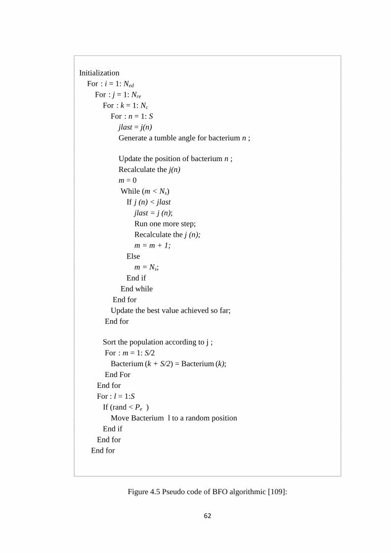
4.2.4 BFO Implementation
In the BFO optimization technique variable need to optimize can take as the
location of bacterial in the search. The main purpose of the BFO in this case is to find
the optimized values of the length of the antenna (L) and height of substrate (h) that
defines the best fractal geometry to make it resonate on required frequency. The goal
of parameter estimation is to find the best values for a set of model parameters. In
order to start the BFO process these parameter (h, L) was initialized with suitable
lower and upper bound that defines a solution space in which the BFO searches for
the optimal design parameter of the geometry. The input variables of BFO for the
proposed antenna are detailed in Table 4.3 and pseudo code of BFO algorithm [109]
is given in Figure 4.5. The fitness function for the present problem is given by
Equation 4.12.
Fitness function = (5.8 – f) 2
(4.12)
Where f is the processed output from cost function, corresponding to the required
frequency of the antenna.
Table 4.3 Input parameters of BFO
Parameters Details of Parameters Values of
Parameters
S Total number of bacteria in the population 10
Nc Number of chemotactic step 25
Ns Swimming length 4
Nre Number of reproduction steps 4
Ned Number of elimination-dispersal events 2
Ped Elimination-dispersal probability 0.25
4.2.5 Design Steps of Proposed Antenna
The step-by-step design procedure may be summarized as follows:
Step1. Input the desired frequency.
61
Step2. Optimization loop, with the use of curve fitting relation, determines the
design dimensions of the new fractal antenna.
Step3. If the antenna resonates on the desired frequency the design process is
terminated.
Step4. Use the optimized dimensions to fabricate the antenna for experimental
validations.
Figure 4.4 shows the flow graph of the entire design process of new fractal
antenna design.
Figure 4.4 Methodology used for new fractal antenna design
62
Initialization
For : i = 1: Ned
For : j = 1: Nre
For : k = 1: Nc
For : n = 1: S
jlast = j(n)
Generate a tumble angle for bacterium n ;
Update the position of bacterium n ;
Recalculate the j(n)
m = 0
While (m < Ns)
If j (n) < jlast
jlast = j (n);
Run one more step;
Recalculate the j (n);
m = m + 1;
Else
m = Ns;
End if
End while
End for
Update the best value achieved so far;
End for
Sort the population according to j ;
For : m = 1: S/2
Bacterium (k + S/2) = Bacterium (k);
End For
End for
For : l = 1:S
If (rand < Pe )
Move Bacterium l to a random position
End if
End for
End for
Figure 4.5 Pseudo code of BFO algorithmic [109]:
63
4.3 Results and Discussion
4.3.1 Resonant Parameters of Proposed Fractal Structure
In order to access the effectiveness of the proposed design, developed
methodology were used to draw the structure of antenna. The simulation tool adopted
for evaluating the performance of the fractal antenna is IE3D software, which exploits
the method of moments to solve the electric field integral equations. Figure 4.6 shows
the S11-parameter for all the three iterations of proposed fractal antenna that is zero,
first and second iteration. S-parameters describe the input and output relationship
between ports or terminals in an electrical system. The most commonly used
parameter with regards to antennas is S11. It indicates how much power is reflected
from the antenna. If the value of S11 is equal to zero dB, then all the power is reflected
from the antenna and nothing is radiated. If the value S11 is equal to -10 dB, this
means that if 3 dB of power is delivered to the antenna and -7 dB is the reflected
power. The remainder of the power was delivered to the antenna. This accepted power
is either radiated or absorbed as losses within the antenna system. Generally antennas
are designed to be low loss and ideally the majority of the power delivered to the
antenna is radiated [16].
As expected, it was illustrated that with increase in the iterations, resonant
frequency decreases and this satisfy the self-similarity property of fractal geometries.
The simulated resonant characteristics of the proposed antenna are reported in Table
4.4. It can be noticed that there is an increase in the impedance bandwidth of the
proposed structure when the iterations of the fractal antenna increases, with
substantial improvement in the impedance matching of the antenna.
64
Figure 4.6 Simulated S11 parameter of proposed antenna for zero, first and second
iteration.
Table 4.4 Resonant performance characteristics of proposed antenna
No. of
Iteratio
ns
Resona
nt
Frequen
cy
(GHz)
Reflection
Coefficient
(dB)
Bandwidth
(%)
Input
Impedance
(ohms)
Antenn
a
Efficien
cy (%)
Radiati
on
Efficie
ncy
(%)
Zero 6.09 -25.21 13.73 44.80 54.47 55.33
First 6.03 -18.95 15.91 52.84 61.42 61.44
Second 5.727 -35.87 22.41 51.54 85.02 85.08
4.3.1.1 Input Impedance
As EM waves travel through the different parts of the antenna system, from
the source to the feed line to the antenna and finally to the free space, they may
encounter differences in impedance at each interface. The input impedance is the ratio
between voltage and currents at antenna ports [16]. The impedance of the antenna has
been adjusted through the design process to be matched with the feed line and have
less reflection to the source. A typical input characteristics Zin = Rein + jImin of the
first three iterations for the proposed fractal antenna are shown in Figure 4.7 and
Figure 4.8, where Zin is the input impedance , Rein is the real part of the impedance
65
(resistance) and Imin is the imaginary part of the impedance (reactance) . And it is
illustrated that with increase in iterations, the input impedance is improving
significantly, which means that the input impedance of the proposed antenna is
getting better corresponding to the resonating frequency with every next iteration,.
Figure 4.7 Simulated real input impedance of proposed antenna for zero, first and
second iteration.
Figure 4.8 Simulated imaginary input impedance of proposed antenna for zero, first
and second iteration.
66
4.3.1.2 Voltage Standing Wave Ratio (VSWR)
The voltage standing wave ratio is also known as standing wave ratio and it is
a function of the reflection coefficient, which describes the power reflected from the
antenna [16]. The VSWR of the proposed antenna for zero, first and second iteration
is shown in Figure 4.9. The presented results shows that the value of VSWR for the
resonating frequency band of all the three iterations is less than 2, which is the
requirement of an efficient antenna and reveals that the antenna is well matched.
Figure 4.9 Simulated VSWR of proposed antenna for zero, first and second iteration.
4.3.1.3 Antenna Efficiency and Radiation Efficiency
The antenna efficiency is associated with the power delivered to the antenna
and the power radiated or dissipated within the antenna system [11]. The antenna
efficiency and radiation efficiency of the proposed antenna is shown in Figure 4.10
for all the three iterations and it is found that with increase in iteration, the antenna
and radiation efficiency increases for the respective resonating frequency.
67
(a)
(b)
(c)
Figure 4.10 Antenna and Radiation efficiency of proposed antenna for (a) zero
iteration (b) first iteration and (c) second iteration
68
4.3.1.4 Smith chart
The smith chart is a graphical method of displaying the impedance of an
antenna, which can be a single point or range of points to display the impedance as a
function of frequency. The smith chart of the proposed antenna for all the three
iterations is shown in Figure 4.11. It may be illustrated that impedance of the
proposed antenna is getting better with increase in iterations of the proposed antenna.
(a) (b)
(c)
Figure 4.11 Smith chart of the proposed antenna for (a) zero iteration (b) first iteration
and (c) second iteration
69
4.3.2 Results of Optimization
The design of the proposed antenna has been formulated in terms of an
optimization problem by defining and imposing suitable constraints on resonant
frequency. To obtain a database from simulator for obtaining fitness function, the
height of the substrate (h) and length of the antenna (L) has been varied. The
relationship between these designs parameters and the required frequency was
generated by Curve-fitting method. In order to illustrate the impact and to increase the
confidence in optimization techniques, the proposed antenna was synthesized with
PSO and BFO. The motive behind using these optimization techniques are their
inherent simplicity and cooperative knowledge, compared to the competitive mode in
the other algorithms. The BFO and PSO are quite similar in approach with subtle
differences. Though PSO is a good optimization algorithm, it can be trapped in local
minima and may converge prematurely. However, BFO algorithm attempts to make a
judicious use of exploration and exploitation abilities of the search space and
therefore likely to avoid false and premature convergence in most of the cases. The
graphical comparison for average best solution by varying number of iterations, using
both the techniques is shown in Figure 4.12 and obtained results reveals that BFO
outperforms PSO for most of the iterations. The advantage of BFO is that it is
generalized in nature and for any small patch antenna and higher dielectric constant
(εr < 10), the resonance frequency can be calculated accurately [133]. It concludes
that the BFO algorithm has an edge over PSO in terms of final accuracy and
robustness. To make the comparison fair, population for both the competitor
algorithms were initialized using the same random seed. The second iteration of
proposed antenna has been optimized to resonate at user defined frequency of 5.8
GHz. Figure 4.13 gives the graphical comparison of s-parameters between BFO and
70
PSO. Based on these studies it is observed that the BFO not only provides more
accurate results in terms of required resonating frequency but also outperform in
antenna performance characteristics such as reflection coefficient, radiation efficiency
and bandwidth, than PSO, which is a primary motive for optimization of the proposed
geometry. However, the computational time for PSO is less than BFO. The various
antenna parameters and their simulated results using both the optimization techniques
have been detailed in Table 4.5. It is interesting to note from Table 4.5, that for most
of the cases the BFO algorithm beats its nearest competitor PSO in a statistically
meaningful way.
Figure 4.12 Average best solutions found using PSO and BFO
Table 4.5 Comparison of PSO and BFO results for proposed PHFT antenna.
Paramet
ers
Lengt
h, L
(mm)
Heigh
t, h
(mm)
Reson
ant
Freque
ncy
(GHz)
Reflecti
on
Coeffici
ent (dB)
Bandwidt
h (%)
Radiatio
n
Efficienc
y (%)
Compu
tational
Time
(sec.)
PSO
Results
32.3 1.8 5.70 -35.01 22.50 79.10 1.08
BFO
Results
31.8 1.6 5.78 -36.86 24.34 82.90 8.80
71
Figure 4.13 S11 parameter comparisons of PSO and BFO
4.3.3 Experimental Results
As the BFO provides better required results than PSO so antenna dimensional
parameters obtained using it, is considered further for fabrication process. The
optimized antenna is fabricated using the FR4 substrate having the dielectric constant
of 4.4 and measured to test the accuracy of the proposed structure. The optimized
length and height of the designed antenna are, L = 31.8 mm and h = 1.6 mm
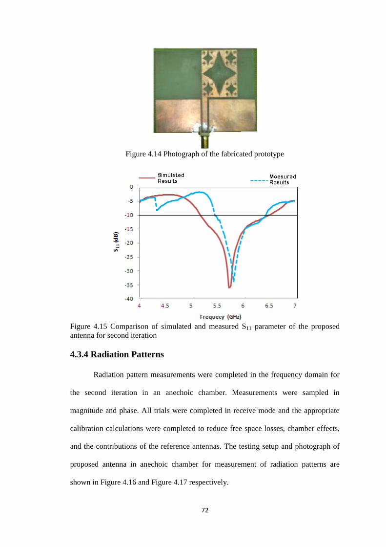
respectively. The photograph of the fabricated antenna prototype is shown in Figure
4.14. The experimental S11 plot obtained using HP 8720B (130 MHz – 20 GHz)
network analyzer, is overlapped with the simulated plot for comparison purpose. The
measured results are in good agreement with the simulated results as shown in Figure
4.15, despite a slight frequency shift of 1.3% from the simulated results. This
frequency shift is mainly because of the fabrication imperfections. The proposed
fractal antenna resonates at 5.8 GHz of ISM (Industrial Scientific and Medical band,
5.725 – 5.875 GHz) which is suitable for wireless Telemedicine applications.
72
Figure 4.14 Photograph of the fabricated prototype
Figure 4.15 Comparison of simulated and measured S11 parameter of the proposed
antenna for second iteration
4.3.4 Radiation Patterns
Radiation pattern measurements were completed in the frequency domain for
the second iteration in an anechoic chamber. Measurements were sampled in
magnitude and phase. All trials were completed in receive mode and the appropriate
calibration calculations were completed to reduce free space losses, chamber effects,
and the contributions of the reference antennas. The testing setup and photograph of
proposed antenna in anechoic chamber for measurement of radiation patterns are
shown in Figure 4.16 and Figure 4.17 respectively.
73
Figure 4.16 Testing setup for measuring radiation patterns
Figure 4.17 Photograph of the proposed antenna in anechoic chamber for the
measurements of radiation patterns
The radiation characteristics of simulated and fabricated antenna were checked
in order to verify the fractal behavior. Figure 4.18 to Figure 4.20 gives the simulated
radiation patterns for all the three iterations and Figure 4.21 showed the measured
radiation patterns for second iteration. It is observed that the proposed antenna
74
exhibits omnidirectional radiation patterns at the y-z plane (H-plane) and “8-shape”
radiation patterns at the x-z plane (E-plane), similar to those of an ideal dipole
antenna. It is illustrated that simulated and measured radiation characteristics are in
good agreement and the proposed antenna is linearly co-polarized antenna.
(a) (b)
Figure 4.18 Simulated radiation patterns for zero iteration at 6.09 GHz (a) H-plane (b)
E-plane
(a) (b)
Figure 4.19 Simulated radiation patterns for first iteration at 6.03 GHz (a) H-plane (b)
E-plane
75
(a) (b)
Figure 4.20 Simulated radiation patterns for second iteration at 5.727 GHz (a) H-plane
(b) E-plane
(a) (b)
Figure 4.21 Measured radiation patterns for second iteration at 5.80 GHz (a) H-plane
(b) E-plane
4.3.5 Gain v/s Frequency Plot
The ability of an antenna to direct the radiated power in a given direction is
specified in terms of its gain. The Gain v/s Frequency is one of the ways to assess the
antenna performance. The measured and simulated gain of the proposed antenna is in
good agreement as shown in Figure 4.22. The achievable measured gain at the desired
resonant frequency (5.8 GHz) is 4.6 dBi.
76
Figure 4.22 Simulated and measured Gain of the proposed fractal antenna.
4.4 Conclusion
In this chapter, a fast, flexible and accurate procedure for making fractal
antenna is proposed, which is easy to use from the designer's point of view. The
antenna geometry is based on a new planar fractal antenna, whose geometrical
descriptors are determined by means of PSO and BFO. The goal of this work was to
give a conceptual overview of these optimization techniques into the electromagnetic
community. In the presented work, PSO and BFO programs was developed using
equation obtained by curve fitting technique. The BFO out performs in terms of
accuracy and antenna performance than PSO, whereas PSO converges faster than
BFO. An antenna prototype has been successfully implemented in order to assess the
effectiveness and the reliability of the proposed designed geometry. Numerical and
experimental analyses have been carried out, and some representative results are
reported to give an overview of the prototype performance. The measured electrical
parameters confirm the reliability of the antenna and make it feasible for wireless