Chapter 4: Markov Chains

Markov chains and processes are fundamental modeling tools in applications. The reason fortheir use is that they natural ways of introducing dependence in a stochastic process and thusmore general. Moreover the analysis of these processes is often very tractable. But perhaps anoverwhelming importance of such processes is that they can quite accurately model a wide varietyof physical phenomena. They play an essential role in modeling telecommunication systems, servicesystems, and even signal processing applications. In this chapter we will focus on the discrete-time,discrete-valued case, that leads to the appellation Markov chains.

1 Introduction and preliminaries

We restrict ourselves to the discrete-time case. Markov chains (M.C) can be seen first attempt toimpose a structure of dependence in a sequence of random variables that is rich enough to modelmany observed phenomena and yet leads to a tractable structure from which we can perform cal-culations. Supose we had a sequence of r.v.’s Xi and we know say X5, if the X ′is are independentthen this information would say nothing about a future value , say X10, other than the a prioriassumptions that we have on their distribution. O the other hand if they were dependent, unlesswe precisely specify how the probability distributions at one time depend on the distributions atother times there is very little we could do because we know to specify a stochastic process we needto specify the joint distributions. Markov chains (or Markov processes in general) are stochasticprocesses whose future evolution depends only on its current value and not how it reached there.We formalize this idea below.

Definition 1.1. Let Xn be a discrete-line stochastic process which takes its values in a space E.Let A ⊂ E. If

PXn+1 ∈ A|Xo, X1, . . . Xn = PXn+1 ∈ A | Xn

then Xn is said to be a discrete-time Markov process.More generally

PXn+1 ∈ A |FXn = PXn+1 ∈ A |Xn

where FXn = σXu, u ≤ n the sigma-field of all events generated by the process Xk up to n.

WhenE = 0, 1, . . . ,

i.e., a countable set then Xn is said to be a Markov chain.

From now on we will always assume E to be a finite or countable (discrete) set. E is said to bethe state-space of the Markov chain.

From the definition of a Markov chain it is easy to see that if

A ⊂ X0 . . . Xn−1 , B ⊂ Xn+1 , . . .

thenP(A ∩B|Xn) = P(A|Xn) P (B|Xn)

1

Let denote Fn = σXk, k ≤ n and Fn = σXk,K > n Then more generally if A ∈ Fm, B ∈ Fpand m < n < p then:

P(A⋂B|σ(xn)) = P(A|σ(Xn))P(B|σ(Xn))

In other words, for any m ≤ n− 1, p ≥ n+ 1

PXm = i,Xp = j|Xn = k = PXm = i|Xn = k PXp = j|Xn = k

i.e., if Xn is a Markov chain then the future (represented by the process at times > n) and thepast (represented by the process at times < n) are conditionally independent given the process attime n given by Xn. Conditional independence is actually a better way of defining the Markovproperty since it extends readily to the case when the index set is not necessarily the set of integersbut of higher dimension.

From Chapter 1., we know that if we define events An = Xn ≤ an, then if An’s are Marko-vian then the P(An) is determined from the knowledge of P(A0) and the conditional probabilitiesP(Ak+1|Ak). Thus if Xn is Markov, what we really mean is that the events generated by Xnhave the Markovian property, which is equivalent to the distribution at any time is completelydetermined by its initial distribution π(0)(i) = PX0 = i and the conditional distributionsPXk+1 = j|Xk = i for k = 1, 2, . . . n− 1.

The conditional probability

PXk+1 = j|Xk = i = Pij(k)

is called the transition probability of the Markov chain.

If Pij(k) does not depend on the time k then we say that the Markov chain is time-homogeneousor simply homogeneous.

For examplePxk+1, = j/xk = i = Pij

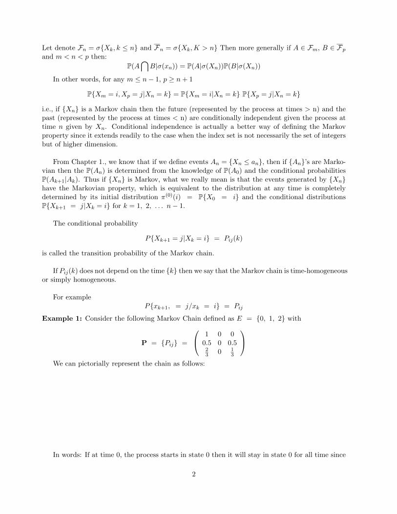
Example 1: Consider the following Markov Chain defined as E = 0, 1, 2 with

P = Pij =

1 0 00.5 0 0.523 0 1

3

We can pictorially represent the chain as follows:

In words: If at time 0, the process starts in state 0 then it will stay in state 0 for all time since

2

the transition probability P0j = 0 if j 6= 0.

If the process starts in state 1 then with probability 1/2 it will be in either (0) or (2) at the nextinstant. In other words, if we observe the chain for a long time the state 1 will only be observed ifthe chain starts there, and over the long run it will be in state 0. Since once it goes to 0 it stays there.

In the sequel we will see that the states 0, 1 and 2 have some special properties. We willfocus our attention on studying the long-run behavior of Markov chains. In fact, it will be seenthat the entire structure is governed by P the matrix of the transition probabilities.

In the following we will use the following notation.

We will denote a Markov chain by (E,P ) where E denotes the state spaceand P the transition probability matrix.

Let us now introduce some rotation which will be used throughout our study of Markov chains.

Pij = PXk+1 = j|Xk = i

P(k)ij = PXk = j|X0 = i, i.e., the conditional probability that the chain is in state j after

k-transitions given that it starts in state i.

π(k)j = PXk = j

andP = Piji, j ∈ E

We now state the first fundamental result which is obeyed by the conditional probabilities of aMarkov chain. The equation is called the Chapman Kolmogorov equation. We saw (in Chapter 2)that any Markov chain must obey this equation.

Theorem 1.1. (Chapman-Kolmogorov Equations)

P(k+l)ij =

∑α ∈ E

P(k)iα P

(l)αj

Proof

PXk+l = j/X0 = i =∑α

PXk+1 = j, Xk = α|X0 = i

(Conditional Probabilities) =∑α∈E

PXk+1 = j|Xk = α, X0 = iPXk = α|X0 = i

(Markov Property) =∑α∈E

PXk+1 = j|Xk = αPXk = α|X0 = i

=∑α∈E

P(k)iα P

(l)αj

3

In the above proof we used the fact that the chain is homogeneous. Another way of stating thisresult is in matrix notation.

Note that by definitionPnij = (Pn)ij

HencePk+l = PkPl .

There are two sub-cases of the Chapman-Kolmogorov equation that are important.

P(k+1)ij =

∑α∈E PiαP

(k)αj : Backward equation

P(k+1)ij =

∑α∈E P

(k)iα Pαj : Forward equation

What they state is that to reach the state j after (k+ 1) steps, the chain starts in state i and goesto state α after the first transition and then goes to j from state α after another k transitions orvice versa.

In a similar vein,

π(k+1)j =

∑α∈E παP

(k)αj

π(k+i)j =

∑α π

(k)α P

(i)αj

Note that by definition of the transition probabilities∑j∈E

P(n)ij = 1 for all n.

Example 2: Consider a homogeneous M.C. (E P )

P =

[P00 P01

P10 P11

]Then it is easy to calculate the powers of P as

P2 =

P 200 + P01P10 P01(P00 + P11)

P10(P00 + P11) P 211 + P01P10

and by induction

Pn =

(1

2− P00 − P11

)(1− P11 1− P00

1− P11 1− P00

)

+(P00 + P11 − 1)n

2− P00 − P11

(1− P00 −(1− P00)−(1− P11) 1− P11

)under the hypothesis |1− P00 − P11| < 1.

4

Hence if P00 , P11 6= 1 then the hypothesis is always satisfied and

limn→∞

Pn =1

2− P00 − P11

1− P11 1− P00

1− P11 1− P00

which means

limn→∞

PXn = 1|X0 = 0 =1− P00

2− P00 − P00= PXn = 1/X0 = 1

etc. or the chain has the same limiting probabilities irrespective of the initial state i.e., it “for-gets” which state it started in.

Another interesting property can also be seen:

Note that P ∗ = limn→α Pn has columns with identical elements. Also P ∗ = PP∗ = P ∗P .

The elements of the columns of P ∗ are so-called stationary probabilities of the chain that we willstudy in detail.

Definition 1.2. The vector π = πii∈E is said to be the stationary (or invariant) distributionof the chain if

π = π P

orπj =

∑i∈E

πi Pij

The reason that the vector π is called the stationary distribution can be seen from the fol-lowing.

Suppose we start the chain with initial distribution

π0i = πi = Px0 = i.

Then from the Chapman - Kolmogorov equation

π(n+1)j =

∑i

πiP(n)ij

or in matrix form (π(n+1)

)j

= (π Pn)j

=(π Pn−1

)j

= · · · = (πP )j = πj

in other words the probability of being in a given state j at any time remains the same implyingthat the distribution is time-invariant, or the process Xn is stationary.

5

To show that Xn is stationary if it is started with an initial distribution π we need to showthe following property:

P(Xm1 = i1, Xm2 = i2, · · · , Xmp = ip) = P(XN+m1 = i1, XN+m2 = i2, · · · , XN+mp = ip)

for all integers N , p, m1,m2, . . . ,mp and i1, i2, . . . , ip. This follows readily from the fact that thechain is homogeneous and P(Xn = i1) = πi1 for all n from above. Indeed by the multiplication rule

we have both the lhs and the rhs given by: πi1P(m2−m1)i1i2

· · ·P (mp−mp−1)ip−1ip

showing that the processis stationary.

Through the examples we have considered we have already seen two important aspects ofMarkov chains: how the structure of the matrix P determines the behavior of the chain both fromthe time evolution as well as the existence of stationary distributions.

We will now study these issues in greater generality.

2 Markov Chains - Finite state space

Let us first begin by considering the finite-state case. These are referred to as finite-state Markovchains. Here |E| < ∞ (cardinality of the state space is finite or the chain can only take a finitenumber of values).

Theorem 2.1. (Ergodicity of Markov chain, |E| <∞)

Let (E,P ) denote a finite state Markov chain. Let |E| = N + 1.

1. If

∃n0 s.t.

mini,j

P(n0)ij > 0

then,

∃ (π0, πj , . . . πN ) , s.t. πi > 0,N∑i=0

πi = 1

andlimn→∞

P(n)ij → πj ∀ i ∈ E.

2. Conversely if ∃ πi satisfying the properties in (a) then

∃ n0 s.t. mini,j

P(n0)ij > 0

3.

πj =

N∑k = 0

πk Pkj

6

Proof: Let

m(n)j = mini P

(n)ij and

M(n)j = maxi P

(n)ij .

By definition

m(n)j ≤ M

(n)j .

SinceP

(n+1)ij =

∑α

Piα P(n)αj

we havem

(n+1)j ≥ m

(n)j and M

(n+1)j ≤ M

(n)j .

Sincem

(n+1)j = mini P

(n+1)ij =

≥∑

α Piα minα P(n)αj

= m(n)j

hence, m(n+1)j ≥ m

(n)j and the result M

(n+1)j ≥ M

(n)j follows similarly. This implies that m

(n)j is

a monotone non-decreasing sequence and M(n)j is a monotone non-increasing sequence.

Noting that m(n)j ≤ P

(n)ij , if we show that M

(n)j − m

(n)j → 0 ∞ n → ∆ then it will imply

that limn → ∞ P(n)ij will exist.

Letε = min

i,jP

(n0)ij > 0.

ThenP

(n0+n)ij =

∑α P

(n0)iα P

(n)αj

=∑

α

[P

(n0)iα − ε P

(n)jα

]P

(n)αj + ε

∑α P

(n)jα P

(n)αj

=∑

α

[P

(n0)iα − ε P

(n)jα

]P

(n)α,j + ε P

2n)jj

But since P(n0)iα > ε,

⇒ P(n0+n)ij ≥ m(n)

j (1 − ε) + ε P(2n)jj .

and hencem

(n0+n)j ≥ m

(n)j (1− ε) + ε P

(2n)jj .

In a similar way

M(n0+n)j ≤ M

(n)j (1− ε) + εP

(2n)jj .

HenceM

(n0+n)j − m

(n0+n)j ≤ (1− ε)

(M

(n)j − m(n)

).

7

and consequently

M(kn0+n)j − m

(kn0+n)j ≤ (1 − ε)k

(M

(n)j − m

(n)j

)→ 0 ∞ k → ∞.

Hence the subsequence M(kn0+n)j −m(kn0+n)

j converges to 0. But M(n)j −m(n)

j is monotonic which

implies that M(n)j −m(n)

j → 0 as n→∞.Define

πj = limn→∞

M(n)j = lim

n→∞m

(n)j

Then, since m(n)j ≤ πj ≤M (n)

j we have:∣∣∣P (n)ij − πj

∣∣∣ ≤ M(n)j − m

(n)j ≤ (1 − ε)

( nn0

)−1

for n ≥ n0 which implies that P(n)ij → πj ∞ n → ∞ geometrically. Since

m(n)j ≥ m

(n0)j ≥ ε > 0 ⇒ πj > 0.

The proofs of b) and c) follow in a similar way.

A final remark is that the vector π is unique. Let us show this.

Let π be another stationary solution, for example

πj =∑α

πα Pαj =∑α

πα P(n)αj .

Since P(n)αj → πj we have

πj =∑α

πα limn→∞

Pij =∑α

πα πj = πj

Let us conclude that the theorem is a sufficiency theorem, i.e., there may exist stationary distribu-

tions even though there maybe no n0 s.t. minij P(n0)ij 0.

Here is an example: Let

P =

(0 11 0

)Then

Pn =

(0 11 0

)if n is odd

=

(1 00 1

)if n is even.

Henceminij

P(n)ij = 0 ∀ n.

8

But

π =

(1

2,

1

2

)satisfies

πi =∑α

πα Pαi and moreover

π0 =1 − P11

2 − P00 − P11π1 =

1 − P00

2 − P00 − P11

This chain is however not ergodic. We will see what this means a little later on.

2.1 Ergodicity and Rate of Convergence

Suppose mini,j Pij = ε > 0. From the proof of the main result above we have

|π(n)i − πi| ≤ (1 − ε)n ∀ i

In fact it can also be shown that:∑j

|P (n)ij − πj | ≤

∑j

|π(n)j − πj | < 2(1 − ε)n

Here what this result states is that the transient distribution π(n)j → πj geometrically fast since

1 − ε = ρ < 1.

Remark: The quantity∑

j |π(n)j − πj | is referred to as the total variation norm. It measures how

different π(n) and π are. This is a useful metric between two probability measures defined on thesame space. This property is often called geometric ergodicity of Markov chains.

Let us see what this has to do with ergodicity. Recall we usually use the term ergodicity tomean that the SLLN holds for any bounded or integrable function of the process,. More precisely,we use the trem ergodic to imply:

limM→∞

1

M

M∑n=1

f((Xn) = E[f(X0)]

where the expectation on the r.h.s is taken under the stationary distribution of the process. Lettis see how the geometric convergence implies this. Note in this finite state setting it is enoughto show that the process Xn satisfies the SLLN. Recall, a stationary process Xn satisfies theSLLN if

∑∞k=0 |R(k)| < ∞ where R(k) is the covariance. Without loss of generality let us take

mini,j Pij = ε > 0.Let us first compute:

R(n, n+m) = E[XnXn+m]− E[Xn]E[Xn+m]

=∑i∈E

∑j∈E

ijπ(n)i P

(m)ij −

∑i∈E

iπ(n)i

∑j∈E

jπ(n+m)j

Now taking limits as n→∞ and noting that under the conditions of the Theorem π(n)j → πj we have

R(n, n+m) =∑

i,j∈E ijπiP(m)ij − (E[X0])

2 and the r.h.s is just a function of m so limn→∞R(n, n+

9

m) → R(m) (say). Thus it is sufficient to establish that∑∞

k=0 |R(k)| < ∞. Now using the factthat |E| = N + 1 <∞ we have

∞∑k=0

|R(k)| ≤∞∑k=1

∑i,j∈E

iπij|P (k)ij − πj |

= (N + 1)2∞∑k=0

(1− ε)k <∞

Therefore Xn and hence f(Xn) for all bounded functions f(.) will obey the SLLN estab-lishing ergodicity.

Let us now study some further probabilistic characteristics of Markov chains.

3 Strong Markov Property and recurrence times

So far we have only considered the case where |E| < ∞. For this case we saw that if ∃ a n0 such

that minij P(n0)ij > 0 then P

(n)ij → πi which does not depend on i the state the chain started

out in.Our interest is develop results that are also valid when |E| = ∞ i.e., the M.C. can take a count-

able infinite number of values. In this case the simple argument to show that P(n)ij → πi cannot be

carried out since P will now be a matrix of infinite rows and columns, but since∑

j∈E P(n)ij = 1 ∀ n

this will necessarily imply minij P(n)ij = 0 ∀ n, and so our previous arguments do not go through.

However all is not lost – we can show some interesting properties of the type above but for this weneed to undertake a more thorough study of the “structure” of the underlying chain.

Specifically in the case |E| = ∞ we will study the following issues:

1. Conditions when limits πj = limn→infty P(n)ij exist and are independent of i.

2. When π = (π0, πi, . . .) forms a probability distribution i.e., πi ≥ 0∑

i∈E πi = 1.

3. Ergodicity i.e., πi > 0∑

i∈E πi = 1 ,are unique and πm = limN→∞1N

∑Ni=1 1[Xi=m].

To do so we will begin with a description of the states of a Markov chain. The classificationwill then enable us to conclude some general properties about states which are members of a class.

We will classify states according to two criteria:

1. Classification of states in terms of the arithmetic (or structural) properties of the transition

probabilities P(n)ij

2. Classification of states according to the limiting behavior of P(n)ij as n → ∞.

Let us begin by the study on the classification of the states of a M.C. based on the arithmetic

properties of P(n)ij .

Throughout the discussion we will assume that |E| = ∞ although this is not strictly necessary.

10

Definition 3.1. A state i ∈ E is said to be inessential if, with positive probability it is possibleto escape from it in a finite number of transitions without ever returning to it, i.e., ∃ a m and

j s.t. P(m)ij > 0 but P

(n)ji = 0 ∀ n and j.

Let us delete all inessential states from E. Then the remaining states are called essential. Theessential states have the property that the M.C. once it enters the essential states does not leavethem.

Let us now assume that E consists only of essential states.

Definition 3.2. We say that a state j is accessible form state i if ∃ m ≥ 0 s.t. P(m)ij > 0 (note

by definition P(n)ij = 1 if j = i , = 0 otherwise.

We denote this property by i → j. States i and j communicate if j → i (i.e. i is accessiblefrom j) and i → j. In this case we say i ↔ j.

The relation ↔ is symmetric and reflective i.e., if i ↔ j , j ↔ k then i ↔ k.

Consequently E separates into classes of disjoint sets Ei , E = ∪ Ei with the property that Eiconsists of states which will communicate with each other but not with Ej , j 6= i.

We say that E1, E2, . . . form indecomposable (or irreducible) classes (of communicating slides).

An example of this is a M.C. with the transition matrix.

P =

P1 0 00 P2 00 0 P3

where Pi are state transition probability matrices of appropriate dimensions. In this case there are3 communicating classes.

In such a case since the evolutions of states defined by Pi are not influenced by stats in Pj j 6= i,the M.C. can be analyzed as 3 separate M.C.’s.

Definition 3.3. A M.C. is said to be indecomposable or irreducible if E consists of a single inde-composable class (of communicating states).

Now let us restrict ourselves to a chain which is irreducible (has only one class of communicatingstates). Even so, there can be a special structure associated with the class.

Consider for example a chain whose transition probability matrix is given by

P =

0 P1 0 0 00 0 P2 0 00 0 0 P3 00 0 0 0 P4

P5 0 0 0 0

11

This chain is indecomposable but has the particular property that if the chain starts in the statescorresponding to the first submatrix (0) then it goes to states defined by P1 at the next transitionand so on. So the chain returns to a given set of states only after 5 transitions. This is a so-calledcyclic property associated with the states. We can hence sub-classify the states according to sucha structure. This is related to the period of a state which we now define formally below.

Definition 3.4. A state of j ∈ E is said to have a period d = d(j) if P(n)jj > 0 if n is a

multiple of a number d and d is the largest number satisfying the property n = md where m is aninteger.

In other words d is the GCD (greatest common divisor) of n for which P(n)jj > 0. If P

(n)jj = 0 ∀ n ≥ 1

then we put d = 0.

Definition 3.5. If d(j) = 1 then the state is said to be a periodic.

We will now show that all the states of a single indecomposable chain must have the sameperiod and hence d = d(j) = d(i) and so d is called the period of a class.

Lemma 3.1. All states in a single indecomposable class of communicating states have the sameperiod.

Proof: Without loss of generality let E be indecomposable.

If i, j ∈ E, then ∃ k and i > 0 s.t.

P(k)ij > 0, and P

(l)ji > 0.

Hence P(k+l)ii ≥ P

(k)ij P

(l)ji > 0 ⇒ since (k + l) must be divisible by d(i). Suppose n > 0

but not divisible by d(i). Then n + k + l is not divisible by d(i), hence P(k+l+n)ii = 0. But since

P(k+l+n)ii ≥ P

(k)ij P

(n)jj P

(l)ji > 0 if n is divisible by d(j). Hence k + l + n must be divisible by

d(i) ⇒ n must be divisible by d(i). This ⇒ d(i) ≤ d(j). By symmetry d(j) ≤ d(i). Henced(i) = d(j).

Definition 3.6. A M.C. is said to be a periodic if it is irreducible and the period of the states is1.

We will assume that the M.C. is irreducible and a periodic from now on.

If d > 1 then the class of states can be subdivided into cyclic subclasses as we saw in ourexample where d = 5.

To show this select any state i ∈ E and introduce the following subclasses.

12

C0 =j ∈ E : P

(n)ij > 0 ⇒ n = 0 mod(d)

C0 =

j ∈ E : P

(n)ij > 0 ⇒ n = 1 mod(d)

...

Cd−1 =j ∈ E : P

(n)ij > 0 ⇒ n : (d− 1) mod(d)

Then it clearly follows that

E = C0 + C1 + . . . + Cd−1.

In particular if i ∈ Cp then necessarily j ∈ Cp+1 if Pij > 0. For example, if Pij > 0 thenj ∈ (P + 1) mod(d).

Let n be such that P(n)i0i

> 0. Then since i ∈ Cp n = md+ p or n = p mod(d). Thereforen+ 1 = (p+ 1) mod(d) and hence j ∈ (P + 1) mod(d) or j ∈ CP+1.

Finally let us consider a subclass, say Cp. Then the chain will enter class Cp at times given byn = p mod(d) if it starts out in C0 at time 0.

Consequently if i, j j ∈ Cp then P dij > 0 and thus the chain viewed at instants 0, d, 2d, . . .

will be a periodic with transition matrix P = P dij which means that without loss of generality wecan assume that a M.C. is irreducible and a periodic.

Let us summarize the classification so far:

Classification of states in terms of arithmetic properties of P(n)ij .

13

We will now study the second set of classification of states in terms of the asymptotic properties

of P(n)ij as n → ∞.

Throughout we will assume that the M.C. is irreducible and a periodic.

3.1 Classification based on asymptotic properties of P(n)ij

Before we begin our study of the classification based on the asymptotic properties, we will discussthe issue of the strong Markov property.

The strong Markov property implies that a M.C. continues to inherit its Markov structure whenviewed at instants beyond a random time instant.

Of course the above is a very imprecise statement and so let us try to understand what it means.

Let us begin by considering a simple example.

Let

E = 0, 1 P =

[P00 P01

P10 P11

]with P00 > P11 > 0 and P00 < 1, P11 < 1.

Let us define the following random time τ(ω).

τ = min n > 0 : Xn+1 = 0. For example, τ is the time instant before the time that it

first reaches 0. Then for any initial distribution π(0) =(π(0)0 , π

(0)1

).

P Xτ+1 = 0 | Xm, m < τ, |Xτ =1 = 1 6= P10. What this means is that the Markovtransition structure is not inherited by Xn after the random time τ .

A natural question is when does P Xτ+1 = j Xτ=i = Pij if τ is random? It turns out itholds when τ is a so-called Markov or stopping time which we define below.

Definition 3.7. A random τ is said to be a Markov or stopping time if the event τ = n can becompletely determined by knowing X0, X1, . . . Xn, for example

P τ = n /Xm, m ≥ 0 = P τ = n/Xm, m ≤ n

Example: Let Xn be a M.C. Define

τ = min n > 0 : Xn = i | X0 = i .

Clearly by observing Xn we can determine whether τ defined as above is a stopping line.

As an example of τ which is not a stopping line is the case we considered earlier because todetermine τ we need to know the future value of the process beyond τ .

We now state the strong Markov property and give a proof of it.

14

Proposition 3.1. (Strong MarkovProperty)

Let Xn be a homogeneous M.C. on (E, P )

1. The processes Xn before and after τ are independent given Xτ .

2. P Xτ+k11 = j / Xτ+k = i = Pij(i.e. the process after τ is an M.C. with transition probability P ).

Proof

1. To show (a) and (b) it is enough to show

P Xτ+1 = j / Xm ; m < τ, Xτ = P Xτ+1 = j / xτ = = Pij

for all i, j ∈ E.

Now (with abusage of notation)

P Xτ+1 = j / Xm, m < τ, Xτ = i =PXτ+1 = j, Xτ = i, Xm, m τ

P Xm, m < τ, Xτ = i

The numerator is just

PXτ+1 = j X2 = i, Xm, m < τ=

∑γ≥0

PXγ+1 = j, Xγ = i, Xm, m < γ, τ = γ

Now we will use the following result that follows from the definition of conditional probabili-ties:

P (A, B, C) = P (A) P (B/A) P (C/AB).

to write∑γ>τ0

PXγ+1 = j, Xγ = i, Xm,m < γ, τ = γ

=∑γ

PXγ = i, Xm < τPXγk = j / Xγ = i, Xm, m < γ

· Pτ = γ / Xτ = i, Xm, m < γ, Xγ+1 = j

Now Xn is Markov,therefore

PXγ+1 = j /Xγ = i,Xm, m < γ = PXγ+1 = j / Xγ=1 = Pij

and since τ is a stopping time

Pτ = γ / Xγ = i, Xm, m < γ, Xγ+‘ = j = Pτ = γ / Xγ = i, Xm m < γ

15

(i.e., it does not depend on Xγ+k k ≥ 1 so the numerator is just

= Pij PXτ = i, Xm,m < τ

proving the statement

PXτ+1 = j / Xτ = i, Xm, m < τ = Pij

On the other hand

PXτ+1 = j / Xτ = i =∑γ≥0

PXγ+1 = j, Xγ = i, τ = γPXτ = i

=∑γ

PXγ = i PXγ+1 = j / Xγ = i Pτ = γ / Xγ = i, Xm

= Pij

showing that

PXτ+1 = j / Xτ = i, Xm ; m < τ= PXτ+1 = j / Xτ=i = Pij

or Xτ+k is Markov for k ≥ 0 with the same transition matrix P .

Examples of stopping times

1. All constant (non-random) times are stopping times.

2. First entrance times such as

τF = infnn ≥ 0 : Xn ∈ F

An example of a random time which is not a stopping time is a last exit time of the type

τE : supnXn ∈ E / X0 ∈ E

Stopping times play a very important role in the analysis of Markov chains. They also play animportant role in some practical situations where we can only observe certain transitions such asthe so-called M.C. “watched” in a set which is the following.

Defineτ0 = inf

nn ≥ 0 : Xn ∈ Y

and recursive by definingτn+1 = inf M > τn | Xm ∈ Y

Then Yn = Xτn is a Markov chain (why?) since τn’s are stopping times.

We will re-visit this example in more detail a little bit later. Let us now focus on first estab-lishing the long-term behavior of M.C.

16

Defineτi = n ≥ 1 : Xn = i

τi: First return time to state i and τi = ∞ if Xn 6= i ∀ n.

Noteτi = k = X1 = 6= i, X2 6= i, . . . , Xk−1 =6= i, Xk = i

so τi is a stopping time.

Define fij = PTj < ∞ | X0 = i

fij denotes the probability the process starting in i enters state j at some finite time.

Let

Ni =∞∑1

1Xn=i

Ni just counts the number of times the chain visits state i in an infinite sequence of moves

Define fkij = Pτj = k | X0 = i

Then we have the following result which is a direct consequence of the strong Markov property.

Lemma 3.2.

P(n)ij =

n∑k=1

f(k)ij P

(n−k)jj =

n−1∑k=0

P(k)ii f

(n−k)ij with Pii(0) = 1.

Note

P(n)ij = PXn = j | X0 = i =

∑1≤K≤n

PXn = j, τ = k / X0 = i

=∑

1≤k≤nPXτ+n−k = j, τ = k | X0 = i

=∑

1≤k≤nPXτ+n−k = j / τ = k, X0 = i Pτ = k | X0 = i

But

τ = k = X1 6= j, X2 6= j, . . . Xk−1 6= j, Xk = j

=∑

1≤K≤nP

(n−k)jj Pτ = k / X0 = i =

n∑1

f(k)ij P

(n−kjj

from the Markov property.On the other hand,

PXn = j /X0 = i =∑

1≤K≤n−1PXn = j, τ = n − K | X0 = i

17

from which the other result follows.

This result allows us to compute the transition probability from i to j in n-steps from the firstreturn time probability.

The return time probability plays an important role in determining the long-term behavior ofM.C.’s.

Lemma 3.3. Let Ni be the number of visits to state i defined earlier.Then

P Ni = k | X0 = j = fji fk−1ii (1 − fii) if k ≥ 1

= 1 − fji if k = 0

Proof: For k = 0 this is just the definition of fji.

Let us show the proof by induction. Suppose it is true for k. Now

P Ni > k| X0 = j = 1 −k∑r=0

P Ni = r

= fji frii

Let τm denote the mth return time.

PNi = m+ 1 |X0 = j = PNi = m + 1, Xτm+1 = i | X0 = j

= Pτm+2 − τm+1 = ∞, Xτm+1 = i | X0 = j

= Pτm+2 − τm+1 = ∞ | Xτm+1 = i, X0 = i Xτm+1 = i | Xi=j

= Pτm+2 − τm+1 = ∞ | Xτm+1 = i PXτm+1 = i / Xm = j

= PTi = ∞ | X0 = i P(Xτm+1 = i | X0 = j

)= (1 − fii) fmii fji

Note PXτm+1 = i | X0 = j = PNi > m | X0 = j and therefore the proof is done.

Noting thatfii = Pτi < ∞ |X0 = i

and hencefii ∈ (0, 1).

18

NowPNi = k | X0 = i = fkii(1 − fii).

LetPi(Ni = k) = P (Ni = k | X0 = i).

Therefore if fii = 1 thenPNi = k | X0 = i = 0 ∀K.

HenceNi = ∞ | X0 = i = 1.

On the other hand if fii < 1 then

E [Ni | X0 = i] =

∞∑k=0

k f(k)ii (1 − fii)

=fii

1 − fii<∞

⇒ PiNi = ∞ = 0.

SoPiNi = ∞ = 1 ⇔ fii = 1

It also follows that:fii < 1 ⇔ Ei[Ni] < ∞.

These two quantities define a class of properties called recurrence associated with the states of aM.C.

Definition 3.8. A state i is said to be recurrent if Ni =∞ a.s.. Let Ti be the first return to i. IfEi[Ti] < ∞ the the state is said to be positive recurrent while if Ei[Ti] = ∞ the i is said to be nullrecurrent. A state that is not recurrent is said to be transient.

Let us see one of the implications of the property Ni = ∞ a.s. Define τ1 = Ti and

τn+1 = infmm > τn : |Xm = i

The τn’s are the successive visits to state i. Define Sn = τn+1 − τn.

We can then show the following.

Proposition 3.2. The sequence Sn is i.i.d and moreover the pieces of the trajectory

Xτk −Xτk−1, Xτk+1

−Xτk , · · ·

are independent and identically distributed.

19

Proof This is just a consequence of the strong Markov property. This is because the processafter τk and the process before τk are independent. Furthermore since τk are the return times tothe state i. We know Xτk+n

has the same distribution as Xn given X0 = i by the strong Markovproperty. Also Sk ≡ T0 in distribution since the chain starts off afresh in state i.

Remark 3.1. Such pieces Xτk − Xτk−1, Xτk+1

− Xτk , . . . are called regenerative cycles and τkthe regeneration times or epochs.

Remark 3.2. A consequence of these results is that if a M.C. is irreducible (indecomposable) (allstates form a single communicating class), then all states are either transient or recurrent.

Later on we will show that positive and null recurrence i.e., when the return times have finitemean or not, are also a class property.

The next result establishes the limiting behavior of P(n)ij when the states are transient.

Lemma 3.4. If j is transient then for every i

∞∑n−1

P(n)ij <∞

and hence limn→∞ P(n)ij = 0.

Proof:∞∑n=1

P(n)ij = Ei[Nj ]

and so the sum being finite means that on the average the chain visits j only a finite number oftimes.

Now

∞∑n=1

P(n)ij =

∞∑n=1

n∑k=1

PTj = k | X0 = i P (n−k)jj

=∞∑k=1

P (Tj = k | X0 = i)∞∑1

P(m)jj

= fij

∞∑1

P(n)jj < ∞

since j is transient. Since 0 ≤ fij ≤ 1. Hence

∞∑n=1

P(m)ij < ∞ ⇒ P

(n)ij → 0

as n → ∞ if j is transient.

Thus, with this partition of states into recurrent or transient we now show that recurrentstates can be further decomposed into those where the expected return time is finite called positive

20

recurrent and those whose expected return time is infinite , called null recurrent. Positive or nullrecurrence are closely associated with ergodicity of a MC.

The following figure summarizes a classification of states based on the temporal behavior.

Classification of states in terms of temporal properties of a MC .

4 Classification of state of M.C. based on temporal behavior

We saw that recurrence is a property which is dependent on whether fii is 1 or < 1 andfii = PTi < ∞ | Xm = i. This is usually not easy to calculate so we seek an alterna-tive criterion.

To do so let us define the so called potential matrix

G =∞∑n=0

P (m)

Then

gij =

∞∑n=0

P(n)ij =

∞∑n=0

P (Xn = j | X0 = i)

= Ei

[ ∞∑0

1Xn=j

]

which is just the average number of visits to j starting from state i.

We can then state the following proposition.

21

Proposition 4.1. A state i ∈ E is recurrent if

∞∑n=0

P(n)ii = ∞.

Proof: This is just equivalent to stating Ei[Ni] =∞ or the fact that the chain visits i an infinitenumber of times a.s..

With this equivalent condition we can now show that recurrence is a class property i.e., if i ⇔ j(they belong to the same class) and i is recurrent then j is recurrent.

Proposition 4.2. Let j be recurrent and i⇔ j, then i is recurrent.

Proof: If i ⇔ j ∃ s, t > 0 such that

P(j)i > 0, P

(t)ji > 0

Hence sinceP

(s+n+t)ii ≥ P

(s)ij P

(n)jj P

(t)ji

so if ∑P

(n)jj ≥ ∞ ⇒

∑P

(n)ii = ∞ ⇒ i

is recurrent.

Reversing the arguments shows the reverse implication.

4.1 Recurrence and Invariant Measures

As we have seen if a M.C. is irreducible then either all states are recurrent or transient. Let us nowstudy conditions for recurrence without calculating fii.

To do so we now introduce the notion of invariant measures. Invariant measures extend thenotion of stationary distributions – M.C. can have invariant measures even when no stationarydistribution exists. an example of such a case is a M.C. we have seen where

P =

(0 11 0

).

Hence (12 ,12) is an invariant measure.

Let us now define it formally:

Definition 4.1. A non-null vector µ = µi, i ∈ E is said to be an invariant measure forXn if µ ≥ 0 and µ = µP . i.e.,

µi =∑j∈E

µj Pji

22

An invariant measure is said to be a stationary measure if∑

i µi < ∞. In particular we candefine the stationary distribution as

πi =µi∑

i ∈ E µi

in this case.Let us now define a canonical invariant measure for Xn.

Proposition 4.3. Let P be the transition matrix of a M.C. Xn. Assume Xn is irreducible andrecurrent. Let 0 be an arbitrary state and T0 to be the return time to 0. For each i ∈ E, define

µi = E0

∑n≥1

1IXn=i 1In≤To

(This is the expected number of visits to state i before returning to 0). Then for all i ∈ E

0 < µi < ∞

and µ = µi is an invariant measure of P .

Before we give the proof a few comments are in order.

Remark 4.1. Note by definition: µ0 = 1. Since for

n ∈ [1, T0] Xn = 0 if and only if n = T0.

Also since

∑i∈E

∑n≥1

1Xn = i 1n≤T0 =∑n≥1

∑i∈E

1Xn=i 1n≤T0

=

∑n≥1

1n≤T0 = T0. We have

∑i∈E

µi = E0 [T0]

Proof: Let us first show that if µi is invariant then µi > 0.

Let µ = µP . Then iterating gives µ = µ Pn. So suppose µi = 0

Then0 =

∑j∈E

µj P(n)ji

Now since µ0 = 1 we have P(n)oi = 0. Hence 0 cannot communicate with i which contradicts the

hypothesis that the chain is irreducible.

23

On the other hand suppose µi = ∞: Then

µ0 = 1 =∑j∈E

µj P(n)j0 ≥ µi P

(n)i0

which can only happen if P(n)i0 = 0 ∀ n which once again contradicts the irreducibility hypothesis.

Hence 0 < µi < ∞ ∀ i ∈ E.

Let us know show that µi as defined in an invariant measure.

Then by definition of µi we have

µi =∑k≥1

G(k)0,i

where G(k)0,i = P(Xk = i, T0 > k|X0 = 0) Applying the result of Lemma 5.5 we obtain for all k ≥ 2

∞∑2

G(k)0,i = µi − G

(1)0,i =

∑j 6=0

∞∑k=2

G(k−1)0,j Pji

=∑j 6=0

µj Pji

Noting that by definition µ0 = 1, and G(1)0,i = P0i we see

µ = µP.

or µ is an invariant measure for P .

Remark 4.2. Note that in invariant measure is only defined up to a multiplicative factor. Let usshow this formally.

Proposition 4.4. An invariant measure of an irreducible stochastic matrix P is unique up to amultiplicative constant.

Proof: Let y be a recurrent measure. Then we have seen that ∞ > yi > 0 ∀ i.

Defineqji =

yiyj

Pij

Then ∑i

qji =1

yi

∑i

yi Pij =yiyk

= 1

So Q = qij is < stochastic matrix with

q(n)ji =

yiyiP

(n)ij

Since P is irreducible Q is irreducible.

24

Also ∑n≥0

qii(n) =∑n≥0

Pii(n).

So if∑

Pii(n) ∞⇒∑

q(n)ii = ∞ so Q. Let

Let g(n)ji = Prob the chain defined by Q

returns for the first time to state i

at time n starting from j

Theng(n+1)i0 =

∑j 6=0

qij g(n)j0 .

Henceyi g

(n+1)i0 =

∑j 6=0

yj g(n)j0 Pji

and, in particular, noting

f(n+1)0i =

∑j 6=0

g(n)0j Pji

we see that f(n)0i and yi g

(n)i0 . Satisfy the same recurrence with f

(1)0,i = yi g

(n)i0 . Therefore we see

Xi =yiy0

is also the invariant distribution

⇒ Xi is obtained up to a multiplicative factor.

We can now state the Markov result for positive recurrence.

Theorem 4.1. An irreducible M.C. is positive recurrent if its invariant measures µ satisfy∑i∈E

µi < ∞

Proof: The proof follows directly from the fact that∑i

µi = E0 [T0] < ∞

Remark: Noting that

πj =µj∑µj

we see that πj when defined is unique since the multiplicative factors cancel out.

We state this as a theorem.

Theorem 4.2. An irreducible M.C. is positive recurrent if and only if ∃ a stationary distribution.Moreover the stationary distribution is unique.

25

Proof: The first part follows from the previous Theorem and the remark above.

Let π be the stationary distribution.

Thenπ = i Pn

orπi =

∑j

πi P(n)ji

Now if i were transient then P(n)ji → 0 ∞ n→ 0 then Pi = 0. Since the chain is irreducible

then πi = 0 ∀i which contradicts∑

πi = 1. Hence the chain is the recurrent. Uniqueness followsfrom the argument in the remark.

Definition 4.2. An irreducible a periodic Markov chain that is recurrent is said to be ergodic.

Let us show that every finite state case, every homogeneous Markov chain that is irreducible isnecessarily positive recurrent.

The idea is the following.

If all states are transient then (suppose these are K + 1)

1 = limn→∞

K∑j=0

P(n)ij =

K∑j=0

limn→∞

P(n)ij = 0

which is a contradiction.

On the other hand if it is recurrent it possesses an invariant measure µi with 0 < µi < ∞.So∑K

0 µi < ∞ (finite sum) so the chain is positive recurrent.

We can now show the following result that shows the importance of the mean return time w.r.t.the stationary distribution

Theorem 4.3. Let π be the unique stationary distribution of a +ve recurrent chain. Let Ti be thereturn time to state i.

Then

πi =1

Ei [Ti]

Proof: Since in the definition of µi we considered an arbitrary state 0 for which µ0 = 1, weknow

∑µi < ∞ and

π =µi∑µj

Taking i = 0 we obtain

π0 =1∑i µi

=1

E0 [T0]

26

but 0 is an arbitrary state. Therefore

πi =1

Ei [Ti]

Remark 4.3. Suppose the MC is stationary, define:

τ = minnn ≥ 1 : Xn = X0

the first return time to a given state. Suppose |E| = N <∞. Then:

E[τ ] =∑i

E[τ |X0 = i]πi =∑i

Ei[Ti]πi = N

since Ei[Ti] = 1πi

. Hence if the cardinality of E is infinite then E[τ ] = ∞. Does this contradictpositive recurrence? It does not, since X0 can be any one of the states, all the statement says thatthe MC cycles through all the states on average before returning to the state it started out in. If wecondition on a particular state the average return time is finite.

So far we have only discussed the positive recurrent case and the transient case. The nullrecurrent case corresponds to the case when∑

i

µi = ∞.

In this case it can be shown that P(n)ij → 0 ∞ n → ∞ if j is null recurrent. The proof of this

is much more technical and so we approach it differently.

An alternate approach to showing conditions of positive recurrence and null recurrence is asfollows:

Recall

P(n)ij =

n∑k=1

f(k)ij P

(n−k)jj .

Now

limn→∞

P(n)ij = lim

n→∞

∞∑k=1

f(k)ij P

(n−k)jj

= fij limn−∞

P(n)jj (by monotone convergence)

Now if i ⇔ j then fij = 1. Therefore it is enough to show P(n)jj → 0. For this we use the

following result.

Lemma: Let

U0 = 1,∞∑k=1

fk = 1, f0 = 0

andUn =

∑k=1

fk Un−k

27

Then

limn→∞

Un =1∑∞

k=1 k fk

Proof: Take Z transforms on both sides

U(z) =

∞∑0

Un zn F (z) =

∞∑1

fk zk.

Then

U(Z) − 1 =∞∑1

Un zn

Hence using the fact that U is a convolution of U with f

U(z) − 1 = F (z) U(z)

or

U(z) =1

1− F (z)

The final value theorem for Z-transforms states that

limn→∞

Un = [1− z] U(z)|z=1.

Hence

limn−∞

Un =1 − z

1 − F (z)|Z=1

But

F (1) =∞∑k=1

fk = 1

so using L’Hopital’s rule rule.

limn−∞

Un =−1

−F 1(z)|z=1 =

1∑∞K=1 K fK zK−1

|Z=1

=1∑∞

k=1 k fk

Using this lemma write

Un = P(n)ji

fn = f(n)jj

we obtain

limn→∞

P(n)jj =

1∑∞1 n f

(n)jj

=1

Ej [Tj ]

and so if j is null recursive Ej [Tj ] = ∞ so lim P(n)ij → 0. On the other hand if j is +ve recurrent

thenEj [Tj ] < ∞

28

then

limn → ∞

P(n)ij =

1

Ei [Tj ]= πj

In the above result we have shown that if j is recurrent then limn→∞ P(n)ij always exists. The

limit is 0 if j is null recurrent and the limit is Pij if j is +ve recurrent.

Actually we can show that if the chain is a periodic and irreducible i.e. (1 class of communi-cating states) then if i ⇔ j i is positive recurrent then j is positive recurrent.

Let us show this. Suppose i is positive recurrent and j is not. Since i and j communicate

F n, m > 1 P(n)ij > 0, P

(m)ji > 0

NowP

(n+m+K)jj > P

(m)ji P

(K)ii P

(n)ij .

Hence lim k → ∞ P(n+m+k)jj → 0 (null recurrence) which P

(k)ij → πi > 0 which is a

contradiction.

This establishes the class property of positive and null recurrent states.So far we have concentrated on understanding how a MC behaves on the long-term. We iden-

tified these properties as related to how the return times behave. A natural question is whetherthere is a simple way of determining conditions on whether a chain is ergodic.

Let us consider some simple examples :Examples:

1. (Random Walk). This is a 1-dim process constructed as follows:

Xn+1 = Xn + Zn

where Zn is i.i.d sequence and takes values in −1, 1 with P(Zn = 1) = p = 1−P(Zn = −1).

Clearly since the chain can only return to 0 at even steps P(2n+1)0,0 = 0 and P

(2n)00 =

(2nn

)pn(1−

p)n. Hence if p = 0.5 we see∑

n P(n)00 = ∞ implying 0 is recurrent. With some further

analysis it can be shown that the process is actually null recurrent.

Now if p 6= 0.5 = q = (1− p) it is easy to see that 4pq < 1 and using the fact that n is large

and Stirling’s formula: we have for large n, P(2n)00 ≈ (4pq)n√

πnand thus

∑n P

(n)00 < ∞ or 0 is

transient. Thus a simple random walk is not ergodic and has no stationary distribution.

2. (Reflected random walk).

Let us now consider the same example except that when the chain hits 0 it either stays thereor moves to the right. Now:

Xn+1 = (Xn + Zn)+

where (x)+ = x if x > 0 or 0 otherwise.

29

Now it is easy to see that the period is 2 and fi0 =(qp

)i< 1 if q < p. Hence we have all states

are transient. On the other hand if p < q it is easy to see fi0 = 1 implying 0 is recurrent andmoreover it can be shown π = πP gives:

πj =

(pq

)j1− p

q

> 0

establishing the chain is positive recurrent.

3. Random Walk with returns to 0 Here:

Xn+1 = Xn + Zn

where Zn is and independent seq. with P(Zn = 1|Xn = m) = pm = 1−P(Zn = −Xn|Xn = m).

Now we can see:

f(1)00 = p0

f(n)00 = pn−1

n−2∏j=0

qj

Thus: P0(T0 < m) = P(T0 < m|X0 = 0) = 1 − Um where Um =∏m−1i=1 qi. Now we know

limn→∞∏qj(1− pj) = 0⇔

∑∞j=0 pj =∞. Hence 0 is recurrent iff

∑j pj =∞. Consider the

special case pj = p = 1− qj = 1− q. In this case we can see E0[T0] <∞ establishing positiverecurrence.

We now state the general ergodic theorem for MC. and provide a proof:

Theorem 4.4. Let X(0)n be a homogeneous, irreducible, and recurrent MC. Let µ denote theinvariant distribution and let f : E → < such that:

∑i∈E |f(i)|µi <∞. Then:

limn→∞

1

ν(n)

n∑k=1

f(Xk) =∑i∈E

f(i)µi (4.1)

where:

µi = E0[

T0∑k=1

1I[Xk=i]

and

ν(n) =n∑k=1

1I[Xk=0]

Proof: It is sufficient to show proof for positive functions. We now exploit the regenerative propertyof MC to prove this.

Let τi be the successive return times to 0. Define:

Yp =

τp+1∑k=τp+1

f(Xk)

30

Then from the strong Markov property Yp are i.i.d. and

E[Yp] = E[

τp+1∑k=τp+1

f(Xk)] = E0[

τ1∑k=1

f(Xk)]

= E0[

τ1∑k=1

∑i∈E

f(i)1I[Xk=i]] =∑i∈E

f(i)E0[

τ1∑k=1

1I[Xk=i]]

=∑i∈E

f(i)µi

where we have used the definition that µi = E0[∑τ0

k=1 1I[Xk=i]] Therefore: by the SLLN:

limn→∞

1

n

n∑i=1

Yi = E[Y1] =∑i∈E

f(i)µi

Now by definition: τν(n) ≤ n < τν(n)+1 by definition of ν(n). Noting ν(n) → ∞ as n → ∞ if the

states are recurrent the result follows by noting∑ν(n)

k=1 f(Xk) ≤∑n

k=1 f(Xk) ≤∑ν(n)+1

k=1 f(Xk).

Corollary 4.1. If the MC is positive recurrent then the SLLN reads:

limn→∞

1

n

n∑k=1

f(Xk) = E[f(X0)] =∑i∈E

f(i)πi (4.2)

where π is the stationary distribution of the MC.

Proof: The only thing to note that if Xn is positive recurrent then∑

i µi <∞ and hence:

limn→∞

n

ν(n)=∑i∈E

µi

by definition of the invariant measure.

We now conclude this discussion with an easy to verify suffiiciency theorem to check whether ornot a MC is positive recurrent. This is called te Foster-Lyapunov theorem and is just a consequenceof the strong Markov property.

Lemma 4.1. Let Xn defined on (E,P ) be a hmomgeneous MC Let F ⊂ E and τF = infn ≥ 0 :Xn ∈ F be the hitting or first entrance time to the set F . Define:

m(i) = E[τF |Xo = i]

Then:

m(i) = 1 +∑j∈E

Pijm(j); i∈/ F

= 0 i ∈ F

31

Proof: Clearly if i ∈ F the result is trivial. Now suppose X0∈/ F then τF being a stopping time isa function of Xn i.e.

τF (Xn) = 1 + τF (Xn+1)

by the Markov property since in 1 step it goes from Xn to Xn+1. Hence:

E[τF (Xn)|X0 = i] = E[1 + τF (Xn+1)|X0 = i]

= 1 +∑j∈E

E[τF (Xn+1)1IX1=j]|Xo = i]

= 1 +∑j∈E

E[τF (Xn+1)|X1 = j]P(X1 = j|X0 = i)

= 1 +∑j∈E

Pijm(j)

where we used the strong Markov property in the 3rd step.With the help of this lemma we now state and prove the Foster-Lyapunov theorem.

Theorem 4.5. (Foster-Lyapunov Criterion) Let Xn be an irreducible, homogeneous MC on(E,P ). Then a sufficient condition for Xn to be positive recurrent is that ∃ a function h(.) :E → < and a finite subset F of E and a ε > 0 such that:

a) infi∈E h(i) > −∞

b)∑

k∈E Pikh(k) <∞ ∀ i ∈ F

c)∑

k∈E Pikh(k) ≤ h(i)− ε ∀ i∈/ F

Proof: First note since infi h(i) > −∞, by addiding a constant we can assume that h(i) ≥ 0 ∀ i ∈E. By the definition of transition probabilities c) can be written as:

E[h(Xn+1)|Xn = j] ≤ h(j)− ε ∀ j ∈ F (4.3)

which is equivalent to :E[h(Xn+1)− h(Xn)|Xn = j] ≤ −ε < 0

or the conditional drift in state j ∈ F is negative.Let τF = infnn ≥ 1 : Xn ∈ F and define Yn − h(Xn)1I[n<τF ].Note τF is a stopping time. Let i∈/ F and Ei[.] denote E[.|X0 = i], then:

Ei[Yn+1|X0, X1, . . . , Xn] = Ei[Tn+11I[n<τF ]|X0, . . . , Xn] + Ei[Yn+11I[τF≤n]X(0)0, . . . , Xn]

= Ei[Yn+11I[n<τF ]|X0, . . . , Xn]

≤ Ei[h(Xn+1)1I[n<τF ]|X0, . . . , Xn]

= 1I[n<τF ]Ei[h(Xn+1|Xn]

≤ 1I[n<τF ](h(Xn)− ε)

where we used the fact that 1I[n<τ ] is completely known given X0, . . . , Xn and if n < τF then Xn∈/ F .So taking expectations w.r.t. Ei once more,

0 ≤ Ei[Yn+1] ≤ Ei[Yn]− εPi(τF > n)

32

Iterating this inequality startng from 0 we obtain:

0 ≤ Ei[Y0]− εn∑k=1

Pi(τF > k)

But we know:∑∞

k=1 Pi(τF > k) = Ei[τF ], but Ei[Y0] = h(i) and hence: Ei[τF ] ≤ h(i)ε <∞.

On the other hand using the previous lemma we have for j ∈ F :

Ej [τF ]1 +∑i∈/ F

PjiEi[τF ]

and hence:

Ej [τF ] ≤ 1 +1

ε

∑i∈/ F

Pjij(i)

which is finite by condition b).Thus Ei[τF ] < ∞ for all states i ∈ F . Since F is finite it immediately implies that for any

i ∈ F , Ei[Ti] <∞ where Ti is the return time to state i and hence the states are positive recurrent.Since by assumption the chain is irreducible all states are therefore positive recurrent and thus thechain is ergodic.

In many applications E = Z+ = 0, 1, 2, . . . , . In this case there is a much simpler versionknown as Pakes’ theorem that applies. We state this below.

Corollary 4.2. Let E = Z+. Define the conditional drift in state i as follows:

ri = E[Xn+1 −Xn|Xn = i] (4.4)

Suppose:

i)supi∈E |ri| <∞

ii) There exists a i0 <∞ such that for all i ≥ i0, ri < −ε for some ε > 0.

Then the chain is ergodic.Proof: This just follows from above by taking h(Xn) = Xn and F = i ∈ Z+ : i ≤ i0 − 1. Thenall conditions of the Foster-Lyapunov theorem are satisfied.

We conclude our discussion to show how these results apply on a canonical example the repre-sents a discrete-time queue.Example:

Let :Xn+1 = (Xn − 1)+ + νn+1

where νn+1 is a i.i.d sequence with 0 < E[νn+1]] < 1 .Then applying Pakes theorem we see for all i > 1:

E[Xn+1 −Xn|Xn = i] = −1 + E[νn+1] < 0

implying that the chain is ergodic,In the next section we study the convergence to stationary state a bit further as in the finite

state case.

33

4.2 Coupling and Convergence to Steady State

Suppose Xn is an a periodic, irreducible M.C. which is positive recurrent. We have shown1N

∑Nn=1 P

(n)ij → πj as N → ∞ from the ergodic theorem by noting that P

(n)ij = Ei[1IXn=j ].

When |E| <∞ we actually showed that P(n)ij → πj as n→∞ independent of i and the convergence

rate was geometric. This convergence is actually related to the notion of stability . We discuss thisissue in detail now. Specifically:

How does P(n)ij → πj? In the finite case we have seen the convergence is geometric. Under

what conditions is this true for infinite chains?We can show something stronger. Xn converges to a stationary process in a finite but random

time. This is called the setting time or coupling time. The ramification of this is that when we tryto simulate stationary MC we need not wait for an infinite time for the chain to be stationary, wecan observe certain events, and once they occur we can conclude that after that time the chain isstationary.

But first let us recall the result we showed for finite state Markov chains.

Let P be at time n × n and let

min(i)

Pij = ε > 0

Let π(n)i = PXn = i

and πi = PXn = i (stationary dist)

where πi =∑j

πj Pji

Define

‖π(n) − π‖ =1

2

∑1

| π(n)i − πi |

This is called the ‘total variation’ metric and convergence under this is called total variationconvergence. The factor 1

2 is just to normalize the metric.

Now in the proof of Theorem 5.2 we saw

mj(n) ≤ Pij(n) ≤M (n)j

and sinceminij

Pij > 0

⇒ π(n)j ↓ πj , m

(n)j ↑ πj

Hence ∑j

| π(n)j − πi| =∑j

|∑i

π(0)i P

(n)ij − πj |

≤∑j

| M (n)j − m

(n)j |

≤ (1− ε)n∑j

| Mj − mj | ≤ 2(1 − ε)n.

34

Note ∑j

| Mj − mj | =∑j∈E| maxi∈E | P (ij) −min

i∈EP (ij) ≤ 2

Hence‖π(n) − π ‖ ≤ 2(1 − ε)n

This convergence is geometric.

Indeed (1 − ε)n is related to the tail distribution of a fundamental quality associated with theconvergence: a so-called coupling time which we will now discuss. Coupling is a powerful techniquewhich can be used to establish existence of stationary distributions, rate of convergence, etc.

The basic approach is the following: suppose X1n and X2

n are two homogeneous irreducibleand a periodic M.C.’s with the same P which are independent.

Define Zn = (X1n, X

2n) on E X E. Then Zn is a M.C. with transition problem matrix

P ij,klP Zn+1 = ((k, l) / Zn = (i, j)) = Pik Pjl

Suppose the chain is positive recurrent then, F a finite τ such that starting for any states i and jthe chain goes to a diagonal state where the two co-ordinates are equal i.e.,

X1τ = X2

τ

Define

Xn = X1n n ≤ τ

= X2n n ≥ τ.

Then we can show the following.

Proposition: Xn is a +ve recurrent M.C. with transition probability matrix P defined above .

Proof: This follows directly from the strong M.C. proposition. Let us formally define coupling.

Definition 4.3. 2 stochastic processes X1n, X2

n and with values in E are said to couple if thereexists a τ(ω) < ∞ s.t. for all

n ≥ τ : ⇒ X1n = X2

n.

Lemma 4.2. (The coupling inequality)Let X1

n and X2n be two independent processes defined on (Ω,F , P ) and let τ be a coupling

time . Then for any A ∈ F we have:

|P (X1n ∈ A)− P (X2

n ∈ A)| ≤ P (τ > n) (4.5)

Proof:

35

P (X1n ∈ A) − P (X2

n ∈ A) = P (X1n − A, τ ≤ n)

− P (X2n ∈ A, τ ≤ n)

+ P (X1n ∈ A, τ > n)

− P (X2n ∈ A, τ > n)

Now if τ ≤ n ⇒ X1n = X2

n by definition of τ . Therefore

P (X1n ∈ A) − P (X2

n ∈ A) = P (X1n ∈ A, τ > n)

− P (X2n ∈ A) τ > n)

≤ P (τ > n).

By symmetry we have the P (X2n ∈ A)− P (X1

n ∈ A) ≤ P (τ > n) and so the result follows.Using this inequality we will now prove the convergence in the true recurrent sense.

Now suppose X1n is a +ve recurrent chain independent of X2

n which is also +ve recurrent (weassume both are a periodic and irreducible). Then Zn = (X1

n, X2n) is +ve recurrent.

We are now ready to state the main convergence or stability result.

Proposition 4.5. Let Xn be an irreducible, aperiodic and positive recurrent with stationarydistribution π. Then:

limn→∞

π(n)j = πj (4.6)

uniformly in j ∈ E for any initial distribution. In particular

limn→∞

P(n)ij = πj

for all i, j ∈ E.

Proof:Construct to independent MC on E × E with transition probability P .Let τ be a coupling time state the chains meet at X1

n = X2n.

Then if X2n has an initial distribution π then PX2

n = j = πj for all j.

Using the coupling inequalities∑j

| PX1n = j − πj | ≤

∑P (X1

n = j, τ > n) + P (X2n = j, τ > n)

≤ 2 P (τ > n).

Therefore since τ < ∞ P (τ → n) → 0 ∞ n → ∞. So

|P (n)ij − πj | → 0

From this we see∑

j∈E |P(n)ij − πj | → 0 as n→∞

In fact after τ the chain can be considered to have converged to the stationary distribution.

36

Remark 4.4. The aperiodicity and irreducible assumption is important. Otherwise is is very easyto construct periodic chains that never meet at a diagonal especially if they start out in differentcyclic subclasses. Hence the periodic case can be treated by considering the transition probabilitymatrices P d .

How do we get convergence rates from these results?

Lemma 4.3. Suppose E[ϕ(τ)] < ∞ for a non-decreasing function ϕ(.). Then

|Pnij − πj | = 0

(1

ϕ(n)

)Proof: Since ϕ(τ) is non-decreasing

ϕ(τ) 1 (τ > n) > ϕ(n)1τ>n

Soϕ(n)P (τ > n) ≤ E

[ϕ(τ) 1τ > n

]Now since E

[ϕ(τ) 1τ>n

]→ 0 > n ↑ ∞ by finiteness of E[ϕ(τ)] we have ⇒ ϕ(n) P (τ >

n) → 0 ∞ n→∞ P (τ > n) = 0(

1ϕ(n)

).

Of course, depending on the MC we need to establish that E[ϕ(τ)] < ∞. When |E| < ∞ it iseasy to show the following:

Lemma 4.4. Let Xn be a finite state M.C. on (E,P ), then there exists α > 0 s.t.

E [eατ ] < ∞.

Proof: The proof follows from taking ϕ(τ) = eατ and since the MC is finite the hitting time tothe diagonal state can be shown to have a geometric tail distribution. Hence convergence of thedistribution to the steady state is geometric.

With this we conclude our study of discrete-time Markov chains. In the next part we will studycontinuous-time Markov chains where these results will play an important part.

37