IAEA International Atomic Energy Agency Slide set of 184 slides based on the chapter authored by A.D.A. Maidment, PhD of the IAEA publication (ISBN 978-92-0-131010-1): Diagnostic Radiology Physics: A Handbook for Teachers and Students Objective: To familiarise the student with methods of quantifying image quality. Chapter 4: Measures of Image Quality Slide set prepared by K.P. Maher following initial work by S. Edyvean
Transcript
IAEAInternational Atomic Energy Agency
Slide set of 184 slides based on the chapter authored byA.D.A. Maidment, PhDof the IAEA publication (ISBN 978-92-0-131010-1):
Diagnostic Radiology Physics:
A Handbook for Teachers and Students
Objective:
To familiarise the student with methods of quantifying image quality.
Chapter 4: Measures of Image Quality
Slide set prepared by K.P. Maherfollowing initial work byS. Edyvean
IAEA
CHAPTER 4 TABLE OF CONTENTS
4.1 Introduction
4.2 Image Theory Fundamentals
4.3 Contrast
4.4 Unsharpness
4.5 Noise
4.6 Analysis of Signal and Noise
Bibliography
Diagnostic Radiology Physics: a Handbook for Teachers and Students – chapter 4, 2
IAEA
CHAPTER 4 TABLE OF CONTENTS
4.1 Introduction4.2 Image Theory Fundamentals
4.2.1 Linear Systems Theory
4.2.2 Stochastic Properties
4.2.3 Sampling Theory
4.3 Contrast4.3.1 Definition
4.3.2 Contrast Types
4.3.3 Grayscale Characteristics
4.4 Unsharpness4.4.1 Quantifying Unsharpness
4.4.2 Measuring Unsharpness
4.4.3 Resolution of a Cascaded Imaging System
Diagnostic Radiology Physics: a Handbook for Teachers and Students – chapter 4, 3
IAEA
CHAPTER 4 TABLE OF CONTENTS
4.5 Noise4.5.1 Poisson Nature of Photons
4.5.2 Measures of Variance & Correlation/Co-Variance
4.5.3 Noise Power Spectra
4.6 Analysis of Signal & Noise4.6.1 Quantum Signal-to-Noise Ratio
4.6.2 Detective Quantum Efficiency
4.6.3 Signal-to-Noise Ratio
4.6.4 SNR2/Dose
Bibliography
Diagnostic Radiology Physics: a Handbook for Teachers and Students – chapter 4, 4
IAEA
4.1 INTRODUCTION
A medical image is a Pictorial Representation of a
measurement of an object or function of the body
CT PET CT & PET Images superimposed
Many different ways exist to acquire medical image data
Diagnostic Radiology Physics: a Handbook for Teachers and Students – chapter 4, 5
IAEA
4.1 INTRODUCTION
Knowledge of image quality allows for comparison of imaging
system designs:
� Within a modality, and
� Across Different imaging modalities
This information can be acquired in 1-3 spatial dimensions
It can be Static or Dynamic, meaning that it can be measured
also as a function of time
Diagnostic Radiology Physics: a Handbook for Teachers and Students – chapter 4, 6
IAEA
4.1 INTRODUCTION
Fundamental properties associated with these data:
� No image can Exactly represent the object or function;
at best, one has a measurement with an associated
error equal to the difference between the true object
and the measured image
� No two images will be Identical, even if acquired with
the same imaging system of the same anatomic region
variability generally referred to as Noise
Diagnostic Radiology Physics: a Handbook for Teachers and Students – chapter 4, 7
IAEA
4.1 INTRODUCTION
There are many Different ways to acquire medical image data
Regardless of the method, one must be able to judge the
Fidelity of the image in an attempt to answer the question:
How Accurately Does the Image Portray the Body or the Bodily Function?
Diagnostic Radiology Physics: a Handbook for Teachers and Students – chapter 4, 8
IAEA
4.1 INTRODUCTION
This judgment falls under the rubric of
Image Quality
Methods of Quantifying image quality are described
in this chapter
Diagnostic Radiology Physics: a Handbook for Teachers and Students – chapter 4, 9
IAEA
4.1 INTRODUCTION
Knowledge of image quality allows Comparison of:
� Various imaging system designs for a given modality
and
� Information contained in images acquired by different
imaging modalities
The impact of image quality on an imaging task, such as
Detection of a lesion in an organ, can also be
determined
Diagnostic Radiology Physics: a Handbook for Teachers and Students – chapter 4, 10
IAEA
4.1 INTRODUCTION
Various imaging tasks require Differing Levels of image
quality
An image may be of sufficient quality for One task, but
inadequate for Another task
Diagnostic Radiology Physics: a Handbook for Teachers and Students – chapter 4, 11
IAEA
4.1 INTRODUCTION
The metrics introduced here are much used in the following
chapters in this Handbook as the
� Design
� Performance, and
� Quality Control
of different imaging systems are discussed
First, however, one needs to learn the meaning of:
High Image Quality
Diagnostic Radiology Physics: a Handbook for Teachers and Students – chapter 4, 12
IAEA
4.2 IMAGE THEORY FUNDAMENTALS
4.2.1 Linear Systems Theory
In all imaging systems the output, g, is a function of the input, f
The function, H, is usually called the Transfer Function or
System Response Function
For a continuous 2D imaging system, this relationship can be
written as:
Diagnostic Radiology Physics: a Handbook for Teachers and Students – chapter 4, 13
IAEA
4.2 IMAGE THEORY FUNDAMENTALS
4.2.1 Linear Systems Theory
The simple concept implies that we can predict the output of an
imaging system
if we know the Input and the Characteristics of the system
That is, g is the Image of the Scene f
Diagnostic Radiology Physics: a Handbook for Teachers and Students – chapter 4, 14
IAEA
4.2 IMAGE THEORY FUNDAMENTALS
4.2.1 Linear Systems Theory
In this chapter, functions are expressed with Two dependent
variables to represent a 2D image
This Convention is chosen to ensure consistency through the
chapter, however the imaging problem can be treated in Anynumber of dimensions
Diagnostic Radiology Physics: a Handbook for Teachers and Students – chapter 4, 15
IAEA
4.2 IMAGE THEORY FUNDAMENTALS
4.2.1 Linear Systems Theory
The image, g(x,y), portrays a cross-section of the thorax, f(x,y), blurred by the transfer function, H, of the imaging system:
Diagnostic Radiology Physics: a Handbook for Teachers and Students – chapter 4, 16
IAEA
4.2 IMAGE THEORY FUNDAMENTALS
4.2.1 Linear Systems Theory
Unfortunately, this general approach to image analysis is very
difficult to use
It is necessary to compute the transfer function at EachLocation in the image for each unique object or scene
This analysis is greatly simplified when two fundamental
assumptions can be made:
� Linearity and
� Shift-Invariance abbreviated jointly as LSI
Diagnostic Radiology Physics: a Handbook for Teachers and Students – chapter 4, 17
IAEA
A linear system is one in which the output of the system can be
expressed as a Weighted Sum of the input constituents
4.2 IMAGE THEORY FUNDAMENTALS
4.2.1 Linear Systems Theory
Linearity
Thus, if a system presented with input f1 results in output:
and input f2 results in output:
then:
Diagnostic Radiology Physics: a Handbook for Teachers and Students – chapter 4, 18
IAEA
In general, most imaging systems are either
� Approximately linear or
� Can be linearized or
� Can be treated as being linear over a small range
The Assumption of Linearity lets us formulate the transfer
function as an integral of the form
4.2 IMAGE THEORY FUNDAMENTALS
4.2.1 Linear Systems Theory
Linearity
Diagnostic Radiology Physics: a Handbook for Teachers and Students – chapter 4, 19
IAEA
However, most modern imaging systems are Digital
As a result, images consist of measurement made at specific
locations in a Regular Grid
With Digital systems, these measurements are represented
as an array of Discrete values
4.2 IMAGE THEORY FUNDAMENTALS
4.2.1 Linear Systems Theory
Linearity
Diagnostic Radiology Physics: a Handbook for Teachers and Students – chapter 4, 20
IAEA
In the Discrete case,
our expression can be reformulated as multiplication of a matrix H
where the input scene and output image are given as Vectors (for
1D images) or Matrices (for higher dimension images):
g = Hf
4.2 IMAGE THEORY FUNDAMENTALS
4.2.1 Linear Systems Theory
Linearity
Diagnostic Radiology Physics: a Handbook for Teachers and Students – chapter 4, 21
IAEA
In this formulation, each element in g is called a Pixel or
Picture Element
Each element in f is called a Del or Detector Element
A pixel represents the smallest region which can uniquely
encode a single value in the image
By similar reasoning, the term Voxel or Volume Element is
used in 3D imaging
4.2 IMAGE THEORY FUNDAMENTALS
4.2.1 Linear Systems Theory
Linearity
Diagnostic Radiology Physics: a Handbook for Teachers and Students – chapter 4, 22
IAEA
In the expression for the imaging system:
g is expressed as a weighted sum, H, of the source signals, f
It is important to note that H or H is still quite complicated
If g and f have m x n elements
then H has (mn)2 elements
that is, there is a Unique transfer function for each pixel in the image because the
value of each pixel arises from a different weighted sum of the dels
4.2 IMAGE THEORY FUNDAMENTALS
4.2.1 Linear Systems Theory
Linearity
Diagnostic Radiology Physics: a Handbook for Teachers and Students – chapter 4, 23
IAEA
A system is shift invariant if the system response function, H,
does not change as a function of position in the image
By further adding the stipulation of shift-invariance, it is possible to formulate the
transfer function without reference to a specific point of origin
This allows us to write the integration in our expression as a
convolution:
where h is now a function of 2 variables
while H was a function of 4 variablesin the case of a 2D imaging system
4.2 IMAGE THEORY FUNDAMENTALS
4.2.1 Linear Systems Theory
Shift Invariance
Diagnostic Radiology Physics: a Handbook for Teachers and Students – chapter 4, 24
IAEA
In the discrete formulation of a shift invariant system, the matrix
H now has a unique property; it is Toeplitz
As a practical measure, we often use a circulant approximation
of the Toeplitz matrix
This approximation is valid Provided the PSF is small compared
to the size of the detector
4.2 IMAGE THEORY FUNDAMENTALS
4.2.1 Linear Systems Theory
Shift Invariance
Diagnostic Radiology Physics: a Handbook for Teachers and Students – chapter 4, 25
IAEA
The discrete Fourier transform of the circulant approximation of
H is a diagonal matrix
This property has particular appeal in analysing LSI systems, as
we have gone from a formulation in which H has:
as many as (mn)2 non-zero elements to one that
has exactly mn distinct elements
4.2 IMAGE THEORY FUNDAMENTALS
4.2.1 Linear Systems Theory
Shift Invariance
Diagnostic Radiology Physics: a Handbook for Teachers and Students – chapter 4, 26
IAEA
As a result, it is possible to construct a new matrix, h, from Hsuch that our expression can now be rewritten
4.2 IMAGE THEORY FUNDAMENTALS
4.2.1 Linear Systems Theory
Shift Invariance
where * is the circulant convolution operator
In the case of 2D detectors and images f, g, and h are each
matrices with m x n distinct elements which are cyclically
extended in each direction
Diagnostic Radiology Physics: a Handbook for Teachers and Students – chapter 4, 27
IAEA
The assumptions of Linearity and Shift-Invariance are key to
making most imaging problems tractable
as there is now a common Transfer Function, h, that
applies to each pixel in the image
4.2 IMAGE THEORY FUNDAMENTALS
4.2.1 Linear Systems Theory
Shift Invariance
Diagnostic Radiology Physics: a Handbook for Teachers and Students – chapter 4, 28
IAEA
Recalling that for Fourier transform pairs the Convolution in
one domain corresponds to Multiplication in the other domain,
we can now rewrite the last expression as:
4.2 IMAGE THEORY FUNDAMENTALS
4.2.1 Linear Systems Theory
Shift Invariance
where the tilde (~) denotes the
discrete Fourier transform
This implies that an object with a given spatial frequency
referenced at the plane of the detector will result in an image
with exactly the same spatial frequency
although the Phase and Amplitude may change
Diagnostic Radiology Physics: a Handbook for Teachers and Students – chapter 4, 29
IAEA
With few exceptions most systems are not truly shift-invariant
For Example
Consider a simple system in which a pixel in the image is equal
to the Average of the matching del in the scene and the eight
immediate neighbouring dels
The transfer function will be Identical for all interior pixels
However, pixels on the 4 Edges and 4 Corners of the image will have
different transfer functions, because they do not have a Full Complement of neighbouring pixels upon which to calculate this
average
4.2 IMAGE THEORY FUNDAMENTALS
4.2.1 Linear Systems Theory
Shift Invariance
Diagnostic Radiology Physics: a Handbook for Teachers and Students – chapter 4, 30
IAEA
That said, most systems can be treated as shift invariant (with
regard to this Boundary Problem), provided the blurring (or
correlation) between pixels is small compared to the size of the
image
A Second strategy to ensure shift invariance is to consider the
transfer function locally, rather than globally
This strategy allows one to ignore differences in the detector
physics across the full-field of the detector, such as the oblique
incidence of X-rays
4.2 IMAGE THEORY FUNDAMENTALS
4.2.1 Linear Systems Theory
Shift Invariance
Diagnostic Radiology Physics: a Handbook for Teachers and Students – chapter 4, 31
IAEA
4.2 IMAGE THEORY FUNDAMENTALS4.2.2 Stochastic Properties
In all real imaging systems, it is necessary to consider the
degradation of the image from both:
� Blurring, given by the transfer characteristics, and the
� Presence of Noise
Noise can arise from a number of sources, including the:
� Generation of the signal carriers,
� Propagation and Transformation of these carriers
through the imaging process, and
� Addition of Extraneous Noise from various sources
such as the imaging electronics
Diagnostic Radiology Physics: a Handbook for Teachers and Students – chapter 4, 32
IAEA
4.2 IMAGE THEORY FUNDAMENTALS4.2.2 Stochastic Properties
Thus, it is necessary to modify the image transfer equation to
include a term for the noise, n
Noise is generated from a Random process
As a result, the noise recorded in each image will be Unique
Any given image ġ will include a single realization of the noise,
ṅ so that
Diagnostic Radiology Physics: a Handbook for Teachers and Students – chapter 4, 33
IAEA
4.2 IMAGE THEORY FUNDAMENTALS4.2.2 Stochastic Properties
Strictly speaking, some noise (e.g. X ray quantum noise) will
be generated in the process of forming the scene, f, and hence
will be acted upon by the transfer function, H
while other noise (e.g. electronic readout noise)
will not have been acted upon by the transfer function
Equation Ignores This Distinction
Diagnostic Radiology Physics: a Handbook for Teachers and Students – chapter 4, 34
IAEA
4.2 IMAGE THEORY FUNDAMENTALS4.2.2 Stochastic Properties
Also, strictly speaking, all quanta do not necessarily
experience the same transfer function
Variability in the transfer of individual quanta leads to the
well-known Swank and Lubberts’ effects
Diagnostic Radiology Physics: a Handbook for Teachers and Students – chapter 4, 35
IAEA
4.2 IMAGE THEORY FUNDAMENTALS4.2.2 Stochastic Properties
The introduction of noise in images means that imaging
systems have to be evaluated Statistically
The exact treatment of the images is dependent upon Both the
nature of the noise present when the image is recorded and
the imaging system
System linearity (or Linearizability) will help to make the
treatment of images in the presence of noise tractable
In general, however, we also need to assume that the noise is
Stationary
Diagnostic Radiology Physics: a Handbook for Teachers and Students – chapter 4, 36
IAEA
4.2 IMAGE THEORY FUNDAMENTALS4.2.2 Stochastic Properties
A stochastic noise process is Stationary if the process does
not change when shifted either in time or in space
That is, the Moments of a stationary process will not
change based upon the time when observations begin
An Example is X ray quantum noise, because the probability
of generating an X ray does not depend upon when the
previous or subsequent X ray quanta are created
Similarly, in a shift-invariant imaging system, it does not
matter which point on the detector is used to calculate the
moments of a stationary process, as each point is nominally
the same
Diagnostic Radiology Physics: a Handbook for Teachers and Students – chapter 4, 37
IAEA
4.2 IMAGE THEORY FUNDAMENTALS4.2.2 Stochastic Properties
A Wide-Sense Stationary (WSS) process is one in which only
the mean and covariance are stationary
Since a Poisson process is fully characterized by the Meanand a Gaussian process is fully characterized by the Mean and Variance, it is typical to only require an imaging process
to be WSS
It is, in fact, common to treat the noise as being Gaussian and
having Zero mean
In practice, this is sufficient for Almost All imaging systems
Diagnostic Radiology Physics: a Handbook for Teachers and Students – chapter 4, 38
IAEA
4.2 IMAGE THEORY FUNDAMENTALS4.2.2 Stochastic Properties
It should be noted that digital images consisting of Discretearrays of pixels or volume elements (voxels) are not strictly
stationary
Shifts of the origin that are not commensurate with the pixel
spacing will potentially result in different images being acquired
However,a system is said to be Cyclostationary if the
statistical properties are unchanged by shifts in the origin of
specific amounts
i.e. multiples of the pixel or voxel pitch
Diagnostic Radiology Physics: a Handbook for Teachers and Students – chapter 4, 39
IAEA
4.2 IMAGE THEORY FUNDAMENTALS4.2.2 Stochastic Properties
A system is Wide-Sense Cyclo-stationary if the mean and
covariance are unchanged by specific shifts in the origin
In general, we can assume most digital imaging systems are
wide-sense cyclo-stationary, at least Locally
Diagnostic Radiology Physics: a Handbook for Teachers and Students – chapter 4, 40
IAEA
4.2 IMAGE THEORY FUNDAMENTALS4.2.2 Stochastic Properties
To measure the signal in a pixel, exclusive of the noise, we
may simply Average the value in that pixel over many images
to minimize the influence of the noise on the measurement
In a similar fashion, we can estimate the noise in a pixel by
calculating the Standard Deviation of the value of that pixel
over many images of the same scene
Calculations which involve a large number of images are
clearly Time-Consuming to acquire and process in order to
estimate the mean and standard deviation with Sufficient Accuracy
Diagnostic Radiology Physics: a Handbook for Teachers and Students – chapter 4, 41
IAEA
4.2 IMAGE THEORY FUNDAMENTALS4.2.2 Stochastic Properties
However this problem is tremendously simplified if one can
additionally assume Ergodicity
Ergodic Process: one in which the statistical properties of the
ensemble can be obtained by analysing a single realization of
the process
For example, X ray quantum noise is frequently referred to as
White Noise, implying that:
� In different realizations all spatial frequencies are
equally represented, or equivalently that
� The noise from individual quanta are uncorrelated
Diagnostic Radiology Physics: a Handbook for Teachers and Students – chapter 4, 42
IAEA
4.2 IMAGE THEORY FUNDAMENTALS4.2.2 Stochastic Properties
White Noise is Ergodic
Diagnostic Radiology Physics: a Handbook for Teachers and Students – chapter 4, 43
IAEA
4.2 IMAGE THEORY FUNDAMENTALS4.2.2 Stochastic Properties
This means, for example, that we can calculate the average
fluence of an X ray beam either by averaging over a Region or
averaging over Multiple Images
When an appropriate imaging system is used to image an
ergodic process (such as a uniform scene imaged with X rays),
calculations performed from a number of sample images can
be replaced by calculations from One Image
For Example, the noise in a particular pixel that was originally
measured from image samples can now be measured from a
region of a single image
Diagnostic Radiology Physics: a Handbook for Teachers and Students – chapter 4, 44
IAEA
4.2 IMAGE THEORY FUNDAMENTALS4.2.3 Sampling Theory
With few exceptions (notably screen-film radiography),
modern imaging systems are DigitalA digital image is only defined as discrete
points in space, called sampling points
The process of sampling by a detector element (del)
generally involves the integration of continuous signal values
over a finite region of space around the sampling point
The Shape of these regions is defined by the Sampling Aperture
Distance between sampling points is called the SamplingPitch
Diagnostic Radiology Physics: a Handbook for Teachers and Students – chapter 4, 45
IAEA
In an idealized 2D detector, the sampling aperture of each del is
represented by a square of dimension, a′
Such dels are repeated with pitch a to cover the entire detector:
4.2 IMAGE THEORY FUNDAMENTALS4.2.3 Sampling Theory
Rectangular array of dels in
which a single del with a
square aperture of dimensions
a′ x a′ is shown centred upon a
series of sampling points with
pitch a in orthogonal directions
Diagnostic Radiology Physics: a Handbook for Teachers and Students – chapter 4, 46
IAEA
It is not strictly necessary for the aperture and pitch to have the
same size, nor to be square
For example, active matrix X ray detectors can have regions
which are not radiation sensitive such as the data and control
lines and del readout electronics
The Fill Factor of an active matrix detector is typically defined
as the ratio a′2/a2
The Fill Factor is Commonly <1
4.2 IMAGE THEORY FUNDAMENTALS4.2.3 Sampling Theory
Diagnostic Radiology Physics: a Handbook for Teachers and Students – chapter 4, 47
IAEA
It is also possible for the del aperture to be >a2
For Example, in CR, the scanning laser will typically stimulate
fluorescence from a circular region having a diameter greater
than the sampling pitch
As discussed later, this has benefit in Reducing Aliasing
4.2 IMAGE THEORY FUNDAMENTALS4.2.3 Sampling Theory
Diagnostic Radiology Physics: a Handbook for Teachers and Students – chapter 4, 48
IAEA
The process of sampling a continuous signal f by a single del is
given by:
4.2 IMAGE THEORY FUNDAMENTALS4.2.3 Sampling Theory
where A is the aperture function and (xi, yi) are Integer indices
of the del
In practice, the aperture function is Non-Zero over a limited
area thus providing finite limits to the integral in this equation
Diagnostic Radiology Physics: a Handbook for Teachers and Students – chapter 4, 49
IAEA
It is clear from this expression that if one were to shift the
sampling points by a non-integer amount (i.e.
incommensurate with the pixel pitch), the recorded image
would vary
It is for this reason that digital systems are only
Cyclo-Stationary
In general these changes are small – especially for objects
which are Large relative to the sampling pitch
However, for small objects, these changes can be significant
4.2 IMAGE THEORY FUNDAMENTALS4.2.3 Sampling Theory
Diagnostic Radiology Physics: a Handbook for Teachers and Students – chapter 4, 50
IAEA
Sampling a continuous signal f(x, y) on a regular grid with
grid spacing a, is equivalent to multiplying f by a combfunction, comba
The comb function is an infinite sum of Dirac delta functions
centred at the sampling points
Multiplication by the comb function in the image domain is
equivalent to Convolution by the Fourier transform (FT) of
the comb function in the Fourier domain
4.2 IMAGE THEORY FUNDAMENTALS4.2.3 Sampling Theory
Diagnostic Radiology Physics: a Handbook for Teachers and Students – chapter 4, 51
IAEA
The FT of the comb function is also a comb function, but with
grid spacing 1/a
This convolution has the form:
4.2 IMAGE THEORY FUNDAMENTALS4.2.3 Sampling Theory
This implies that the FT of f is replicated at each point on a
grid with a spacing 1/a, and an infinite sum of all the
replicates is taken
Diagnostic Radiology Physics: a Handbook for Teachers and Students – chapter 4, 52
IAEA
The frequency 1/a is called the Sampling Rate
The Nyquist-Shannon sampling theorem provides Guidancein determining the value of a needed for a specific imaging
task:
Ideally, the Fourier spectrum of f should not have components
above the frequency 1/2a
This frequency is called the
Nyquist Frequency
4.2 IMAGE THEORY FUNDAMENTALS4.2.3 Sampling Theory
Diagnostic Radiology Physics: a Handbook for Teachers and Students – chapter 4, 53
IAEA
When this condition is not
met, the Fourier spectra will
contain components with
spatial frequencies which
Exceed the Nyquist
frequency, and the infinite
sum of spectra will overlap
4.2 IMAGE THEORY FUNDAMENTALS4.2.3 Sampling Theory
Diagnostic Radiology Physics: a Handbook for Teachers and Students – chapter 4, 54
IAEA
This overlap between the superimposed spectra will result in
Aliasing
Aliasing degrades the sampled image because it incorrectlyportrays high-frequency information present in the scene as
lower-frequency information in the image
Black Curve in figure
To avoid aliasing, the Nyquist frequency must be greater than or
equal to the maximum frequency in the image prior to sampling
In many system designs, it is Impossible to avoid aliasing
4.2 IMAGE THEORY FUNDAMENTALS4.2.3 Sampling Theory
Diagnostic Radiology Physics: a Handbook for Teachers and Students – chapter 4, 55
IAEA
4.3 CONTRAST4.3.1 Definition
Contrast is defined as the ratio of the signal difference to the
average signal
The rationale behind this is that a small difference is negligible
if the average signal is Large, while the same small difference
is readily visible if the average signal is Small
In general, in medical imaging, we will want to achieve the
highest contrast possible to best visualize disease features
Diagnostic Radiology Physics: a Handbook for Teachers and Students – chapter 4, 56
IAEA
4.3 CONTRAST4.3.1 Definition
There are two common definitions of contrast in medical
imaging
The Weber Contrast, or the Local Contrast, is defined as:
where ff and fb represent the signal of the feature and the
background, respectively
Diagnostic Radiology Physics: a Handbook for Teachers and Students – chapter 4, 57
IAEA
4.3 CONTRAST4.3.1 Definition
Note: Contrast is defined in terms of the scene f
As we will see, it is equally acceptable to consider the contrast:
� Of the image g, or
� Measured at other points in the image chain
such as the contrast of a feature displayed on a computer monitor
The Weber Contrast is commonly used in cases where small
features are present on a large uniform background
Diagnostic Radiology Physics: a Handbook for Teachers and Students – chapter 4, 58
IAEA
4.3 CONTRAST4.3.1 Definition
The Modulation or Michelson Contrast is commonly used for
patterns where both bright and dark features take up similar
fractions of the image
The Modulation Contrast is defined as:
where fmax and fmin represent the highest and lowest signals
Diagnostic Radiology Physics: a Handbook for Teachers and Students – chapter 4, 59
IAEA
4.3 CONTRAST4.3.1 Definition
The Modulation Contrast has particular interest in the Fourier
analysis of medical images
Consider a signal of the form:
Substituting into the Modulation Contrast gives:
Thus, we see that the Numerator expresses the amplitude or
difference in the signal B = (fmax-fmin)/2, while the Denominatorexpresses the average signal A = (fmax+fmin)/2
Diagnostic Radiology Physics: a Handbook for Teachers and Students – chapter 4, 60
IAEA
4.3 CONTRAST4.3.1 Definition
Care should be taken as to which definition of contrast is used
The correct choice is situation dependent
In general, the Local Contrast is used when a small object is
presented on a uniform background, such as in simple
observer experiments (e.g., 2-AFC experiments)
The Modulation Contrast has relevance in the Fourier
analysis of imaging systems
Diagnostic Radiology Physics: a Handbook for Teachers and Students – chapter 4, 61
IAEA
4.3 CONTRAST4.3.2 Contrast Types
In medical imaging, the Subject Contrast is defined as the
contrast (whether local or modulation) of the object in the scene
being imaged
For example:
� In X ray Imaging, the subject contrast depends upon the X
ray spectrum, and the attenuation of the object and
background
� In Radionuclide Imaging, the subject contrast depends
upon radiopharmaceutical uptake by the lesion and
background, the pharmacokinetics, and the attenuation of
the gamma rays by the patient
Similarly, one can define the subject contrast for CT, MRI and ultrasound
Diagnostic Radiology Physics: a Handbook for Teachers and Students – chapter 4, 62
IAEA
The Image Contrast depends upon the subject contrast and
the characteristics of the imaging detector
For example:
In Radiographic Imaging, the image contrast is affected by
� the X Ray Spectrum incident upon the X ray converter
(e.g. the phosphor or semiconductor material of the X
ray detector)
� the converter Composition and Thickness, and
� the Grayscale Characteristics of the convertor,
whether analogue or digital
4.3 CONTRAST4.3.2 Contrast Types
Diagnostic Radiology Physics: a Handbook for Teachers and Students – chapter 4, 63
IAEA
The Display Contrast is the contrast of the image as displayed
for final viewing by an observer
The Display Contrast is dependent upon:
� the Image Contrast and
� the Grayscale Characteristics of the display device
and
� any Image Processing that occurs prior to or during
display
4.3 CONTRAST4.3.2 Contrast Types
Diagnostic Radiology Physics: a Handbook for Teachers and Students – chapter 4, 64
IAEA
4.3 CONTRAST4.3.3 Grayscale Characteristics
In the absence of blurring, the ratio of the image contrast to the
display contrast is defined as the Transfer Function of the
imaging system
The grayscale response of Film is non-linear
Thus, to stay within the framework of LSI systems analysis, it is
necessary to Linearize the response of the film
Diagnostic Radiology Physics: a Handbook for Teachers and Students – chapter 4, 65
IAEA
4.3 CONTRAST4.3.3 Grayscale Characteristics
This is typically done using a small-signals model in which the
low-contrast variations in the scene recorded in the X-ray
beam, ∆I/I0, produce linear changes in the film density, ∆D,
such that
where γ is called the Film Gamma
and typically has a value of between 2.5 and 4.5
Diagnostic Radiology Physics: a Handbook for Teachers and Students – chapter 4, 66
IAEA
4.3 CONTRAST4.3.3 Grayscale Characteristics
Two grayscale response functions are shown:
Diagnostic Radiology Physics: a Handbook for Teachers and Students – chapter 4, 67
IAEA
4.3 CONTRAST4.3.3 Grayscale Characteristics
The Grayscale Characteristic, Γ, can now be calculated as:
Diagnostic Radiology Physics: a Handbook for Teachers and Students – chapter 4, 68
IAEA
4.3 CONTRAST4.3.3 Grayscale Characteristics
In a similar fashion, the grayscale characteristic of a digital
system with a Digital Display can be defined
In general, digital displays have a non-linear response with a
Gamma of between 1.7 and 2.3
Diagnostic Radiology Physics: a Handbook for Teachers and Students – chapter 4, 69
IAEA
4.3 CONTRAST4.3.3 Grayscale Characteristics
It should be noted that Γ does not consider the spatial
distribution of the signals
In this sense, we can treat Γ as the response of a detector
which records the incident X ray quanta, but does not record the
Location of the X ray quanta
Equivalently, we can consider it as the DC (static) response of
the imaging system
Diagnostic Radiology Physics: a Handbook for Teachers and Students – chapter 4, 70
IAEA
4.3 CONTRAST4.3.3 Grayscale Characteristics
Given that the Fourier transform of a constant is equal to a
Delta Function at zero spatial frequency
we can also consider this response to be the
Zero Spatial Frequency Response
of the imaging system
Diagnostic Radiology Physics: a Handbook for Teachers and Students – chapter 4, 71
IAEA
4.4 UNSHARPNESS
In the preceding discussion of contrast, we considered Large Objects in the Absence of blurring
However, in general, we cannot ignore either assumption
When viewed from the spatial domain, blurring reduces
contrast of small objects
The effect of blurring is to spread the signal laterally, so that a
focused point is now a Diffuse point
Diagnostic Radiology Physics: a Handbook for Teachers and Students – chapter 4, 72
IAEA
4.4 UNSHARPNESS
One fundamental property of blurring is that the more the
signal is spread out, the lower its intensity, and thus the lower
the contrast
An image of a point is shown
blurred by convolution with a
Gaussian kernel of diameter
16, 32 and 64 pixels
Diagnostic Radiology Physics: a Handbook for Teachers and Students – chapter 4, 73
IAEA
4.4 UNSHARPNESS
This also means that the peak signal is only degraded if the
size of the object is smaller than the width of the blurring
function
The contrast of larger objects will not be affected:
Diagnostic Radiology Physics: a Handbook for Teachers and Students – chapter 4, 74
IAEA
4.4 UNSHARPNESS4.4.1 Quantifying Unsharpness
Consider the operation of an Impulse Function on an imaging
system
If an imaging system is characterized by a LSI response
function h(x-x’, y-y’), then this response can be measured by
providing a Delta Function as input to the system
Setting f(x, y) = ∂(x, y) gives:
Diagnostic Radiology Physics: a Handbook for Teachers and Students – chapter 4, 75
IAEA
4.4 UNSHARPNESS4.4.1 Quantifying Unsharpness
We refer to the system transfer function as the point spread
function, PSF, when specified in the spatial domain
In fact, the blurring of a point object, seen in
images, is a pictorial display of the PSF
It is common to consider the PSF either as being:
� Separableor
� Circular Symmetric
where
depending upon the imaging system
Diagnostic Radiology Physics: a Handbook for Teachers and Students – chapter 4, 76
IAEA
4.4 UNSHARPNESS4.4.1 Quantifying Unsharpness
While it is possible to calculate the blurring of any object in the
spatial domain via convolution with the LSI system transfer
function, h, the problem is generally better approached in the
Fourier Domain
To this end, it is informative to consider the effect of blurring on
Modulation Contrast
Consider a sinusoidal modulation given by:
Diagnostic Radiology Physics: a Handbook for Teachers and Students – chapter 4, 77
IAEA
4.4 UNSHARPNESS4.4.1 Quantifying Unsharpness
The recorded signal will be degraded by the system transfer
function
such that
Here, any Phase Shift of the image relative to the scene is
ignored for simplicity
We see, therefore, that the modulation contrast of object f is
Diagnostic Radiology Physics: a Handbook for Teachers and Students – chapter 4, 78
IAEA
4.4 UNSHARPNESS4.4.1 Quantifying Unsharpness
The Modulation Contrast of the image, g, is:
We can now define a new function, T, called the Modulation Transfer Function (MTF), which is defined as the absolute
value ratio of Cg/Cf at a given spatial frequency (u, v)
Diagnostic Radiology Physics: a Handbook for Teachers and Students – chapter 4, 79
IAEA
4.4 UNSHARPNESS4.4.1 Quantifying Unsharpness
The MTF quantifies the degradation of the contrast of a system
as a function of spatial frequency
By definition, the modulation at zero spatial frequency, T(0,0)=1
In the majority of imaging systems, and in the absence of image
processing, the MTF is bounded by 0 ≤ T ≤ 1
In addition, it should also be noted that based on the same
derivation, the Grayscale Characteristic
Diagnostic Radiology Physics: a Handbook for Teachers and Students – chapter 4, 80
IAEA
4.4 UNSHARPNESS4.4.1 Quantifying Unsharpness
The measurement of the 2D PSF for projection or cross-
sectional imaging systems or 3D PSF for volumetric imaging
systems (and hence the corresponding 2D or 3D MTF) requires
that the imaging system be presented with an Impulse Function
In practice, this can be accomplished by imaging a pinhole in
radiography, a wire in cross-section in axial CT, or a single
scatterer in ultrasound
The knowledge of the MTF in 2D or 3D is useful in calculations
in Signal Detection Theory
Diagnostic Radiology Physics: a Handbook for Teachers and Students – chapter 4, 81
IAEA
4.4 UNSHARPNESS4.4.1 Quantifying Unsharpness
It is more common, however, to measure the MTF in a Singledimension
In the case of Radiography, a practical method to measure the
1D MTF is to image a slit formed by two metal bars spaced
closely together
Such a slit can be used to measure the LSF
Among other benefits, imaging a slit will provide better
resilience to quantum noise, and multiple slit camera images
can be superimposed (Boot-Strapped) to better define the tails
of the LSF
Diagnostic Radiology Physics: a Handbook for Teachers and Students – chapter 4, 82
IAEA
4.4 UNSHARPNESS4.4.1 Quantifying Unsharpness
The LSF is, in fact, an Integral Representation of the 2D PSF
For example, consider a slit aligned vertically in an image
which here we assume corresponds to the y-axis
Then the LSF, h(x) is given by:
The integral can be simplified if we assume that the PSF is
Separable:
as in video-based imaging systems
Diagnostic Radiology Physics: a Handbook for Teachers and Students – chapter 4, 83
IAEA
4.4 UNSHARPNESS4.4.1 Quantifying Unsharpness
It should be clear from this that the LSF and the 1D MTF are
Fourier transform pairs
If we assume a Rotationally Symmetric PSF, as might be
found in a phosphor-based detector, the PSF is related to the
LSF by the Abel transform:
and
Diagnostic Radiology Physics: a Handbook for Teachers and Students – chapter 4, 84
IAEA
4.4 UNSHARPNESS4.4.1 Quantifying Unsharpness
Note that while the forward Abel transform is Tractable, the
inverse transform is not
However, the inverse transform can be calculated by first
applying the Fourier transform and then the Hankel transform:
The 1D forms of the
system response function
are shown, together with
the functional relationship
Diagnostic Radiology Physics: a Handbook for Teachers and Students – chapter 4, 85
IAEA
4.4 UNSHARPNESS4.4.1 Quantifying Unsharpness
A further Simplification is to image an Edge, rather than a line
The Edge Spread Function (ESF) is simply an integral
representation of the LSF, so that:
and
Diagnostic Radiology Physics: a Handbook for Teachers and Students – chapter 4, 86
IAEA
4.4 UNSHARPNESS4.4.1 Quantifying Unsharpness
Today, the ESF is the Preferred Method for measuring the
system response function of radiographic systems
There are Two clear benefits:
� an edge is Easy to produce for almost any imaging
system, although issues such as the position of the edge
need to be carefully considered
� the ESF is amenable to measuring the Pre-Sampled MTF of digital systems
Diagnostic Radiology Physics: a Handbook for Teachers and Students – chapter 4, 87
IAEA
4.4 UNSHARPNESS4.4.2 Measuring Unsharpness
The spatial resolution is a metric to quantify the ability of an
imaging system to display two unique objects closely
separated in space
The limiting spatial resolution is typically defined as the
maximum spatial frequency for which modulation is preserved
without distortion or aliasing
Limiting Spatial Resolution
Diagnostic Radiology Physics: a Handbook for Teachers and Students – chapter 4, 88
IAEA
4.4 UNSHARPNESS4.4.2 Measuring Unsharpness
The limiting resolution can be measured by:
� Imaging line patterns or star patterns in radiography
and
� Arrays of cylinders imaged in cross-section in cross-
sectional imaging systems such as CT and ultrasound
All of these methods use high-contrast, sharp-edged objects
Limiting Spatial Resolution
Diagnostic Radiology Physics: a Handbook for Teachers and Students – chapter 4, 89
IAEA
4.4 UNSHARPNESS4.4.2 Measuring Unsharpness
As such the limiting spatial resolution is typically measured in
Line Pairs per unit length
This suggests that the basis functions in such patterns are
Rect Functions
By contrast, the MTF is specified in terms of Sinusoids
This is specified in terms of spatial frequencies in Cycles per
unit length
Limiting Spatial Resolution
Diagnostic Radiology Physics: a Handbook for Teachers and Students – chapter 4, 90
IAEA
4.4 UNSHARPNESS4.4.2 Measuring Unsharpness
There is no strict relationship between a particular MTF value
and the limiting spatial resolution of an imaging system
The Coltman Transform can be used to relate the:
Square Wave Responsemeasured with a bar or star pattern
and
the Sinusoidal Response measured by the MTF
Limiting Spatial Resolution
Diagnostic Radiology Physics: a Handbook for Teachers and Students – chapter 4, 91
IAEA
4.4 UNSHARPNESS4.4.2 Measuring Unsharpness
Ultimately, however, the ability to detect an object (and hence
resolve it from its neighbour) is related to the Signal to Noise Ratio of the object
As a Rule of Thumb, the limit of resolution for most imaging
systems for high-contrast objects (e.g., a bar pattern) occurs at
the spatial frequency where the
MTF ≈ 0.05 (5%)
Limiting Spatial Resolution
Diagnostic Radiology Physics: a Handbook for Teachers and Students – chapter 4, 92
IAEA
4.4 UNSHARPNESS4.4.2 Measuring Unsharpness
In practice, it is difficult to measure the MTF of an analogue
system (such as film) without first digitizing the analogue image
As such, it is important that the digitization process satisfies the
Nyquist-Shannon sampling theorem to avoid aliasing
This is possible in some instances, such as digitizing a film,
where the digitizer optics can be designed to eliminate Aliasing
Modulation Transfer Function (MTF)
Diagnostic Radiology Physics: a Handbook for Teachers and Students – chapter 4, 93
IAEA
4.4 UNSHARPNESS4.4.2 Measuring Unsharpness
In this instance, however, the MTF that is measured is not the
MTF of the film but rather is given by:
Modulation Transfer Function (MTF)
where Tm is the measured MTF, Ta is the MTF of the analogue
system, and Td is the MTF of the digitizer
With this equation, it is possible to recover Ta provided Td > 0
over the range of frequencies of interest
Diagnostic Radiology Physics: a Handbook for Teachers and Students – chapter 4, 94
IAEA
4.4 UNSHARPNESS4.4.2 Measuring Unsharpness
In many systems, however, it is not possible to avoid aliasing
For example, in a DR detector that consists of an a-Se
photoconductor coupled to a TFT array
The Selenium has Very High Limiting Spatial Resolution
much higher than can be supported by the pixel pitch of the
detector
Modulation Transfer Function (MTF)
Diagnostic Radiology Physics: a Handbook for Teachers and Students – chapter 4, 95
IAEA
4.4 UNSHARPNESS4.4.2 Measuring Unsharpness
This resolution pattern is made with such a system:
Modulation Transfer Function (MTF)
A digital radiograph of a
bar pattern is shown
Each group in the pattern
(e.g. 0.6 lp/mm) contains
three equally spaced
elements
Diagnostic Radiology Physics: a Handbook for Teachers and Students – chapter 4, 96
IAEA
4.4 UNSHARPNESS4.4.2 Measuring Unsharpness
Here, we can deduce that the
limiting resolution is 3.4 lp/mm
Higher frequencies are aliased as
shown by the reversal of the
bands (highlighted in yellow)
which arise from the digital
sampling process
Modulation Transfer Function (MTF)
A magnified region of the pattern is shown:
Diagnostic Radiology Physics: a Handbook for Teachers and Students – chapter 4, 97
IAEA
4.4 UNSHARPNESS4.4.2 Measuring Unsharpness
In such instances, there are some important facts to understand
First, aliasing will occur with such a system, as can be seen
It is Unavoidable
This means, that predicting the exact image recorded by a
system requires knowledge of the:
� Location of the objects in the scene relative to the
detector matrix with sub-pixel precision, as well as the
� Blurring of the system prior to sampling
Modulation Transfer Function (MTF)
Diagnostic Radiology Physics: a Handbook for Teachers and Students – chapter 4, 98
IAEA
4.4 UNSHARPNESS4.4.2 Measuring Unsharpness
The latter can be determined by measuring what is known as
the Pre-Sampling MTF
The pre-sampling MTF is measured using a high sampling
frequency so that No Aliasing is present in the measurement
It is important to realise that in spite of its name, the pre-
sampling MTF does include the blurring effects of the sampling
aperture
Modulation Transfer Function (MTF)
Diagnostic Radiology Physics: a Handbook for Teachers and Students – chapter 4, 99
IAEA
4.4 UNSHARPNESS4.4.2 Measuring Unsharpness
The pre-sampling MTF measurement starts with imaging a well-
defined edge placed at a small angle (1.5°- 3°) to the pixel
matrix/array
From this digital image, the exact angle of the edge is detected
and the distance of individual pixels to the edge is computed to
construct a Super-Sampled (SS) edge spread function (ESF)
Differentiation of the SS-ESF generates a
LSF, whose FT gives the MTF
This is the Preferred Method for Measuring the MTF Today
Modulation Transfer Function (MTF)
Diagnostic Radiology Physics: a Handbook for Teachers and Students – chapter 4, 100
IAEA
4.4 UNSHARPNESS4.4.3 Resolution of a Cascaded Imaging System
In the previous section, we dealt with the special situation in
which an analogue image, such as film, is digitized by a device
such as a scanning photometer
In this situation, the measured MTF is the Product of the film
MTF and the MTF of the scanning system
This principle can be extended to more generic imaging
systems which are composed of a Series of individual
components
Diagnostic Radiology Physics: a Handbook for Teachers and Students – chapter 4, 101
IAEA
4.4 UNSHARPNESS4.4.3 Resolution of a Cascaded Imaging System
Example of how a system MTF is the product of its components:
The overall or system MTF is the product of the MTFs of the three
components A, B and C
Diagnostic Radiology Physics: a Handbook for Teachers and Students – chapter 4, 102
IAEA
4.4 UNSHARPNESS4.4.3 Resolution of a Cascaded Imaging System
A Classic Example is to compare the blurring of the focal spot
and imaging geometry with that of the detector
Another classic example is of a video fluoroscopic detector
containing an X ray image intensifier
In this instance, the MTF of the image is determined by the
MTFs of the:
� Image intensifier
� Video camera
� Optical coupling
Diagnostic Radiology Physics: a Handbook for Teachers and Students – chapter 4, 103
IAEA
4.4 UNSHARPNESS4.4.3 Resolution of a Cascaded Imaging System
This is true because the image passes sequentially through
each of the components, and each successive component
sees an increasingly blurred image
The One Caveat to this concept is that aliasing must be
addressed very carefully once sampling has occurred
The principle of Cascaded Systems Analysis is frequently
used, as it:
� Allows one to determine the impact of each
component on spatial resolution, and
� Provides a useful tool for analysing how a system
design can be improved
Diagnostic Radiology Physics: a Handbook for Teachers and Students – chapter 4, 104
IAEA
4.5 NOISE
The Greek philosopher Heraclitus (c. 535 B.C.) is claimed to
have said that:
“You cannot step twice into the same river"
It can similarly be asserted that one can never acquire the
same image twice
There Lies the Fundamental Nature of Image Noise
Diagnostic Radiology Physics: a Handbook for Teachers and Students – chapter 4, 105
IAEA
4.5 NOISE
Noise arises as Random variations in the recorded signal
(e.g. the number of X-ray quanta detected) from pixel-to-pixel
Noise is Not Related to Anatomy
Rather, it arises from the random generation of the image
signal
Note, however, that noise is related for example to the
number of X ray quanta; thus, highly attenuating structures
(like bones) will look noisier than less attenuating structures
Diagnostic Radiology Physics: a Handbook for Teachers and Students – chapter 4, 106
IAEA
4.5 NOISE
In a well-designed X-ray imaging system, X-ray quantum
noise will be the Limiting Factor in the detection of objects
As illustrated, the ability to discern the disk is degraded as the
magnitude of the noise is increased
The ability to detect an object is dependent upon both the
contrast of the object and the noise in the image
Diagnostic Radiology Physics: a Handbook for Teachers and Students – chapter 4, 107
IAEA
4.5 NOISE
The optimal radiation dose is just sufficient to visualize the
anatomy or disease of interest, thus minimizing the potential for
harm
In a seminal work, Albert Rose showed that the ability to
detect an object is related to the ratio of the signal to noise
We shall return to this important result
However, first we must learn the Fundamentals of image noise
Diagnostic Radiology Physics: a Handbook for Teachers and Students – chapter 4, 108
IAEA
4.5 NOISE4.5.1 Poisson Nature of Photons
The process of generating X-ray quanta is Random
The intrinsic fluctuation in the number of X-ray quanta is called
X-ray Quantum Noise
X-ray quantum noise is Poisson distributed
In particular, the probability of observing n photons given α, the
mean number of photons, is
where α can be any positive number and n must be an integer
Diagnostic Radiology Physics: a Handbook for Teachers and Students – chapter 4, 109
IAEA
4.5 NOISE4.5.1 Poisson Nature of Photons
A fundamental principle of the Poisson distribution is that the
variance, σ2, is Equal to the mean value, α
When dealing with large mean numbers, most distributions
become approximately Gaussian
This applies to the Poisson distribution when a large number of
X-ray quanta (e.g. >50 per del) are detected
Diagnostic Radiology Physics: a Handbook for Teachers and Students – chapter 4, 110
IAEA
4.5 NOISE4.5.1 Poisson Nature of Photons
The Mean-Variance Equality for X-ray quantum noise limited
systems is useful experimentally
For Example, it is useful to test whether the images recorded
by a system are limited by the X-ray quantum noise
Such systems are said to be X-ray quantum noise limited, and
the X-ray absorber is called the Primary Quantum Sink
to imply that the Primary determinant of the image noise is the
Number of X-ray quanta recorded
Diagnostic Radiology Physics: a Handbook for Teachers and Students – chapter 4, 111
IAEA
4.5 NOISE4.5.1 Poisson Nature of Photons
In the mean-variance experiment, one measures the mean and
standard deviation Parametrically as a function of dose
When plotted Log-Log, the slope of this curve should be 1/2
When performed for digital X-ray detectors, including CT
systems, this helps to determine the range of air kerma or
detector dose over which the system is X-ray Quantum Noise Limited
Diagnostic Radiology Physics: a Handbook for Teachers and Students – chapter 4, 112
IAEA
4.5 NOISE4.5.2 Measures of Variance & Correlation/Co-variance
Image noise is said to be Uncorrelated if the value in each
pixel is independent of the values in neighbouring pixels
If this is true and the system is Stationary and Ergodic, then it
is trivial to achieve a complete characterization of the system
noise
One simply needs to calculate the Variance (or Standard
Deviation) of the image on a per-pixel basis
Diagnostic Radiology Physics: a Handbook for Teachers and Students – chapter 4, 113
IAEA
4.5 NOISE4.5.2 Measures of Variance & Correlation/Co-variance
Uncorrelated noise is called White Noise because all spatial
frequencies are represented in equal amounts
All X-ray noise in images starts as white noise, since the
production of X-ray quanta is Uncorrelated both in time and in
space
Thus, the probability of creating an X-ray at any point in time
and any particular direction does not depend on the previous
quanta which were generated, nor any subsequent quanta
Diagnostic Radiology Physics: a Handbook for Teachers and Students – chapter 4, 114
IAEA
4.5 NOISE4.5.2 Measures of Variance & Correlation/Co-variance
Unfortunately, it is Rare to find an imaging system in which the
resultant images are uncorrelated in space
This arises from the fact that each X-ray will create multiple
Secondary Carriers which are necessarily correlated, and
these carriers diffuse from a single point of creation
Thus the signal recorded from a single X-ray is often Spreadamong several pixels
As a result the pixel variance is reduced and neighbouring pixel
values are Correlated
Diagnostic Radiology Physics: a Handbook for Teachers and Students – chapter 4, 115
IAEA
4.5 NOISE4.5.2 Measures of Variance & Correlation/Co-variance
Noise can also be correlated by spatial non-uniformity in the
imaging system - that is, Non-Stationarity
In most real imaging systems, the condition of stationarity is
only Partially met
One is often placed in a situation where it must be decided if
the stationarity condition is sufficiently met to treat the system
as Shift Invariant
Diagnostic Radiology Physics: a Handbook for Teachers and Students – chapter 4, 116
IAEA
4.5 NOISE4.5.2 Measures of Variance & Correlation/Co-variance
An Example:
The image on the right is a measurement of the per-pixel variance on a
small region indicated by yellow on the detector face
An early digital X-ray detector prototype is shown which
consisted of a phosphor screen coupled to an array of fibre-
optic tapers and CCD cameras
Diagnostic Radiology Physics: a Handbook for Teachers and Students – chapter 4, 117
IAEA
4.5 NOISE4.5.2 Measures of Variance & Correlation/Co-variance
The image on the right is a Variance Image, obtained by
estimating the variance in each pixel using multiple images
i.e. multiple realizations from the ensemble
The image shows that there are strong spatial variations in the
variance due to:
� Differences in the Coupling Efficiency of the fibre
optics and the
� Sensitivity differences of the CCDs
Diagnostic Radiology Physics: a Handbook for Teachers and Students – chapter 4, 118
IAEA
Noise can be characterized by the Auto Correlation at each
point in the image, calculated as the ensemble average:
Here, we use the notation ġ to denote that g is a random variable
Correlations about the mean
are given by the Autocovariance Function
4.5 NOISE4.5.2 Measures of Variance & Correlation/Co-variance
Diagnostic Radiology Physics: a Handbook for Teachers and Students – chapter 4, 119
IAEA
Based on the assumption of Stationarity,
〈ġ(x, y)〉= g,
is a constant independent of position
If the random process is Wide-Sense Stationary, then both the
autocorrelation and the autocovariance are independent of
position (x, y) and only dependent upon displacement
4.5 NOISE4.5.2 Measures of Variance & Correlation/Co-variance
Diagnostic Radiology Physics: a Handbook for Teachers and Students – chapter 4, 120
IAEA
If the random process is Ergodic, then the ensemble average
can be replaced by a spatial average
Considering a digital image of a stationary ergodic process,
such as incident X-ray quanta, the autocovariance forms a
matrix
4.5 NOISE4.5.2 Measures of Variance & Correlation/Co-variance
where the region over which the calculation is applied is 2X × 2Y pixels
Diagnostic Radiology Physics: a Handbook for Teachers and Students – chapter 4, 121
IAEA
The value of the Autocovariance at the origin is equal to the
variance:
4.5 NOISE4.5.2 Measures of Variance & Correlation/Co-variance
where the subscript A denotes that the calculation is performed over an
aperture of area A, typically the pixel aperture
Diagnostic Radiology Physics: a Handbook for Teachers and Students – chapter 4, 122
IAEA
4.5 NOISE4.5.3 Noise Power Spectra
The correlation of noise can be determined in either the:
� Spatial Domain using autocorrelation (as we have
seen in the previous section) or
� Spatial Frequency Domain using Noise Power
Spectra (NPS)
also known as Wiener Spectra
Diagnostic Radiology Physics: a Handbook for Teachers and Students – chapter 4, 123
IAEA
4.5 NOISE4.5.3 Noise Power Spectra
There are a number of requirements which must be met for the
NPS of an imaging system to be tractable
These include: Linearity, Shift-Invariance, Ergodicity and
Wide-Sense Stationarity
In the case of digital devices the latter requirement is replaced
by Wide-Sense Cyclo-Stationarity
If the above criteria are met, then the NPS completely
describes the noise properties of an imaging system
Diagnostic Radiology Physics: a Handbook for Teachers and Students – chapter 4, 124
IAEA
4.5 NOISE4.5.3 Noise Power Spectra
In point of fact, it is Impossible to meet all of these criteria
Exactly
For Example, all practical detectors have finite size and thus
are not strictly stationary
However, in spite of these limitations, it is generally possible to
calculate the Local NPS
Diagnostic Radiology Physics: a Handbook for Teachers and Students – chapter 4, 125
IAEA
4.5 NOISE4.5.3 Noise Power Spectra
By Definition, the NPS is the ensemble average of the square
of the Fourier transform of the spatial density fluctuations
The NPS and the autocovariance function form a Fourier Transform Pair
This can be seen by taking the Fourier transform of the
autocovariance function and applying the convolution theorem
Diagnostic Radiology Physics: a Handbook for Teachers and Students – chapter 4, 126
IAEA
4.5 NOISE4.5.3 Noise Power Spectra
The NPS of a discrete random process, such as when
measured with a Digital X-ray detector, is:
This equation requires that we perform the summation over allspace
In practice, this is impossible as we are dealing with detectors
of limited extent
By restricting the calculation to a finite region, it is possible to determine the
Fourier content of the fluctuations in that specific region
Diagnostic Radiology Physics: a Handbook for Teachers and Students – chapter 4, 127
IAEA
4.5 NOISE4.5.3 Noise Power Spectra
We call this simple calculation a Sample Spectrum
It represents one possible instantiation of the noise seen by
the imaging system, and we denote this by:
An estimate of the true NPS is created by averaging the
sample spectra from M realizations of the noise
Diagnostic Radiology Physics: a Handbook for Teachers and Students – chapter 4, 128
IAEA
4.5 NOISE4.5.3 Noise Power Spectra
Ideally, the average should be done by calculating sample
spectra from Multiple Images over the same region of the
detector
However, by assuming Stationarity and Ergodicity, we can take
averages over Multiple Regions of the detector
significantly reducing the number of images that we need to acquire
Diagnostic Radiology Physics: a Handbook for Teachers and Students – chapter 4, 129
IAEA
4.5 NOISE4.5.3 Noise Power Spectra
Now, the estimate of the NPS, Ẅ, has an accuracy that is
determined by the number of samples used to make the
estimate
Assuming Gaussian statistics, at frequency (u, v), the error in
the estimate Ẅ(x, y) will have a standard error given by:
where c=2 for u=0 or v=0, and c=1 otherwise
The values of c arise from the circulant nature of the Fourier transform
Diagnostic Radiology Physics: a Handbook for Teachers and Students – chapter 4, 130
IAEA
4.5 NOISE4.5.3 Noise Power Spectra
Typically, 64 x 64 pixel regions are sufficiently large to
calculate the NPS
Approximately 1000 such regions are needed for good 2-D
spectral estimates
Remembering that the autocorrelation function and the NPS
are Fourier transform pairs, it follows from Parseval’s Theorem that
This provides a useful and rapid method of verifying a NPS calculation
Diagnostic Radiology Physics: a Handbook for Teachers and Students – chapter 4, 131
IAEA
4.5 NOISE4.5.3 Noise Power Spectra
There are Many Uses of the NPS
It is most commonly used in characterizing imaging device
Performance
In particular, the NPS is exceptionally valuable in investigating
Sources of detector noise
For Example, poor grounding often causes line-frequency
(typically 50 or 60 Hz) noise or its harmonics to be present in
the image
NPS facilitates the identification of this noise
Diagnostic Radiology Physics: a Handbook for Teachers and Students – chapter 4, 132
IAEA
4.5 NOISE4.5.3 Noise Power Spectra
In such applications, it is common to calculate
Normalized Noise Power Spectra (NNPS)
since the absolute noise power is less important than the
relative noise power
As we shall see, absolute calculations of the NPS are an
integral part of DQE and NEQ measurements, and the NPS is
required to calculate the SNR in application of signal-detection
theory
Diagnostic Radiology Physics: a Handbook for Teachers and Students – chapter 4, 133
IAEA
4.5 NOISE4.5.3 Noise Power Spectra
Unlike the MTF, there is no way to measure the
Pre-Sampling NPS
As a result, high frequency quantum noise (frequencies higher
than supported by the sampling grid) will be aliased to lower
frequencies in the same way that high frequency signals are
aliased to lower frequencies
Radiation detectors with high spatial resolution, such as a-Se Photoconductors, will naturally alias high frequency noise
Diagnostic Radiology Physics: a Handbook for Teachers and Students – chapter 4, 134
IAEA
4.5 NOISE4.5.3 Noise Power Spectra
Radiation detectors based on Phosphors naturally blur both
the signal and the noise prior to sampling
And thus can be designed so that both signal and noise
aliasing are not present
There is No Consensus as to whether noise aliasing is
beneficial or detrimental
Ultimately, the role of noise aliasing is determined by the
imaging task, as we shall see later
Diagnostic Radiology Physics: a Handbook for Teachers and Students – chapter 4, 135
IAEA
4.5 NOISE4.5.3 Noise Power Spectra
As with the MTF, it is sometimes preferable to display 1D
sections through the 2D (or 3D) noise power spectrum or
autocovariance
There are two presentations which are used:
the Central Section
and
the Integral Form
Diagnostic Radiology Physics: a Handbook for Teachers and Students – chapter 4, 136
IAEA
4.5 NOISE4.5.3 Noise Power Spectra
Similarly, if the noise is Rotationally Symmetric, the noise
can be averaged in annular regions and presented radially
The choice of presentation depends upon the intended use
It is most Common to present the central section
Regardless, the various 1D presentations are easily related by
the central slice theorem, as shown in the next slide
Diagnostic Radiology Physics: a Handbook for Teachers and Students – chapter 4, 137
IAEA
4.5 NOISE4.5.3 Noise Power Spectra
Here, the relationships for rotationally symmetric 1D noise power
spectra and autocovariance functions are shown
Both 1D integral and central sections of the NPS and
autocovariance can be presented
The various
presentations are
related by integral (or
discrete)
transformations
Diagnostic Radiology Physics: a Handbook for Teachers and Students – chapter 4, 138
IAEA
4.5 NOISE4.5.4 NPS of a Cascaded Imaging System
The propagation or cascade of noise is substantially more
complicated than the composition of the MTF
A proper analysis of noise must account forthe Correlation of the various noise sources
These can be numerous, including:
� The primary X-ray Quantum Noise
� The noise arising from the Transduction of the primary
quanta into secondary quanta (such as light photons in a
phosphor or carriers in a semiconductor)
� Various Additive Noise Sources such as electronic noise
from the readout circuitry of digital detectors
Diagnostic Radiology Physics: a Handbook for Teachers and Students – chapter 4, 139
IAEA
4.5 NOISE4.5.4 NPS of a Cascaded Imaging System
While the general theory of noise propagation is beyond the
scope of this work, the two simple examples which follow may
be illustrative:
� Image Subtraction
� Primary & Secondary Quantum Noise
Diagnostic Radiology Physics: a Handbook for Teachers and Students – chapter 4, 140
IAEA
4.5 NOISE4.5.4 NPS of a Cascaded Imaging System
It is common to Add or Subtract or otherwise manipulate
medical images
A classic example is
Digital Subtraction Angiography (DSA)
In DSA, a projection image with contrast agent is subtracted
from a pre-contrast mask image to produce an image that
shows the Difference in attenuation between the two images
which arises from the contrast agent
Image Subtraction
Diagnostic Radiology Physics: a Handbook for Teachers and Students – chapter 4, 141
IAEA
4.5 NOISE4.5.4 NPS of a Cascaded Imaging System
Strictly speaking, the Logarithms are subtracted
In the absence of patient motion, the resultant image depicts
the
Contrast Enhanced Vascularity
Image Subtraction
Diagnostic Radiology Physics: a Handbook for Teachers and Students – chapter 4, 142
IAEA
4.5 NOISE4.5.4 NPS of a Cascaded Imaging System
The effect of the subtraction is to Increase the image noise
This arises because for a given pixel in the image, the pixel
values in the mask and the contrast-enhanced images are
Uncorrelated
As a result, the subtraction incorporates the noise of Bothimages
Image Subtraction
Diagnostic Radiology Physics: a Handbook for Teachers and Students – chapter 4, 143
IAEA
4.5 NOISE4.5.4 NPS of a Cascaded Imaging System
Noise adds in Quadrature, thus the noise in the subtracted
image is √2 larger than the noise is in the source images
To Ameliorate the noise increase in the subtraction image, it is
typical to
Acquire the Mask Image at Much Higher Dose
thereby reducing the contribution of the mask noise to the
subtraction
Image Subtraction
Diagnostic Radiology Physics: a Handbook for Teachers and Students – chapter 4, 144
IAEA
4.5 NOISE4.5.4 NPS of a Cascaded Imaging System
Consider this simple
imaging system:
Primary & Secondary Quantum Noise
The concept of Quantum Accounting is illustrated
A simple X-ray detector is
shown
At each stage of the imaging
system, the number of quanta
per incident X-ray is
calculated to determine the
Dominant noise source
Diagnostic Radiology Physics: a Handbook for Teachers and Students – chapter 4, 145
IAEA
4.5 NOISE4.5.4 NPS of a Cascaded Imaging System
Primary & Secondary Quantum Noise
In this system:
� X-ray quanta are incident on a phosphor screen (Stage 1)
� A fraction of those quanta are absorbed to produce light
(Stage 2)
� A substantial number of light quanta (perhaps 300-3000) are
produced per X-ray quantum (Stage 3)
� A small fraction of the light quanta are collected by the lens
(Stage 4)
� A fraction of the collected light quanta produce carriers in
the optical image receptor (e.g. a CCD camera) (Stage 5)
Diagnostic Radiology Physics: a Handbook for Teachers and Students – chapter 4, 146
IAEA
4.5 NOISE4.5.4 NPS of a Cascaded Imaging System
Primary & Secondary Quantum Noise
The process of producing an electronic image from the
source distribution of X-rays will necessarily introduce noise
In fact, each stage will alter the noise of the resultant image
In this simple model, there are two primary sources of noise:
� X-ray (or Primary) quantum noise
� Secondary quantum noise
Diagnostic Radiology Physics: a Handbook for Teachers and Students – chapter 4, 147
IAEA
4.5 NOISE4.5.4 NPS of a Cascaded Imaging System
Primary & Secondary Quantum Noise
Secondary Quantum Noise - noise arising from:
� Production of light in the phosphor
� Transmission of light through the optical system and
� Transduction of light into signal carriers in the optical
image receptor
Both the light quanta and signal carriers are:
Secondary Quanta
Diagnostic Radiology Physics: a Handbook for Teachers and Students – chapter 4, 148
IAEA
4.5 NOISE4.5.4 NPS of a Cascaded Imaging System
Primary & Secondary Quantum Noise
Each stage involves a Random process
The generation of X-ray quanta is governed by a Poissonprocess
In general, we can treat the generation of light quantum from
individual X-ray quanta as being Gaussian
Stages 3 - 5 involve the selection of a fraction of the
secondary quanta and thus are governed by Binomialprocesses
Diagnostic Radiology Physics: a Handbook for Teachers and Students – chapter 4, 149
IAEA
4.5 NOISE4.5.4 NPS of a Cascaded Imaging System
Primary & Secondary Quantum Noise
The Cascade of these processes can be calculated
mathematically
However, a simple approach to estimating the dominant noise
source in a medical image is to determine the number of
quanta at each stage of the imaging cascade:
the Stage with the Minimum Number of Quanta will be the Dominant Noise Source
Diagnostic Radiology Physics: a Handbook for Teachers and Students – chapter 4, 150
IAEA
4.6 ANALYSIS OF SIGNAL & NOISE4.6.1 Quantum Signal-to-Noise Ratio
There is a fundamental Difference between the high-contrast
and low-contrast resolution of an imaging system
In general, the high-contrast resolution is limited by the
intrinsic blurring of the imaging system
At some point, the system is unable to resolve two objects that are
separated by a short distance, instead portraying them as a single object
However, at Low Contrast, objects (even very large objects)
may not be discernible because the signal of the object is
substantially Lower than the noise in the region containing the
object
Diagnostic Radiology Physics: a Handbook for Teachers and Students – chapter 4, 151
IAEA
4.6 ANALYSIS OF SIGNAL & NOISE4.6.1 Quantum Signal-to-Noise Ratio
Generally, the Signal-to-Noise Ratio (SNR) is defined as the
inverse of the Coefficient of Variation:
where〈g〉is the mean valueσg the standard deviation
This definition of the SNR requires that a single pixel (or
region) be measured repeatedly over various images (of the
ensemble), provided that each measurement is Independent(i.e. there is no correlation with time)
Diagnostic Radiology Physics: a Handbook for Teachers and Students – chapter 4, 152
IAEA
4.6 ANALYSIS OF SIGNAL & NOISE4.6.1 Quantum Signal-to-Noise Ratio
In an Ergodic system, the ensemble average can be replaced
by an average over a region
This definition is of value for photonic (or quantum) noise
because in a uniform X-ray field, X-ray quanta are Not spatially
correlated
However, most imaging systems do blur the image to some
degree, and hence introduce Correlation in the noise
As a result, it is Generally Inappropriate to calculate pixel
noise by analysing pixel values in a region for absolute noise
calculations
Diagnostic Radiology Physics: a Handbook for Teachers and Students – chapter 4, 153
IAEA
4.6 ANALYSIS OF SIGNAL & NOISE4.6.1 Quantum Signal-to-Noise Ratio
The Definition of SNR as
is only useful when the image data are always positive, such
as photon counts or luminance
In systems where Positivity is not guaranteed, such as an
ultrasound system, the SNR is defined as the Power Ratio,
and is typically expressed in decibels:
where P is the average power and A is the root mean square
amplitude of the signal, s, or noise, n
Diagnostic Radiology Physics: a Handbook for Teachers and Students – chapter 4, 154
IAEA
4.6 ANALYSIS OF SIGNAL & NOISE4.6.2 Detective Quantum Efficiency
Based on the work of Albert Rose, it is clear that the image
quality of X-ray imaging systems is determined by the number
of quanta used to produce an image
This leads to the definition of the DQE:
A Measure of the Fraction of the Quantum SNR of the Incident Quanta that is Recorded in the Image
by an Imaging System
Thus, the DQE is a measure of the Fidelity of an imaging
system
Diagnostic Radiology Physics: a Handbook for Teachers and Students – chapter 4, 155
IAEA
4.6 ANALYSIS OF SIGNAL & NOISE4.6.2 Detective Quantum Efficiency
It is common to Define the DQE as:
where the SNR2 of the image is denoted by the subscript outand the SNR2 of the Incident X-ray quanta is given by:
where � is the Average number ofX-ray quanta incident on the detector
Diagnostic Radiology Physics: a Handbook for Teachers and Students – chapter 4, 156
IAEA
4.6 ANALYSIS OF SIGNAL & NOISE4.6.2 Detective Quantum Efficiency
Rodney Shaw introduced the concept of the DQE to medical
imaging and also introduced the term Noise-Equivalent Quanta (NEQ)
The NEQ is the effective number of quanta needed to achieve
a specific SNR in an ideal detector
We can write: so that
Diagnostic Radiology Physics: a Handbook for Teachers and Students – chapter 4, 157
IAEA
4.6 ANALYSIS OF SIGNAL & NOISE4.6.2 Detective Quantum Efficiency
In some sense,
the NEQ denotes the Net Worth of the image data in terms
of X-ray quanta
and
the DQE defines the Efficiency with which an imaging
system converts X-ray quanta into image data
Diagnostic Radiology Physics: a Handbook for Teachers and Students – chapter 4, 158
IAEA
4.6 ANALYSIS OF SIGNAL & NOISE4.6.2 Detective Quantum Efficiency
This definition of DQE is the Zero Spatial Frequency value of
the DQE
Zero spatial frequency refers to a detector that counts X-ray
quanta but does not produce a pixelated image
i.e. we only care about the Efficiency of counting the X-ray
quanta
Thus � is a simple count of the X-ray quanta incident on the
detector
Diagnostic Radiology Physics: a Handbook for Teachers and Students – chapter 4, 159
IAEA
4.6 ANALYSIS OF SIGNAL & NOISE4.6.2 Detective Quantum Efficiency
By this definition, an imaging system which:
� Perfectly absorbs each X-ray and
� Does not introduce any other noise
will Perfectly Preserve the SNR of the X-ray quanta
and hence:
NEQ = �and
DQE = 1
Diagnostic Radiology Physics: a Handbook for Teachers and Students – chapter 4, 160
IAEA
4.6 ANALYSIS OF SIGNAL & NOISE4.6.2 Detective Quantum Efficiency
If we consider an X-ray detector that is Perfect in every way
Except that the quantum detection efficiency ƞ<1.0, we
observe that while the incident number of quanta is again �,
only ƞ� quanta are absorbed
As a result:
NEQ = ƞ� and DQE = ƞ
Thus, in this special instance, the DQE is equal to the quantum
detection efficiency, ƞ, the efficiency with which X-ray quanta
are absorbed in the detector
Diagnostic Radiology Physics: a Handbook for Teachers and Students – chapter 4, 161
IAEA
4.6 ANALYSIS OF SIGNAL & NOISE4.6.2 Detective Quantum Efficiency
The DQE can be more generally expressed in terms of spatial
frequencies:
where we rely upon the property that X-ray quantum noise is
White, leading to the SNRin being a constant
Here, Φ is the Photon Fluenceand has units of Inverse Area
Diagnostic Radiology Physics: a Handbook for Teachers and Students – chapter 4, 162
IAEA
4.6 ANALYSIS OF SIGNAL & NOISE4.6.2 Detective Quantum Efficiency
The DQE(u, v) tells us how well the imaging system preserves
the SNRin at a specific spatial frequency, (u,v)
In a similar fashion, NEQ(u, v) denotes the effective number of
quanta that the image is worth at that frequency
Diagnostic Radiology Physics: a Handbook for Teachers and Students – chapter 4, 163
IAEA
4.6 ANALYSIS OF SIGNAL & NOISE4.6.2 Detective Quantum Efficiency
The NEQ and DQE can be calculated from Measurable Quantities - specifically:
and
It is clear from these equations that in an ideal system, the NPS
is proportional to the MTF squared
Diagnostic Radiology Physics: a Handbook for Teachers and Students – chapter 4, 164
IAEA
4.6 ANALYSIS OF SIGNAL & NOISE4.6.2 Detective Quantum Efficiency
Standard measurement conditions for the NEQ and DQE have
been specified by the IEC
Most typically, an RQA-5 spectrum is used for radiography and
RQA-M for mammography
Tabulations of fluence as a function of air kerma are used in
conjunction with measurements of kerma to calculate Φ
Diagnostic Radiology Physics: a Handbook for Teachers and Students – chapter 4, 165
IAEA
4.6 ANALYSIS OF SIGNAL & NOISE4.6.3 Signal-to-Noise Ratio
As we’ve defined it, the quantum SNR is related to the relative
variation of pixel values in a Uniform Region
However, it is often necessary to compare the amplitude of a
specific signal to the Background Noise
An Alternate Definition of the SNR is the difference in the
means of two regions to the noise in those regions:
where xa and xb are the mean values in the region of an object (a) and
background (b) and σ is the standard deviation of the background
Diagnostic Radiology Physics: a Handbook for Teachers and Students – chapter 4, 166
IAEA
4.6 ANALYSIS OF SIGNAL & NOISE4.6.3 Signal-to-Noise Ratio
A uniform disk (a) is shown on a uniform background (b) in the
presence of X-ray quantum noise
The SNR of the object is calculated as the difference in the mean signals
divided by the noise characterized by the standard deviation (σ) of the
Background
Diagnostic Radiology Physics: a Handbook for Teachers and Students – chapter 4, 167
IAEA
4.6 ANALYSIS OF SIGNAL & NOISE4.6.3 Signal-to-Noise Ratio
The choice of the background region is important:
the Standard Deviation should be Calculated using the Region that yields a Meaningful Result
For Example, if image processing (such as Thresholding) is
used to force the background to a uniform value, then SNR as
defined will be indefinite
Note that the SNR as defined goes by a number of names,
including the signal difference to noise ratio (SdNR) and the
contrast to noise ratio (CNR)
Diagnostic Radiology Physics: a Handbook for Teachers and Students – chapter 4, 168
IAEA
4.6 ANALYSIS OF SIGNAL & NOISE4.6.3 Signal-to-Noise Ratio
The value of the SNR was first explained by Albert Rosewho was interested in quantifying
the quality of television images
Rose showed that an object is distinguishable from the
background if the
SNR ≥ 5
This can be related to a simple t-test in which an error rate of
less than 1 in 106 occurs when the difference in the means is
equal to 5 standard deviations
Diagnostic Radiology Physics: a Handbook for Teachers and Students – chapter 4, 169
IAEA
4.6 ANALYSIS OF SIGNAL & NOISE4.6.3 Signal-to-Noise Ratio
Today, this is known as the Rose Criterion in imaging
research
It should be noted that the requirement of SNR ≥ 5 is actually
quite strict
Depending upon the image task, it is possible to successfully
operate at lower SNR values
Diagnostic Radiology Physics: a Handbook for Teachers and Students – chapter 4, 170
IAEA
4.6 ANALYSIS OF SIGNAL & NOISE4.6.3 Signal-to-Noise Ratio
Assumption of the Rose model: the limiting factor in the
detection of an object is the radiation dose (and hence number
of X-ray quanta) used to produce the image
This is Truein an ideal imaging system
In fact, the design of all imaging systems is driven by the goal
of being X-ray (primary) quantum noise limited
Diagnostic Radiology Physics: a Handbook for Teachers and Students – chapter 4, 171
IAEA
4.6 ANALYSIS OF SIGNAL & NOISE4.6.3 Signal-to-Noise Ratio
Robert Wagner has proposed a Taxonomy of noise
limitations which is worth noting
There are Four potential limitations in terms of the detection of
objects:
1) Quantum Noise limited
2) Artefact limited
3) Anatomy limited
4) Observer limited
Diagnostic Radiology Physics: a Handbook for Teachers and Students – chapter 4, 172
IAEA
4.6 ANALYSIS OF SIGNAL & NOISE4.6.3 Signal-to-Noise Ratio
X Ray Quantum Noise Limited performance is the Preferredmode of operation, because the ability to detect or discriminate
an object is determined solely by the radiation dose
This is How All Detectors Should OperateIdeally
Diagnostic Radiology Physics: a Handbook for Teachers and Students – chapter 4, 173
IAEA
4.6 ANALYSIS OF SIGNAL & NOISE4.6.3 Signal-to-Noise Ratio
Artefact limitation is the case in which the imaging system
introduces artefacts which limit detection
Classic examples include CT and MR where acquisition
artefacts can predominate over the signal of interest
Anatomic limited detection occurs when the normal anatomy
(e.g. ribs in chest radiography or the breast parenchyma in
mammography) mask the detection of objects, thereby
reducing observer performance
Diagnostic Radiology Physics: a Handbook for Teachers and Students – chapter 4, 174
IAEA
4.6 ANALYSIS OF SIGNAL & NOISE4.6.3 Signal-to-Noise Ratio
Finally, there are situations in which the Observer is the limiting
factor in performance
For Example, a lesion may be readily visible, but the observer is
distracted by an obvious benign or normal finding
Thus Detection was Possible but did Not Occur
In this chapter, we deal exclusively with quantum noise limited
performance, which can be calculated using Ideal Observermethods
In Chapter 18, the Modelling of Real Observers is discussed
Diagnostic Radiology Physics: a Handbook for Teachers and Students – chapter 4, 175
IAEA
4.6 ANALYSIS OF SIGNAL & NOISE4.6.3 Signal-to-Noise Ratio
The MTF, NPS, NEQ and DQE are Frequency dependent
characterizations of the detector
However, these allow us to Calculate the image of a scene
In particular, we can now use the SNR to quantify the ability of
the detector to be used in:
� Signal Known Exactly (SKE),
� Background Known Exactly (BKE) tasks
assuming an ideal observer working with Gaussian statistics
Task-Specific
Diagnostic Radiology Physics: a Handbook for Teachers and Students – chapter 4, 176
IAEA
4.6 ANALYSIS OF SIGNAL & NOISE4.6.3 Signal-to-Noise Ratio
In this scenario, the observer is challenged with the task of
deciding between Two hypotheses based upon a given set of
data
Under the First Hypothesis, the expected input signal is
present, fI, and the image gI is described by an appropriate
Gaussian probability distribution
Under Alternate Hypothesis, the expected input signal is
absent, fII
Task-Specific
Diagnostic Radiology Physics: a Handbook for Teachers and Students – chapter 4, 177
IAEA
4.6 ANALYSIS OF SIGNAL & NOISE4.6.3 Signal-to-Noise Ratio
The SNR of this task is given by:
Task-Specific
where
is the difference between the
signal Absent and Present
Diagnostic Radiology Physics: a Handbook for Teachers and Students – chapter 4, 178
IAEA
4.6 ANALYSIS OF SIGNAL & NOISE4.6.3 Signal-to-Noise Ratio
For a digital detector, T is the presampled MTF, and thus we
must account for aliasing by summing over all aliases of the
signal:
Task-Specific
where the indices j, k are used to index the aliases (in 2D)
In this way, we can calculate the SNR of the ideal observer for
the detection of any object in an SKE/BKE task
Diagnostic Radiology Physics: a Handbook for Teachers and Students – chapter 4, 179
IAEA
4.6 ANALYSIS OF SIGNAL & NOISE4.6.3 Signal-to-Noise Ratio
In Chapter 18, methods are described that extend this model
to include characteristics of Real Observers
Task-Specific
Diagnostic Radiology Physics: a Handbook for Teachers and Students – chapter 4, 180
IAEA
4.6 ANALYSIS OF SIGNAL & NOISE4.6.4 SNR2/Dose
The Ultimate Goal of radiation safety in medical imaging is to
obtain a Figure of Merit based on the maximum benefit to the
patient for the smallest detriment
We can now calculate the SNR for the detection of a known
object (for example a tumour) on a known background
This calculation is based upon parameters of a specific
detector so that detectors can be Compared or Optimized
Diagnostic Radiology Physics: a Handbook for Teachers and Students – chapter 4, 181
IAEA
4.6 ANALYSIS OF SIGNAL & NOISE4.6.4 SNR2/Dose
This calculation can act as a useful surrogate of the benefit,
since a disease once detected can be treated
We need therefore to relate this benefit to some Metric of Risk
A Useful metric:
where E is the Effective Dose
Diagnostic Radiology Physics: a Handbook for Teachers and Students – chapter 4, 182
IAEA
4.6 ANALYSIS OF SIGNAL & NOISE4.6.4 SNR2/Dose
This metric is formulated with the SNR2 based on the fact that
in quantum noise limited imaging the
Thus the ratio is Invariant with dose
Other Descriptors of patient dose may also be useful
for example, optimization in terms of skin dose
Using this formation, it is possible, for example, to determine
the Optimal Radiographic Technique (tube voltage, filtration,
etc) for a specific task
Diagnostic Radiology Physics: a Handbook for Teachers and Students – chapter 4, 183
IAEA
Bibliography
BARRETT, H.H., MYERS, K.J., Foundations of Image Science, John Wiley & Sons,
Hoboken, New Jersey (2004)
BEUTEL, J., KUNDEL, H.L., VAN METTER, R., (Eds), Handbook of Medical
Imaging: Vol 1, physics and psychophysics, SPIE Press, (2000)
INTERNATIONAL COMMISSION ON RADIATION UNITS AND MEASUREMENTS,
Medical Imaging - The Assessment of Image Quality, ICRU Rep. 54 Bethesda, MD
(1996)
INTERNATIONAL ELECTROTECHNICAL COMMISSION, Characteristics of digital
X-ray imaging devices - Part 1: Determination of the detective quantum efficiency,
International Electrotechnical Commission Rep. IEC 62220-1 Geneva (2003)
PRINCE, J.L., LINKS, J.M., Medical imaging: signals and systems, Prentice Hall
(2006)
Diagnostic Radiology Physics: a Handbook for Teachers and Students – chapter 4, 184


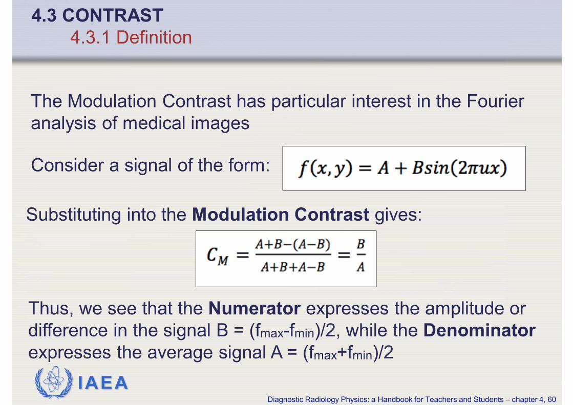


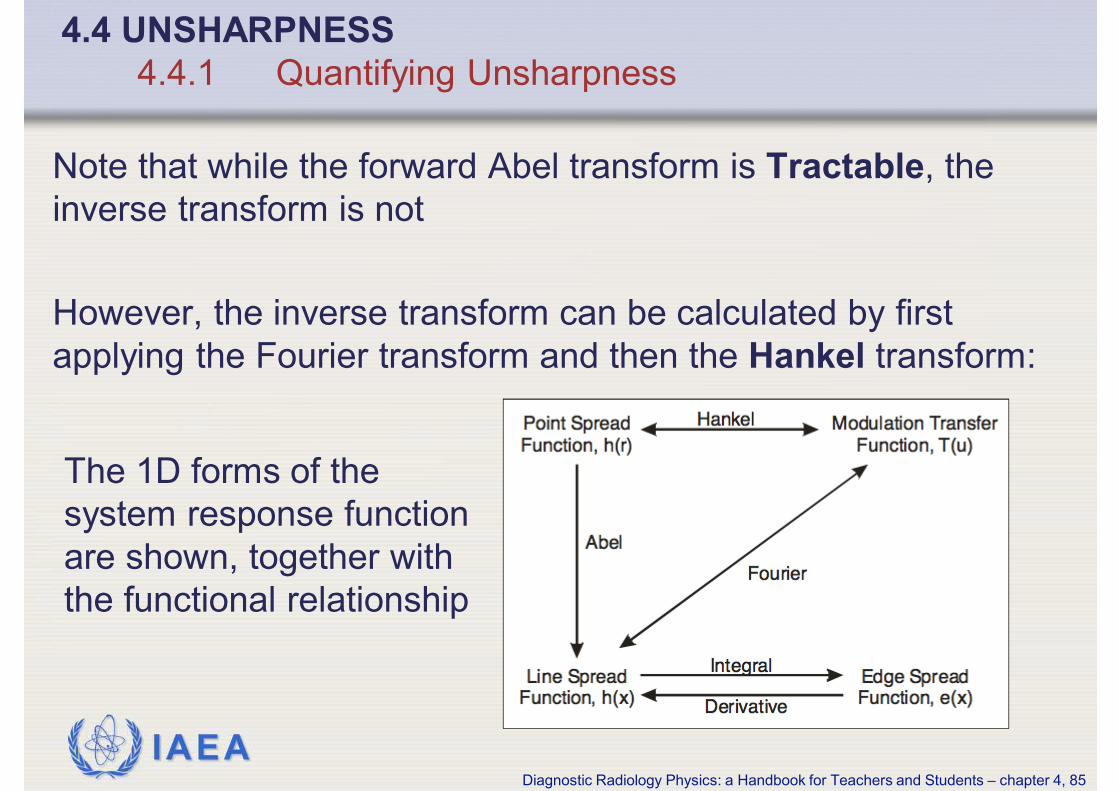


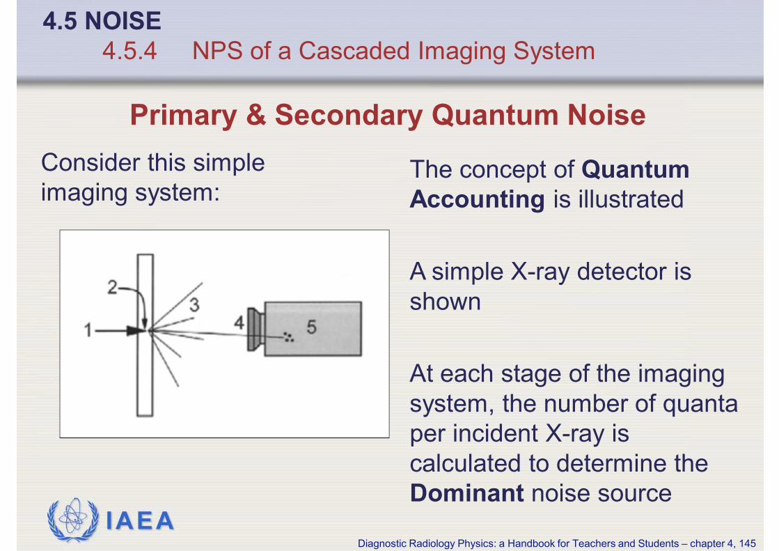


![University of Denvermathfiles/preprints/nsm-math-preprint-1432.pdf · fidelity of teleportation through their unsharpness and ... paradoxes and problems [3] t uses Positive Operator](https://static.documents.pub/doc/80x56/5f0c9cf37e708231d4364604/university-of-denver-mathfilespreprintsnsm-math-preprint-1432pdf-fidelity-of.jpg)


