Chapter 4Probability

4-1 Overview

4-2 Fundamentals

4-3 Addition Rule

4-4 Multiplication Rule: Basics

4-5 Multiplication Rule: Complements and Conditional Probability

4-6 Probabilities Through Simulations

4-7 Counting

Created by Tom Wegleitner, Centreville, Virginia

Section 4-1Overview

Overview

Rare Event Rule for Inferential Statistics:

If, under a given assumption, the probability of a particular observed event is extremely small, we conclude that the assumption is probably not correct.

Statisticians use the rare event rule for inferential statistics.

Created by Tom Wegleitner, Centreville, Virginia

Section 4-2 Fundamentals

Key Concept

This section introduces the basic concept of the probability of an event. Three different methods for finding probability values will be presented.

The most important objective of this section is to learn how to interpret probability values.

Definitions

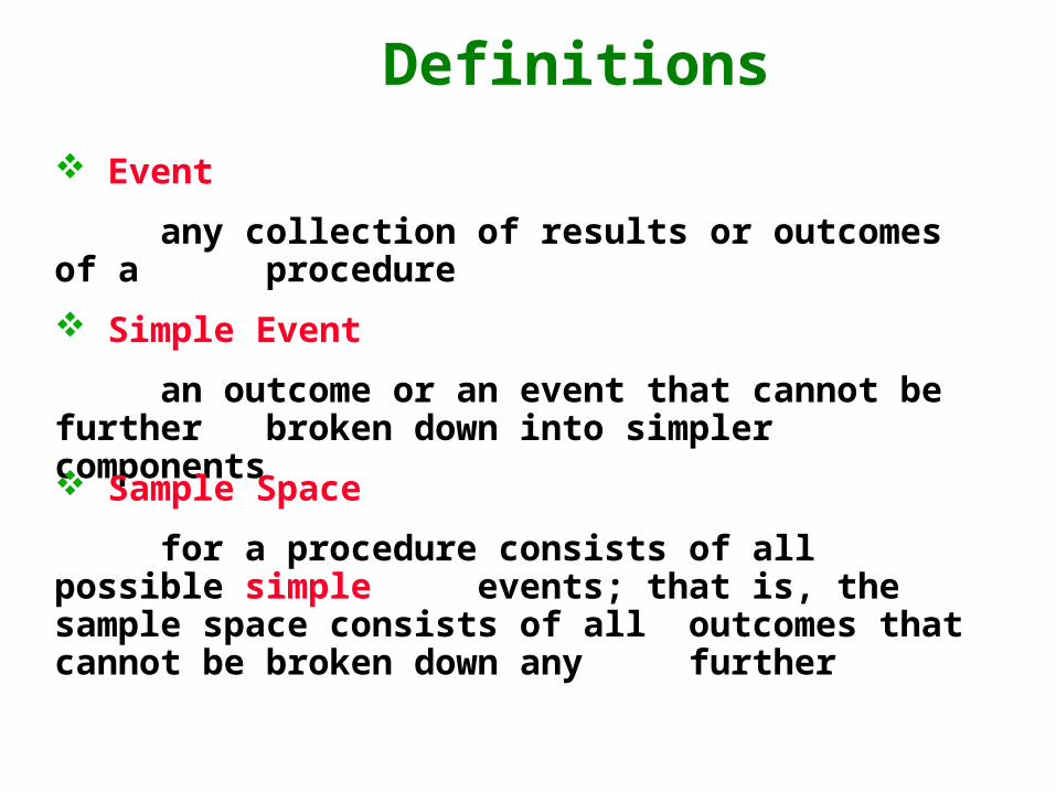
Event

any collection of results or outcomes of a procedure

Simple Event

an outcome or an event that cannot be further broken down into simpler components

Sample Space

for a procedure consists of all possible simple events; that is, the sample space consists of all outcomes that cannot be broken down any

further

Notation for Probabilities

P - denotes a probability.

A, B, and C - denote specific events.

P (A) - denotes the probability of event A occurring.

Basic Rules for Computing Probability

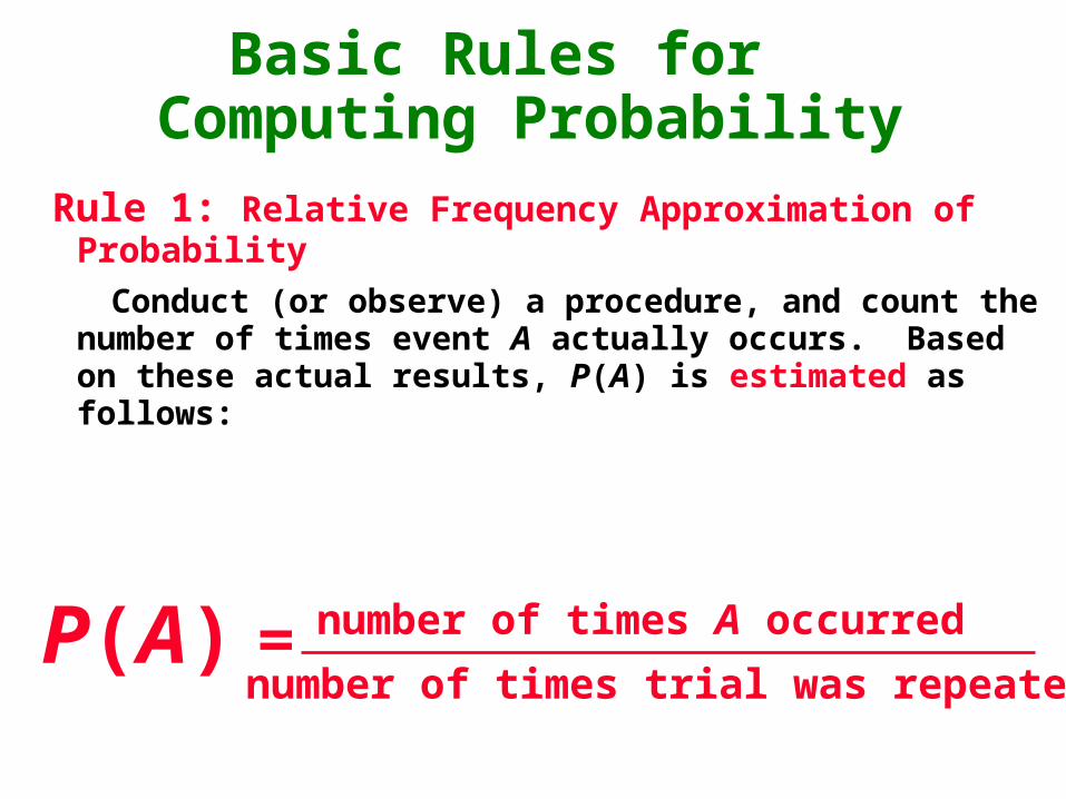
Rule 1: Relative Frequency Approximation of Probability

Conduct (or observe) a procedure, and count the number of times event A actually occurs. Based on these actual results, P(A) is estimated as follows:

P(A) = number of times A occurred

number of times trial was repeated

Basic Rules for Computing Probability - cont

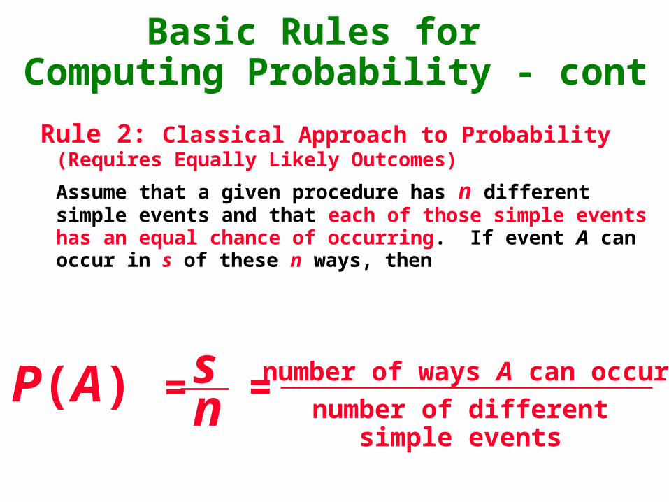
Rule 2: Classical Approach to Probability (Requires Equally Likely Outcomes)

Assume that a given procedure has n different simple events and that each of those simple events has an equal chance of occurring. If event A can occur in s of these n ways, then

P(A) = number of ways A can occur

number of different simple events

sn =

Basic Rules for Computing Probability - cont

Rule 3: Subjective Probabilities

P(A), the probability of event A, is estimated

by using knowledge of the relevant

circumstances.

Law of Large Numbers

As a procedure is repeated again and again, the relative frequency probability (from Rule 1) of an event tends to approach the actual probability.

Probability Limits

The probability of an event that is certain to occur is 1.

The probability of an impossible event is 0.

For any event A, the probability of A is between 0 and 1 inclusive. That is, 0 P(A) 1.

Possible Values for Probabilities

Definition

The complement of event A, denoted by

A, consists of all outcomes in which the

event A does not occur.

Rounding Off Probabilities

When expressing the value of a probability, either give the exact fraction or decimal or round off final decimal results to three significant digits. (Suggestion: When the probability is not a simple fraction such as 2/3 or 5/9, express it as a decimal so that the number can be better understood.)

Definitions

The actual odds against event A occurring are the ratio P(A)/P(A), usually expressed in the form of a:b (or “a to b”), where a and b are integers having no common factors.

The actual odds in favor of event A occurring are the reciprocal of the actual odds against the event. If the odds against A are a:b, then the odds in favor of A are b:a.

The payoff odds against event A represent the ratio of the net profit (if you win) to the amount bet.

payoff odds against event A = (net profit) : (amount bet)

Recap

In this section we have discussed:

Rare event rule for inferential statistics.

Probability rules.

Law of large numbers.

Complementary events.

Rounding off probabilities.

Odds.

Created by Tom Wegleitner, Centreville, Virginia

Section 4-3 Addition Rule

Key Concept

The main objective of this section is to present the addition rule as a device for finding probabilities that can be expressed as P(A or B), the probability that either event A occurs or event B occurs (or they both occur) as the single outcome of the procedure.

Compound Event any event combining 2 or more simple events

Definition

Notation

P(A or B) = P (in a single trial, event A occurs or event B occurs or they both occur)

When finding the probability that event A occurs or event B occurs, find the total number of ways A can occur and the number of ways B can occur, but find the total in such a way that no outcome is counted more than once.

General Rule for a Compound Event

Compound Event

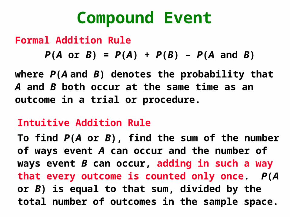
Intuitive Addition Rule

To find P(A or B), find the sum of the number of ways event A can occur and the number of ways event B can occur, adding in such a way that every outcome is counted only once. P(A or B) is equal to that sum, divided by the total number of outcomes in the sample space.

Formal Addition Rule

P(A or B) = P(A) + P(B) – P(A and B)

where P(A and B) denotes the probability that A and B both occur at the same time as an outcome in a trial or procedure.

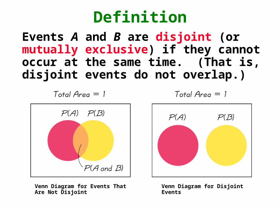
DefinitionEvents A and B are disjoint (or mutually exclusive) if they cannot occur at the same time. (That is, disjoint events do not overlap.)

Venn Diagram for Events That Are Not Disjoint

Venn Diagram for Disjoint Events

Complementary Events

P(A) and P(A)are disjoint

It is impossible for an event and its complement to occur at the same time.

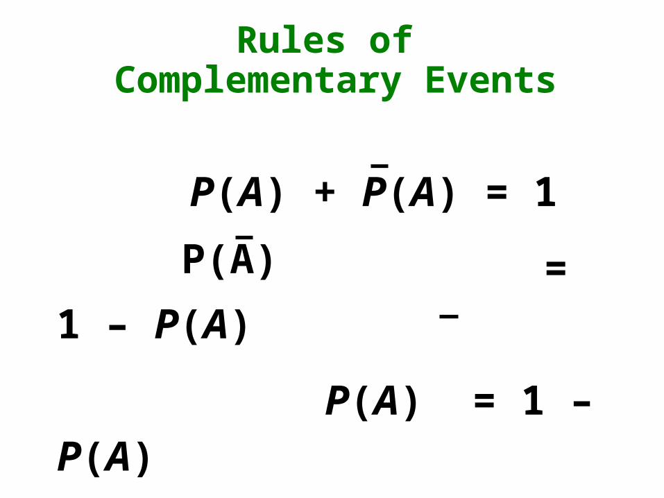
Rules of Complementary Events

P(A) + P(A) = 1

= 1 – P(A)

P(A) = 1 – P(A)

P(A)

Venn Diagram for the Complement of Event A

Recap

In this section we have discussed:

Compound events.

Formal addition rule.

Intuitive addition rule.

Disjoint events.

Complementary events.

Created by Tom Wegleitner, Centreville, Virginia

Section 4-4 Multiplication Rule:

Basics

Key Concept

If the outcome of the first event A somehow affects the probability of the second event B, it is important to adjust the probability of B to reflect the occurrence of event A.

The rule for finding P(A and B) is called the multiplication rule.

Notation

P(A and B) =

P(event A occurs in a first trial and

event B occurs in a second trial)

Tree DiagramsA tree diagram is a picture of the possible outcomes of a procedure, shown as line segments emanating from one starting point. These diagrams are helpful if the number of possibilities is not too large.

This figure summarizes the possible outcomes for a true/false followed by a multiple choice question.

Note that there are 10 possible combinations.

Key Point – Conditional Probability

The probability for the second event B should take into account the fact that the first event A has already occurred.

Notation for Conditional Probability

P(B A) represents the probability of event B occurring after it is assumed that event A has already occurred (read B A as “B given A.”)

Definitions

Independent Events

Two events A and B are independent if the occurrence of one does not affect the probability of the occurrence of the other. (Several events are similarly independent if the occurrence of any does not affect the probabilities of occurrence of the others.) If A and B are not independent, they are said to be dependent.

Formal Multiplication Rule

P(A and B) = P(A) • P(B A)

Note that if A and B are independent events, P(B A) is really the same as P(B).

Intuitive Multiplication Rule

When finding the probability that event A occurs in one trial and event B occurs in the next trial, multiply the probability of event A by the probability of event B, but be sure that the probability of event B takes into account the previous occurrence of event A.

Applying the Multiplication Rule

Small Samples from Large Populations

If a sample size is no more than 5% of the size of the population, treat the selections as being independent (even if the selections are made without replacement, so they are technically dependent).

Summary of Fundamentals

In the addition rule, the word “or” in P(A or B) suggests addition. Add P(A) and P(B), being careful to add in such a way that every outcome is counted only once.

In the multiplication rule, the word “and” in P(A and B) suggests multiplication. Multiply P(A) and P(B),

but be sure that the probability of event B takes into account the previous occurrence of event A.

Recap

In this section we have discussed:

Notation for P(A and B).

Notation for conditional probability.

Independent events.

Formal and intuitive multiplication rules.

Tree diagrams.

Created by Tom Wegleitner, Centreville, Virginia

Section 4-5 Multiplication Rule:Complements and

Conditional Probability

Key Concept

In this section we look at the probability of getting at least one of some specified event; and the concept of conditional probability which is the probability of an event given the additional information that some other event has already occurred.

Complements: The Probability of “At Least One”

The complement of getting at least one item of a particular type is that you

get no items of that type.

“At least one” is equivalent to “one or more.”

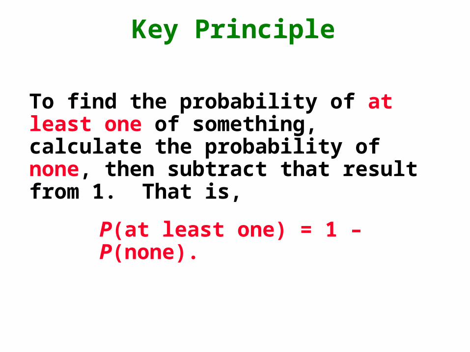
Key Principle

To find the probability of at least one of something, calculate the probability of none, then subtract that result from 1. That is,

P(at least one) = 1 – P(none).

DefinitionA conditional probability of an event is a probability obtained with the additional information that some other event has already occurred. P(B A) denotes the conditional probability of event B occurring, given that event A has already occurred, and it can be found by dividing the probability of events A and B both occurring by the probability of event A:

P(B A) = P(A and B)

P(A)

Intuitive Approach to Conditional Probability

The conditional probability of B given A can be found by assuming that event A has occurred and, working under that assumption, calculating the probability that event B will occur.

Recap

In this section we have discussed:

Concept of “at least one.”

Conditional probability.

Intuitive approach to conditional probability.

Created by Tom Wegleitner, Centreville, Virginia

Section 4-6Probabilities Through

Simulations

Key Concept

In this section we introduce a very different approach for finding probabilities that can overcome much of the difficulty encountered with the formal methods discussed in the preceding sections of this chapter.

Definition

A simulation of a procedure is a process that behaves the same way as the procedure, so that similar results are produced.

Simulation Example

Gender Selection When testing techniques of gender selection, medical researchers need to know probability values of different outcomes, such as the probability of getting at least 60 girls among 100 children. Assuming that male and female births are equally likely, describe a simulation that results in genders of 100 newborn babies.

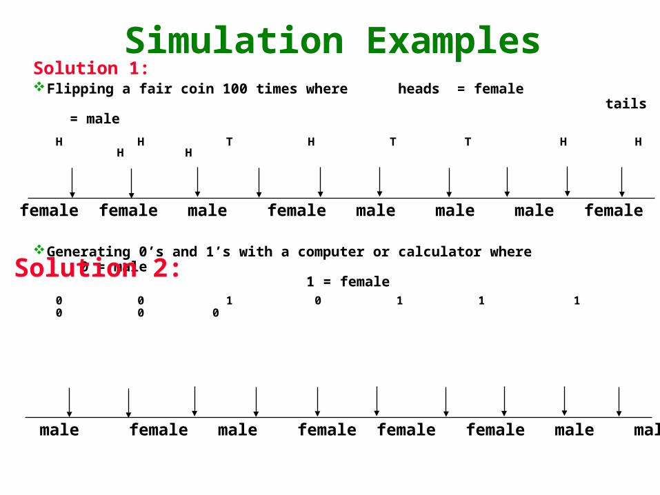
Simulation ExamplesSolution 1:Flipping a fair coin 100 times where heads = female and

tails = male

H H T H T T H H H H

Generating 0’s and 1’s with a computer or calculator where 0 = male

1 = female0 0 1 0 1 1 1 0 0 0

male male female male female female female male male male

female female male female male male male female female female

Solution 2:

Random Numbers

In many experiments, random numbers are used in the simulation of naturally occurring events. Below are some ways to generate random numbers.

A table of random of digits

Minitab

Excel

TI-83 Plus calculator

STATDISK

Random Numbers - cont Minitab STATDISK

Random Numbers - cont Excel TI-83 Plus calculator

Recap

In this section we have discussed:

The definition of a simulation.

Ways to generate random numbers.

How to create a simulation.

Created by Tom Wegleitner, Centreville, Virginia

Section 4-7Counting

Key Concept

In many probability problems, the big obstacle is finding the total number of outcomes, and this section presents several methods for finding such numbers without directly listing and counting the possibilities.

Fundamental Counting Rule

For a sequence of two events in which the first event can occur m ways and the second event can occur n ways, the events together can occur a total of m n ways.

Notation

The factorial symbol ! denotes the product of decreasing positive whole numbers.

For example,

4! 4 3 2 1 24.

By special definition, 0! = 1.

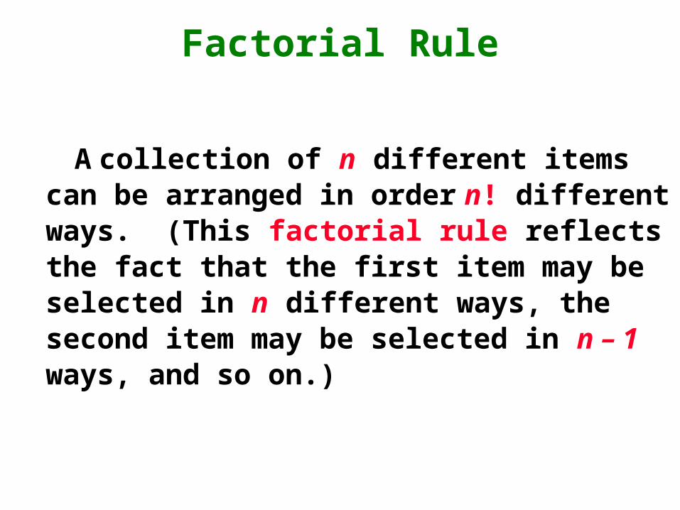
A collection of n different items can be arranged in order n! different ways. (This factorial rule reflects the fact that the first item may be selected in n different ways, the second item may be selected in n – 1 ways, and so on.)

Factorial Rule

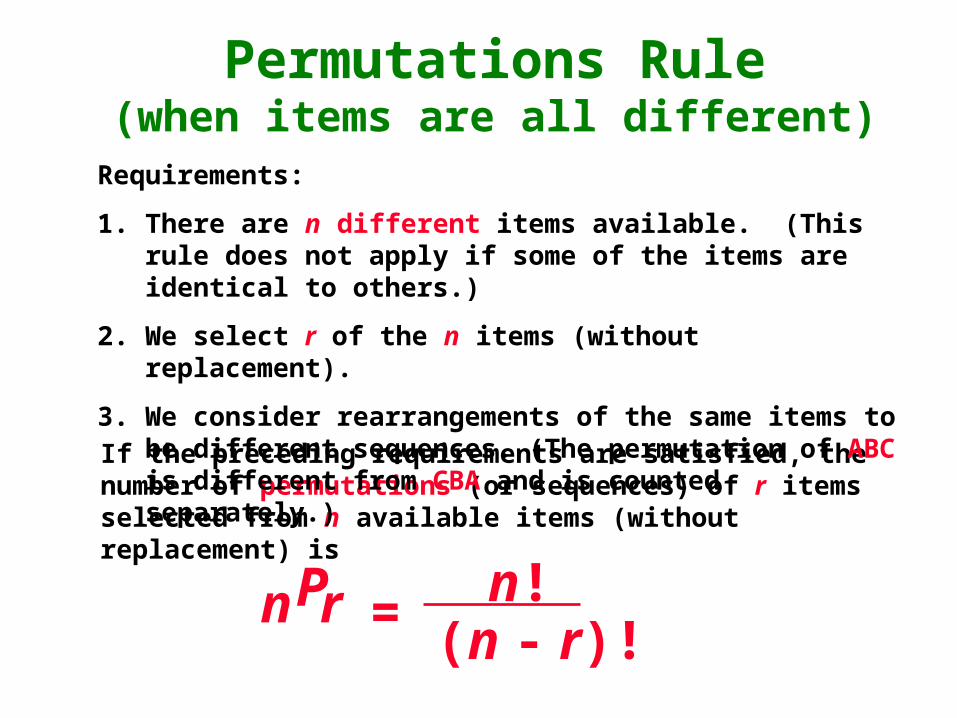
Permutations Rule(when items are all different)

(n - r)!n rP = n!

If the preceding requirements are satisfied, the number of permutations (or sequences) of r items selected from n available items (without replacement) is

Requirements:

1. There are n different items available. (This rule does not apply if some of the items are identical to others.)

2. We select r of the n items (without replacement).

3. We consider rearrangements of the same items to be different sequences. (The permutation of ABC is different from CBA and is counted separately.)

Permutations Rule(when some items are identical to others)

n1! . n2! .. . . . . . . nk! n!

If the preceding requirements are satisfied, and if there are n1 alike, n2 alike, . . . nk alike, the number of permutations (or sequences) of all items selected without replacement is

Requirements:

1. There are n items available, and some items are identical to others.

2. We select all of the n items (without replacement).

3. We consider rearrangements of distinct items to be different sequences.

(n - r )! r!n!

nCr =

Combinations Rule

If the preceding requirements are satisfied, the number of combinations of r items selected from n different items is

Requirements:

1. There are n different items available.

2. We select r of the n items (without replacement).

3. We consider rearrangements of the same items to be the same. (The combination of ABC is the same as CBA.)

When different orderings of the same items are to be counted separately, we have a permutation problem, but when different orderings are not to be counted separately, we have a combination problem.

Permutations versus Combinations

Recap

In this section we have discussed:

The fundamental counting rule.

The permutations rule (when items are all different).

The permutations rule (when some items are identical to others).

The combinations rule.

The factorial rule.