Chapter 4: RF/Microwave interaction and beam loading in SRF cavity 4.1 RF field in SRF cavity 4.2 Beam loading 4.3 Dynamic detuning (microphonics, Lorentz force detuning, etc) 4.4 Basics on RF control -develop equivalent circuit for rf system, cavity and beam -develop equations for steady state and transient -develop concept for the LLRF control
Transcript
Chapter 4:
RF/Microwave interaction and beam loading in SRF cavity
4.1 RF field in SRF cavity
4.2 Beam loading
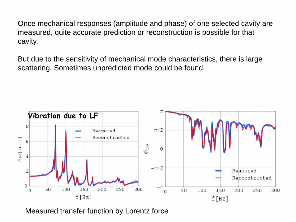
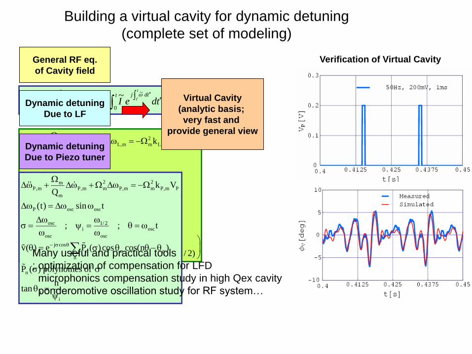
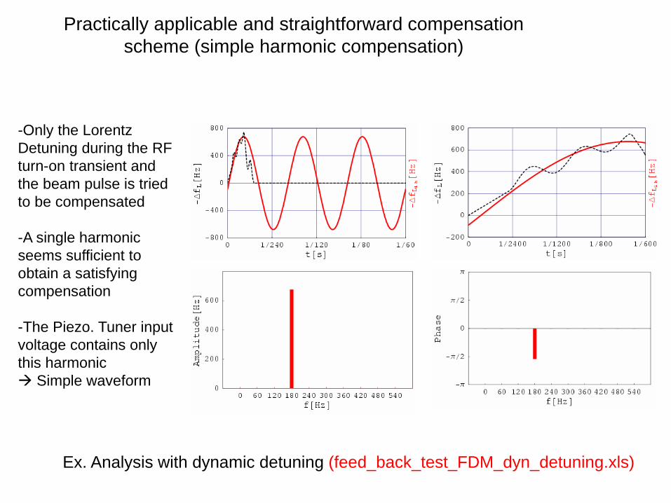
4.3 Dynamic detuning (microphonics, Lorentz force detuning, etc)
4.4 Basics on RF control
-develop equivalent circuit for rf system, cavity and beam
-develop equations for steady state and transient
-develop concept for the LLRF control
RF circuit modeling
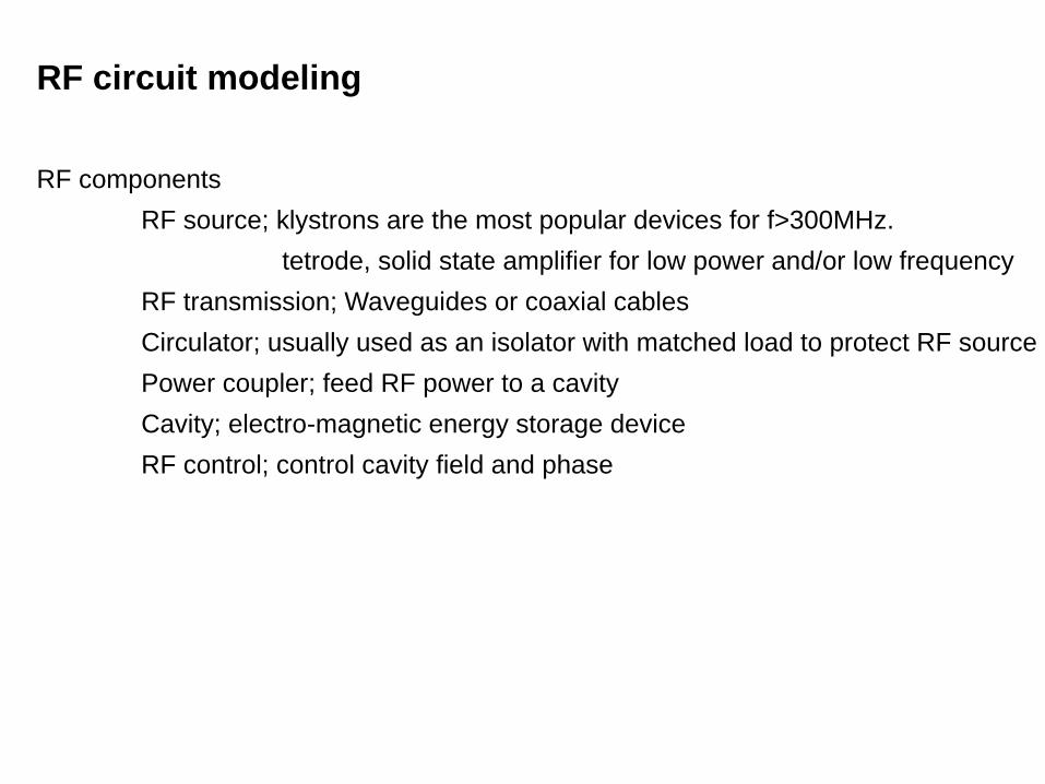
RF components
RF source; klystrons are the most popular devices for f>300MHz.
tetrode, solid state amplifier for low power and/or low frequency
RF transmission; Waveguides or coaxial cables
Circulator; usually used as an isolator with matched load to protect RF source
Power coupler; feed RF power to a cavity
Cavity; electro-magnetic energy storage device
RF control; control cavity field and phase
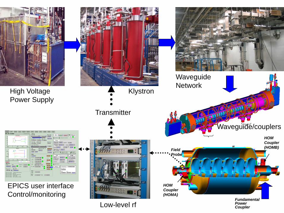
Fundamental Power Coupler
HOM
Coupler
(HOMB)
HOM
Coupler
(HOMA)
Field
Probe
High Voltage
Power Supply
Klystron
Waveguide
Network
Waveguide/couplers
Low-level rf
EPICS user interface
Control/monitoring
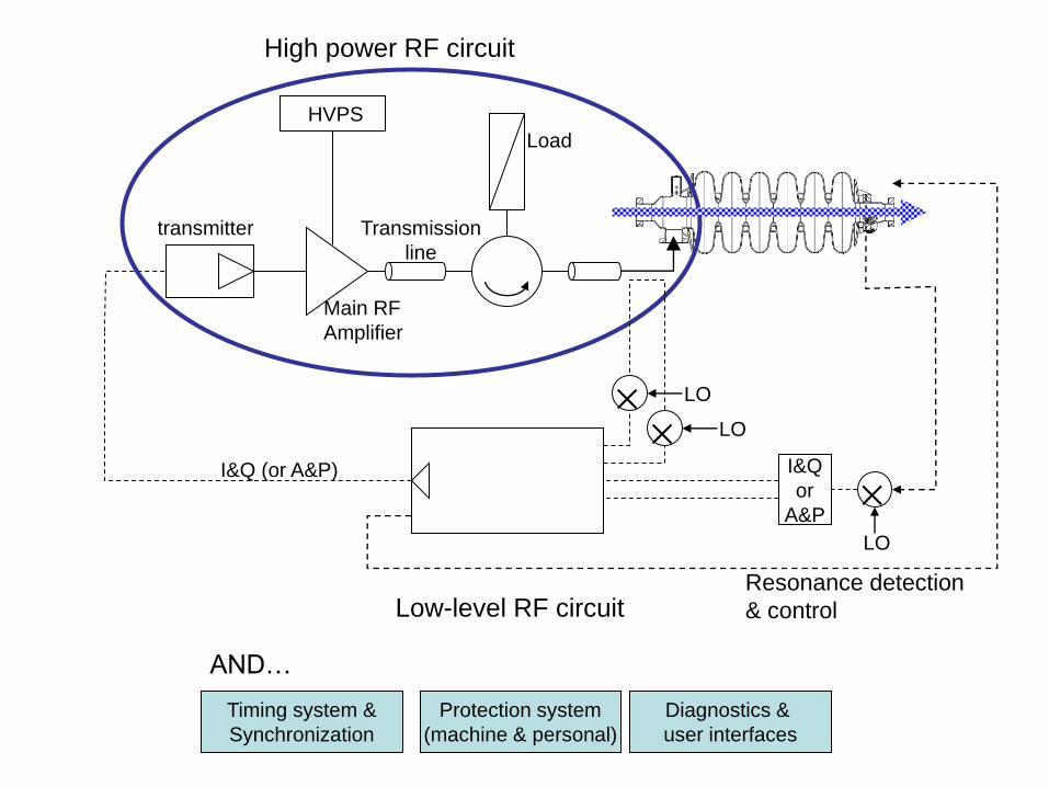
Transmitter
HVPS
High power RF circuit
Low-level RF circuit
Main RF
Amplifier
Transmission
line
LO
LO
LO
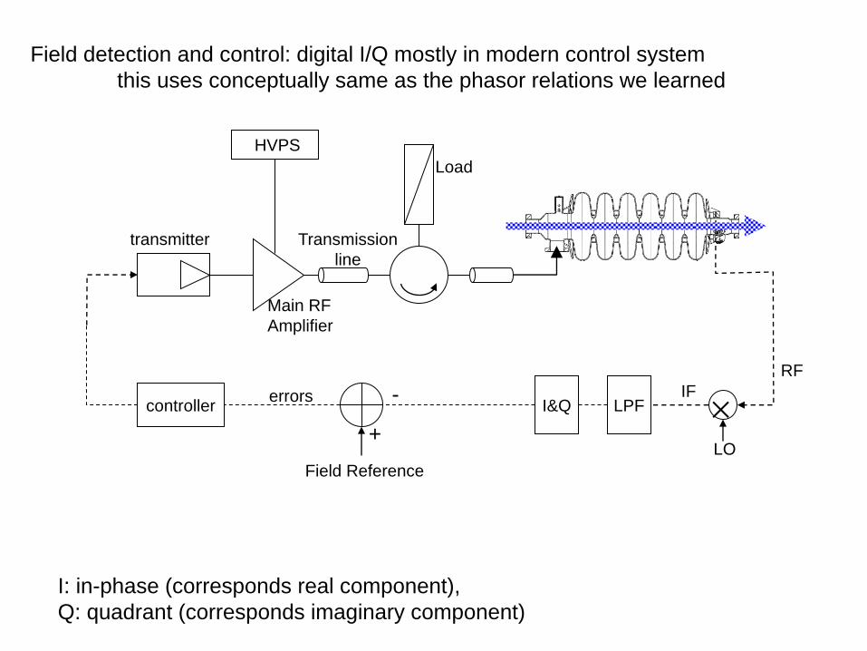
I&Q
or
A&P
I&Q (or A&P)
Timing system &
Synchronization
transmitter
AND…
Protection system
(machine & personal)
Diagnostics &
user interfaces
Load
Resonance detection
& control
~
Main RF
Amplifier
Transmission
line
First, main high power RF circuit and cavity responses without beam.
Equivalent circuit (will use effective quantities for the modeling)
Dummy
Load
Le Ce re
Va
~ Beam, Ib
Z0 1:n
gI
Due to the circulator, this is not an exactly equivalent for generator current.
So introduced
gI twice of equivalent generator current.
Power coupler
Circulator
Transmission
line
(with beam later on)
Covert the model to the cavity side
~ Le Ce re
Va
~ Beam, Ib
n
II
g
g
Zext’=
n2Z0T2
Le Ce re
Va
ΩTR
P
V
P
TV
P
TLEr
W 2R
V
R
V
r
TV
r
V
2r
VP
2
sh
c
2
a
c
2
0
c
2
0sh
2
0
sh
2
0
sh
2
0
sh
2
a
e
2
ac
defined in Chap. 2
L C R
V0
~ L C R
V0
n
II
g
g
Zext=
n2Z0
Remember that equivalent circuit
parameters are defined by
references (V0, Va).
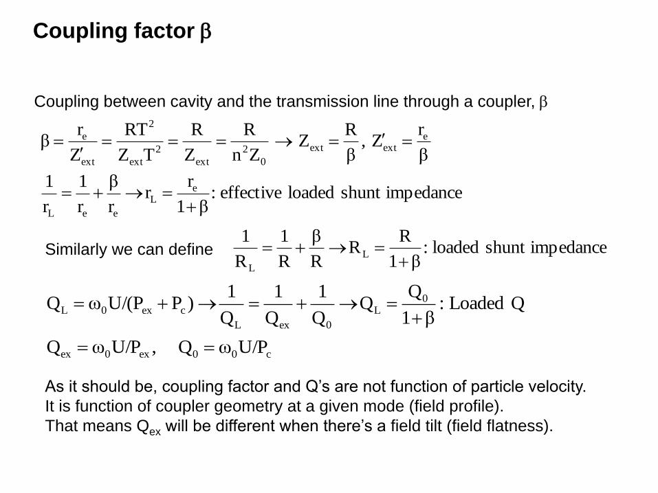
Coupling between cavity and the transmission line through a coupler, b
β
rZ,
β
RZ
Zn
R
Z
R
TZ
RT
Z
rβ e
extext
0
2
ext
2
ext
2
ext
e
Coupling factor b
,U/PωQ ex0ex c00 U/PωQ
impedanceshuntloadedeffective:β1
rr
r
β
r
1
r
1 eL
eeL
QLoaded:β1
QQ
Q
1
Q
1
Q
1)PU/(PωQ 0
L
0exL
cex0L
As it should be, coupling factor and Q’s are not function of particle velocity.
It is function of coupler geometry at a given mode (field profile).
That means Qex will be different when there’s a field tilt (field flatness).
impedanceshuntloaded:β1
RR
R
β
R
1
R
1L
L Similarly we can define
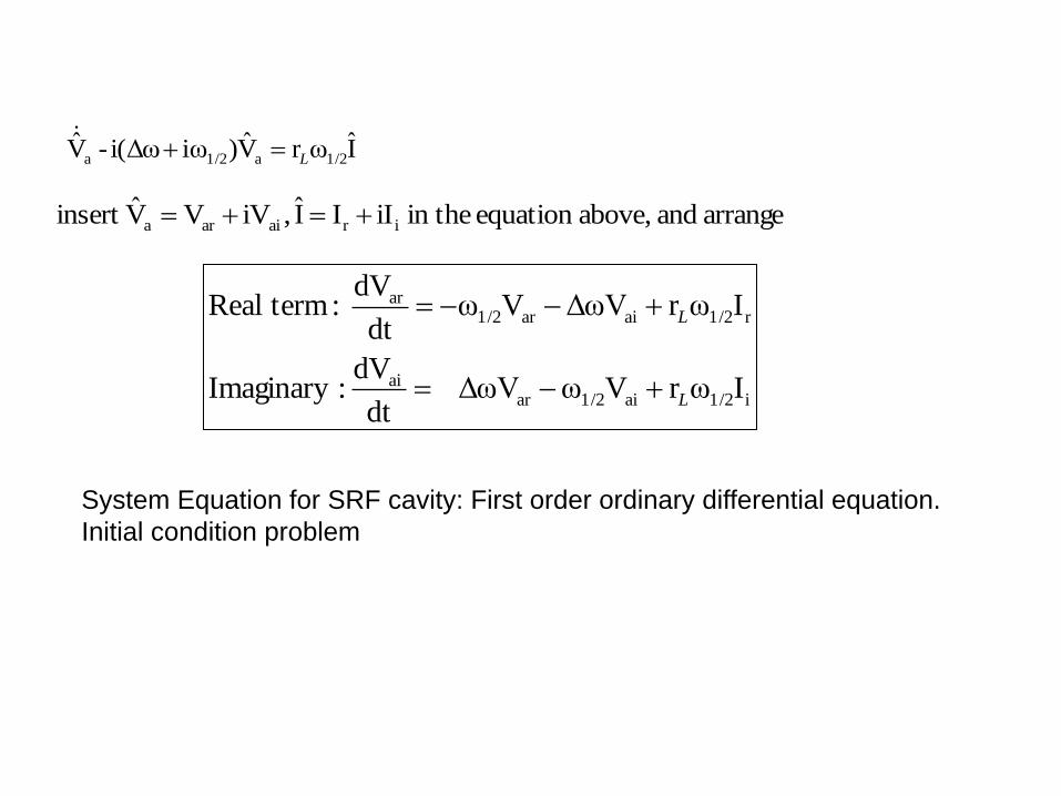
Governing equation for RF field in a cavity
~ Le Ce
Va
gI rL
IrL ILe ICe
geLrC LeIIII
eaL
Lar
aeC
dt/L
/r
C
e
L
e
VI
VI
VI
g
e
a
ee
a
eL
aga
e
a
L
aeC
1
CL
1
Cr
1
L
1
r
1C IVVVIVVV
If we use the equivalent circuit with V0,
rL should be replaced with RL
We can eliminate non-practical parameters (Ce, Le, C, L) using the relations:
L0
0
L
e0
LLe0
L
2
a
2
ae
0
cex
0L CRω
Lω
R
Lω
rrCω
r
V
2
1
VC2
1
ωPP
UωQ
g
L
L0a
2
0a
L
0a
Q
rωω
Q
ωIVVV
g
L
L0a
2
0a
L
0a
Q
rωω
Q
ωIVVV
Steady state solution with RF only
Generator current is the only source generator induced voltage Vg=Va
Particular solution in steady state of second order differential equation
ψ)ti(ω
aa eV(t) Vtiω
gg eI(t) Iat
angledetuning:ψ
1 when δ,2Qf
Δf2Q
ω
ωω2Q
ω
ω
ω
ωQtanψ
0)Δfif,eIr(eIψtan1
reI
ω
ω
ω
ωQ1
r(t)
L
0
L
0
0L
0
0L
tiω
gL
ψ)ti(ω
g2
Lψ)ti(ω
g2
0
02
L
La
V
Typical damped driven oscillator equation
Phasor representation
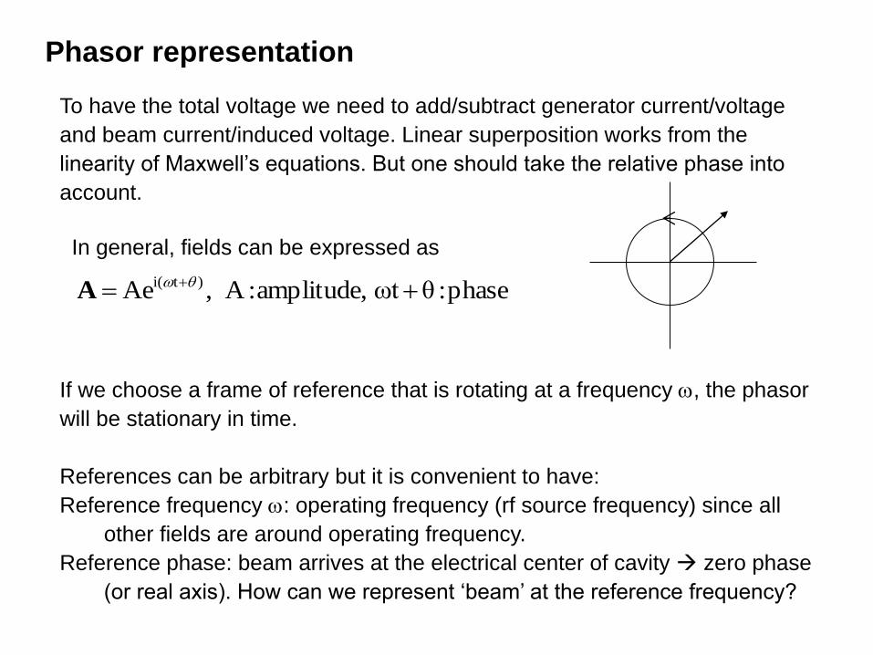
In general, fields can be expressed as
phase:θωtamplitude,:A,Ae )ti( A
To have the total voltage we need to add/subtract generator current/voltage
and beam current/induced voltage. Linear superposition works from the
linearity of Maxwell’s equations. But one should take the relative phase into
account.
If we choose a frame of reference that is rotating at a frequency , the phasor
will be stationary in time.
References can be arbitrary but it is convenient to have:
Reference frequency : operating frequency (rf source frequency) since all
other fields are around operating frequency.
Reference phase: beam arrives at the electrical center of cavity zero phase
(or real axis). How can we represent ‘beam’ at the reference frequency?
1
x
ψcosψtan1
1x
2
tiωiψ
gL
ψ)ti(ω
g2
La eecosψIreI
ψtan1
r(t)
V
common rotating term
relative phase
change due to
detuning
Amplitude
decrease
due to
detuning
iψshiψeiψ
L
g
atot ecosψ
β)2(1
recosψ
β1
recosψr
(t)
(t)Z
I
V
Total impedance of the equivalent model including detuning without beam
0.00E+00
2.00E-01
4.00E-01
6.00E-01
8.00E-01
1.00E+00
1.20E+00
-6000 -4000 -2000 0 2000 4000 6000-1.00E+02
-8.00E+01
-6.00E+01
-4.00E+01
-2.00E+01
0.00E+00
2.00E+01
4.00E+01
6.00E+01
8.00E+01
1.00E+02
-6000 -4000 -2000 0 2000 4000 6000
Va/(rLIg)
f0-f
Ex) QL=7105, f=805 MHz
plot the normalized Va and the detuning angle as a function of cavity detuning
f0-f
Bandwidth at -3bB: 10log10(P/Pref) for power, 20log10(V/Vref) for voltage
20log10(1/sqrt(2))=-3.01 =/4
Half width at -3dB: 1/2= 0/(2QL)=2575 Hz in this example
(time constant of loaded cavity)=1/1/2=2QL/0=277s
f, f/f=QL
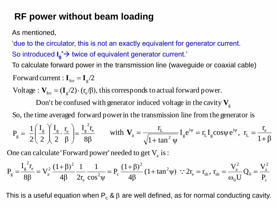
RF power without beam loading
As mentioned,
‘due to the circulator, this is not an exactly equivalent for generator current.
So introduced Ig* twice of equivalent generator current.’
To calculate forward power in the transmission line (waveguide or coaxial cable)
8β
rI
β
r
2
I
2
I
2
1P
isgenerator thefrom lineion transmissin thepower forward averaged time theSo,
cavity in the voltageinducedgenerator with confused bet Don'
power. forward actual toscorrespond thisβ),/(r/2)(:Voltage
/2:current Forward
e
2
gegg
g
g
egfor
gfor
V
IV
II
β1
rr,ecosψIreI
ψtan1
rwith e
L
iψ
gL
iψ
g2
La
V
c
2
a0
0
2
ashshe
22
c2
e
22
a
e
2
g
g
a
P
VQ
Uω
Vr,r2r ψ)tan(1
4β
β)(1P
ψcos
1
2r
1
4β
β)(1V
8β
rIP
:is Vget toneeded power' Forward' calculatecan One
This is a useful equation when Pc & b are well defined, as for normal conducting cavity.
loading) beamwithout ( ag VV
forV
refV
phasein,β2
1β
resonanceon voltageinducedgenerator :1β
rr
2β
r
rg,
for
ge
gLrg,
ge
for
V
V
IIV
IV
loading) beamwithout ( ag VV
rg,V forV
refV
rg,V
b>1 b<1
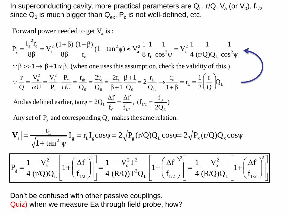
In superconducting cavity, more practical parameters are QL, r/Q, Va (or V0), f1/2
since Q0 is much bigger than Qex, Pc is not well-defined, etc.
ψcos
1
(r/Q)Q
1
4
1V
ψcos
1
r
1
8
1Vψ)tan(1
r
β)(1
8β
β)(1V
8β
rIP
:is Vget toneededpower Forward
2
L
2
a2
L
2
a
2
e
2
a
e
2
g
g
a
relation. same themakes Q ingcorrespond and P ofset Any
)2Q
f(f ,
f
Δf
f
Δf2Q tanψearlier, defined asAnd
QQ
r
2
1r
β1
r
Q
r2
Q
1β
1β
2r
Q
2r
Q
r
Uω
P
P
V
Uω
V
Q
r
this.)of validity check the ,assumption thisuses one(when β.1β 1β
xx
L
01/2
1/20
L
LLe
L
L
0
e
0
e
0
shc
c
2
a
2
a
2
1/2L
2
o
2
1/2L
2
22
o
2
1/2L
2
ag
f
Δf1
(R/Q)Q
V
4
1
f
Δf1
Q(R/Q)T
TV
4
1
f
Δf1
(r/Q)Q
V
4
1P
cosψ(r/Q)QP2cosψ(r/Q)QP2cosψIrIψtan1
rxxLggLg
2
La
V
Don’t be confused with other passive couplings.
Quiz) when we measure Ea through field probe, how?
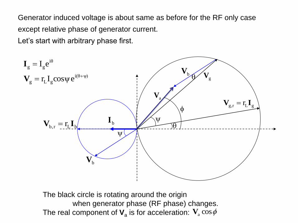
gV
resonanceonissystemthewhen
fieldcavityinducedGeneratorr gLrg, IV forV
refV
When b >>1
reffor
gL
ge
ge
for2
r
1)2(β
r
2β
r
VV
IIIV
iψ
gLag ecosψIrloading) beamwithout ( VV
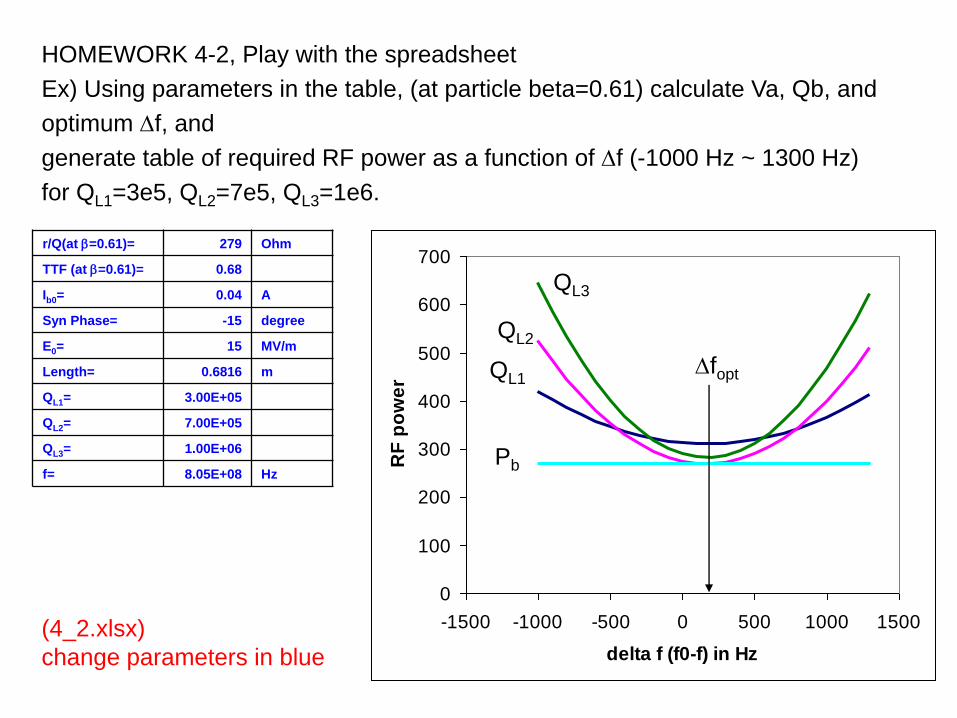
HOMEWORK 4-1
for f=805 MHz, Ea=10MV/m, L=0.68m, r/Q=279, and
QL=7105, QL=1106, QL=2106,
1. Plot required forward power as a function of detuning (-500 Hz~500 Hz)
using spreadsheet 4_1.xlsx
2. If Q0=11010, What is cavity wall loss, Pc? What does that mean?
Equivalent beam in a RF circuit model
Micro-pulse Bunch spacing=Tb
RF frequency/n
When we say ‘Beam current’, it is an time averaged DC current.
Ex) Ib0=40 mA CW beam at bunch spacing 402.5 MHz
Tb=1/402.5 MHz~2.5ns,
Q (charge per bunch)=Ib0 (C/s) x Tb (s)=0.04 x 2.5e-9 = 100 pC
Temporal distribution of beam can be described by a Gaussian distribution with