Chapter 5 Experimentally Estimating Phase Response Curves...

Chapter 5Experimentally Estimating Phase ResponseCurves of Neurons: Theoretical and PracticalIssues

Theoden Netoff, Michael A. Schwemmer, and Timothy J. Lewis

Abstract Phase response curves (PRCs) characterize response properties ofoscillating neurons to pulsetile input and are useful for linking the dynamics ofindividual neurons to network dynamics. PRCs can be easily computed for modelneurons. PRCs can be also measured for real neurons, but there are many issues thatcomplicate this process. Most of these complications arise from the fact that neuronsare noisy on several time-scales. There is considerable amount of variation (jitter)in the inter-spike intervals of “periodically” firing neurons. Furthermore, neuronalfiring is not stationary on the time scales on which PRCs are usually measured.Other issues include determining the appropriate stimuli to use and how long towait between stimuli.

In this chapter, we consider many of the complicating factors that arise whengenerating PRCs for real neurons or “realistic” model neurons. We discuss issuesconcerning the stimulus waveforms used to generate the PRC and ways to dealwith the effects of slow time-scale processes (e.g. spike frequency adaption).We also address issues that are present during PRC data acquisition and discussfitting “noisy” PRC data to extract the underlying PRC and quantify the stochasticvariation of the phase responses. Finally, we describe an alternative method togenerate PRCs using small amplitude white noise stimuli.

T. Netoff (�)Department of Biomedical Engineering, University of Minnesota, Minneapolis, MN 55455, USAe-mail: [email protected]

M.A. Schwemmer • T.J. LewisDepartment of Mathematics, University of California, Davis, CA 95616, USAe-mail: [email protected]; [email protected]

N.W. Schultheiss et al. (eds.), Phase Response Curves in Neuroscience: Theory,Experiment, and Analysis, Springer Series in Computational Neuroscience 6,DOI 10.1007/978-1-4614-0739-3 5, © Springer Science+Business Media, LLC 2012

95

96 T. Netoff et al.

1 Introduction

A phase response curve (PRC) quantifies the response of a periodically firing neuronto an external stimulus (Fig. 5.1). More specifically, it measures the phase shiftof the oscillating neuron as a function of the phase that a stimulus is delivered.The task of generating a PRC for a real neuron seems straightforward: (1) If theneuron is not oscillating, then inject a constant current or apply a neuromodulatorto make the neuron fire with the desired period. (2) Deliver a pulsatile stimulus at aparticular phase in the neuron’s periodic cycle, and measure the subsequent change

Fig. 5.1 PRC measured froma cortical pyramidal neuron.Top panel: voltage from anunperturbed periodicallyfiring neuron (solid line);voltage from neuronstimulated with synapticconductance near the end ofthe cycle, resulting in anadvance of the spike fromnormal period (dash-dottedline); voltage from a neuronstimulated early in the cycle,resulting in slight delay ofspike (dotted line). Bottompanel: spike advancemeasured as a function of thephase of stimulation. Eachdot represents the response toa stimulus. Solid line is afunction fit to the raw data,estimating the PRC. Errorbars indicate the standarddeviation at each stimulusphase. The dashed line is thesecond order PRC, i.e. itindicates the effect of thesynaptic input at that phaseon the period following thestimulated period. Figureadapted from Netoffet al. 2005b

5 Experimentally Estimating Phase Response Curves of Neurons: Theoretical... 97

in timing of the next spike (Fig. 5.1 top panel). (3) Repeat these steps for manydifferent phases (Fig. 5.1 bottom panel). However, there are many subtle issues thatcomplicate this seemingly simple process when dealing with real neurons.

Many of the complicating factors in generating PRCs arise from the fact thatneurons are inherently noisy on several timescales. There is usually a considerableamount of variation in the interspike intervals of “periodically” firing neurons. Thisjitter in interspike intervals confounds the change in phase that is due to a stimulus.Furthermore, neuronal firing is typically not stationary over the timescales on whichPRCs are measured, and a PRC can change significantly with the firing rate of aneuron. Other important issues that need consideration when constructing PRCsarise from the inherent nonlinearities and slow timescale processes of neuronaldynamics. These issues include determining the appropriate stimuli and decidinghow long to wait between stimuli.

In this chapter, we will discuss many of the complicating factors that arise whengenerating PRCs for real neurons or “realistic” model neurons. In Sects. 2 and 3, wefocus on theoretical issues for which noise is not a factor. Section 2 addresses issuesaround the stimulus waveforms used to generate the PRC. Section 3 discusses theeffects of slow timescale processes, such as spike frequency adaption, on the phaseresponse properties of a neuron. In Sects. 4 and 5, we discuss issues that arise whenmeasuring PRCs in “real-world” noisy conditions. Section 4 deals with issues thatare present during data acquisition, and Sect. 5 discusses fitting “noisy” PRC datato extract the underlying PRC and quantifying the stochastic variation of the phaseresponses. Finally, in Sect. 6, we describe an alternative method to generate PRCsusing small amplitude white noise stimuli.

2 Choosing an Appropriate Stimulus

PRCs are often used to predict the phase-locking dynamics of coupled neurons,using either spike-time response curve (STRC) maps (e.g., (Canavier 2005; Netoffet al. 2005) also see Chap. 4) or the theory of weakly coupled oscillators (e.g.,(Ermentrout & Kopell 1991; Kuramoto 1984); also see Chaps. 1 and 2) as follows:

1. The STRC map approach can be used for networks in which synaptic inputs canbe moderately strong but must be sufficiently brief. The limiting assumption ofSTRC map approach is that the effect of any input to a neuron must be completebefore the next input arrives. In this case, the PRC can be used to predict thephase shift due to each synaptic input. Therefore, if one intends to use the STRCmap method to predict phase-locking behavior, then PRCs should be generatedusing a stimulus that approximates the synaptic input in the neuronal circuitunder study.

2. The theory of weakly coupled oscillators can be used for completely generalcoupling but the total coupling current incident on a neuron at any time must besufficiently small. The limiting assumption of this method is that the effects of the

98 T. Netoff et al.

inputs sum linearly, i.e., the neurons respond to input like a time-dependent linearoscillator. The infinitesimal PRC (iPRC), which is used in the theory of weaklycoupled oscillators, can be obtained from any PRC generated with sufficientlysmall perturbations (so long as the perturbation elicits a “measurable” response).Typically, current-based stimuli that approximate delta functions are used.

As indicated above, the choice of stimulus used to generate a PRC depends on theintended use of the PRC. It also depends on the need for realistic stimuli and easeof implementation. In this section, we will address some of the issues involved inchoosing an appropriate stimulus waveform to generate a PRC. For the case of smallamplitude stimuli, we will also describe the relationships between PRCs generatedwith different stimulus waveforms.

2.1 Stimulus Waveforms

2.1.1 Current-based Synaptic Input

Perhaps the simplest stimulus waveform used to measure a neuron’s PRC is a squarepulse of current. Square wave current stimuli are easy to implement in models andin a real neuron, using a waveform generator. A possible drawback is that squarewave pulses do not resemble synaptic conductances (however, see Sect. 2.2).

A current stimulus waveform that has a shape similar to realistic synaptic inputis an alpha function

Isyn.t/ D Smax1

�f � �r

�e� t

�f � e� t�r

�; t � 0;

where Smax controls the amplitude of the synaptic current, �f is the time constantthat controls the decay (“fall”) of the synaptic current, and �r is the time constantthat controls the rise time of the synaptic current. Here, t D 0 is the time at theonset of each synaptic input. Examples of alpha functions with different coefficientsare plotted in Fig. 5.2. The coefficients of the alpha function current stimulus canbe chosen in order to fit the postsynaptic potentials (PSPs) measured in neuronsof interest.1 In the neocortex, physiologically reasonable values for the synapticconductance time constants are �f � 1:8ms and �r � 1:4ms for fast excitatorysynapses and �f � 3:5ms and �r � 1:0ms for fast inhibitory synapses (Cruikshank,Lewis, & Connors 2007). The peak amplitude is synapse specific and depends on theresistance of the neuron. We usually adjust the amplitude of the synaptic current so

1The time constants of the synaptic currents will be faster than those for the PSP because the currentwaveform is filtered due to the RC properties neuronal membrane. To find the time constants ofthe synaptic currents, one can adjust these time constants until the current stimulus induces a PSPwaveform that adequately matches an actual PSP.


0 5 10 15 200

0.05

0.1

0.15

0.2

0.25

Time (msec)

Am

plitu

de (

AU

)

τs=6, τf=1

τs=4, τf=1

τs=6, τf=3

τs=4, τf=2

τs=2, τf=1

Fig. 5.2 Alpha function current stimuli plotted with different time constants and the same totalcurrent (in arbitrary units, AU)

that it elicits a PSP of �1mV in amplitude. Figure 5.3 shows PRCs generated usingan alpha function current stimulus with a positive Smax to simulate an excitatorysynaptic input (top) and a negative Smax to simulate an inhibitory synapse (bottom).

The shape of the PRC can be significantly affected by the shape of thestimulus waveform used to generate it. PRCs measured from the same neuronusing excitatory currents with different time constants are shown in Fig. 5.4. Asthe synaptic time constants increase, the PRC peak shifts down and to the left. Thisshift in the PRC is associated with changes in phase-locking of synaptically coupledneurons; simply by slowing the time constants of the synapses, it is possible fora network to transition from synchronous firing to asynchronous firing (Lewis &Rinzel 2003; Netoff et al. 2005; Van Vreeswijk, Abbott, & Ermentrout 1994).

The PRC can also be affected by the magnitude of the stimulus used to generateit. As shown in the example in Fig. 5.5, the peak of the PRC typically shifts up and tothe left as the magnitude of excitatory input increases. PRCs for inhibitory pulses aregenerally flipped compared to those for excitatory pulses, and the peak in the PRCtypically shifts down and to the right as the magnitude of inhibitory input increases.For sufficiently small input, the magnitude of the PRC scales approximately linearlywith the magnitude of the input. In fact, for sufficiently small input, the changes inthe PRC that occur due to changes in the stimulus waveform can be understoodin terms of a convolution of the stimulating current with the neuron’s so-calledinfinitesimal PRC. This will be described more fully in Sect. 2.2. Some of thechanges in the PRC that occur in response to changes of the stimuli with largemagnitudes follow the same trends found for small stimuli; however, other changesare more complicated and involve the nonlinear properties of neurons.

When stimulating a neuron, the maximum a neuron’s spike can be advanced isto the time of the stimulus. In other words, the spike cannot be advanced to a timebefore the stimulus was applied. Therefore, the spike advance is limited by causality.Often we plot the causality limit along with the PRC to show the maximal advance(as shown in Fig. 5.16). When plotting PRCs measured from neurons if the stimulus

100 T. Netoff et al.

0 1 2 3 4 5 6 7

−60

−40

−20

0

Time (msec)

Mem

bran

eV

olta

ge (

mV

)

0 0.2 0.4 0.6 0.8 10

0.02

0.04

phase

0 0.2 0.4 0.6 0.8 1phase

Pha

se a

dvan

ce

−0.06

−0.04

−0.02

0

Pha

se a

dvan

ce

Fig. 5.3 Phase response curves measured with alpha-function current stimuli: [top] voltage tracefrom neuron over one period [middle] excitatory stimuli, [bottom] inhibitory stimuli. Each plotdepicts the spike time advance, in proportion of the period, as a function of stimulus phase.Zero phase and a phase of 1 are defined as voltage crossing of �20mV. The INa C IK modelof Izhikevich (2007) was used to model neuronal dynamics with ISI D 15ms. The synapticparameters were �r D 0:25ms, �f D 0:5ms, and Smax D 0:04

was too strong much of the data will hug the causality limit for a significant portionof the phase. This indicates that the stimulus is eliciting an action potential at thesephases. If this is the case, we will drop the stimulus strength down. Because eachneuron we record has a different resistance, it is not possible to choose one stimulusamplitude that works for every cell. We often have to adjust the amplitude. If thestimulus amplitude is too weak, we find the PRC is indistinguishable from flat.

The line of causality can affect the estimate of the PRC as well. If the neuron isclose to the line of causality, it effectively truncates the noise around the PRC. PRCsmeasured using excitatory synaptic inputs are affected more by the line of causalitythan those measured with inhibitory synaptic inputs, where the effect is to generallydelay the next spike. In Chap. 7 of this book, it will be addressed how the truncationof the noise can affect the estimation of the PRC and how to correct for it.


0 0.1 0.2 0.3 0.4 0.5 0.6 0.7 0.8 0.9 10

0.01

0.02

0.03

0.04

0.05

0.06

Phase

Pha

se A

dvan

ce

τr=.25, τf=.5

τr=.5, τf=1

τr=.75, τf=1.5

τr=1, τf=2

Fig. 5.4 The shape of PRC changes with the shape of the stimulus waveform. Phase responsecurves are measured with alpha function excitatory current stimuli. Inset shows synaptic wave-forms as the rise time constants and falling time constants are varied. The INa C IK model ofIzhikevich (2007) was used to model neuronal dynamics with a period of 7.2 ms and Smax D 0:04

−0.15

−0.1

−0.05

0

0.05

0.1

0.15

phase

Pha

se a

dvan

ce Smax= 0.1

Smax= 0.06

Smax= 0.02

Smax= –0.02

Smax= –0.06

Smax= –0.1

0 0.1 0.2 0.3 0.4 0.5 0.6 0.7 0.8 0.9

Fig. 5.5 The shape of PRC changes with the magnitude of the stimulus waveform. Phase responsecurves are measured with alpha-function current stimuli. The INa CIK model of Izhikevich (2007)was used to model neuronal dynamics with ISI D 15ms. The synaptic time constants were �r D0:25ms and tf D 0:5ms


2.1.2 Conductance-based Synaptic Input

When a neurotransmitter is released by a presynaptic cell, it opens ion channels inthe postsynaptic cell, evoking a synaptic current carried by the flow of ions throughthe cell membrane. The synaptic current depends on the number of channels opened(i.e., the activated synaptic conductance) and the potential across the membrane. Tosimulate a more realistic “conductance-based” synapse, an alpha function can beused to describe the synaptic conductance waveform which is then multiplied bysynaptic driving force (the difference between the membrane potential V and thereversal potential of the synaptic current Esyn/ to calculate the synaptic current

Isyn.t/ D Gsyn.t/.Esyn � V.t//; t � 0;

where the synaptic conductance waveformGsyn.t/ is defined to be

Gsyn.t/ D gsyn1

�s � �f

�e� t

�s � e� t�f

�; t � 0:

The parameter gsyn scales the amplitude of the synaptic conductance. Note thatstimulating a neuron with a conductance waveform requires a closed loop feedbacksystem, called a dynamic clamp. The details of a dynamic clamp will be discussedSect. 4.1.

The synaptic reversal potential is calculated using the Nernst equation if thechannels only pass one ion, or the Goldman–Hodgkin–Katz equation if it passesmultiple ions (Hille 1992). Excitatory glutamatergic ion channels are cationic,passing some sodium and potassium ions, and therefore the associated excitatorysynaptic current reversal potential is usually set near 0 mV. Inhibitory GABAergicion channels pass mainly chloride or potassium ions, and therefore the associatedinhibitory synaptic reversal potential is usually set near �80mV. The time constantsfor synaptic conductances are very similar to those previously quoted for synapticcurrents.

In Fig. 5.6, the synaptic conductance profiles and corresponding current wave-forms for an excitatory synaptic conductance-based input are plotted for differentinput phases, as illustrated in the Golomb–Amitai model neuron (Golomb &Amitai 1997). As the neuron’s membrane potential changes over the cycle, so doesthe synaptic driving force. Thus, the synaptic current waveform will be differentfor different input phases. For this reason, a PRC measured with a conductance-based input will be different from a PRC measured using a stimulus with a fixedcurrent waveform. For excitatory conductance-based synaptic inputs, the inputcurrent can even reverse direction when the action potential passes through theexcitatory synaptic reversal potential. Differences between PRC generated withinhibitory conductance-based input current-based input are more pronounced thanfor excitatory input because the cell’s voltage between action potentials is muchcloser to the inhibitory reversal potential than for the excitatory reversal potential.This results in larger fractional changes of the driving force (and therefore inputcurrent) when compared to excitatory synapses.


Fig. 5.6 Synaptic input current varies with phase for conductance-based synaptic input. [Top leftpanel] Identical synaptic conductance (Gsyn/ waveforms started at different phases; [middle leftpanel] the corresponding synaptic current waveforms; [bottom left panel] the membrane potentialused to calculate the synaptic current waveforms. Notice that the synaptic current depends on themembrane potential. [Right panels] PRCs measured with inhibitory current input and inhibitoryconductance input. The bottom panel shows the voltage trace, and the synaptic reversal potentialat �80mV. To model the current-based waveforms, the synaptic driving force was held constantat 16 mV (i.e., V �Esyn D �64mV � .�80mV/). The INa C IK model of Izhikevich (2007) wasused for figures in the left panels, and the Golomb–Amitai model (1997) was used for figures inthe right panels


2.2 The Infinitesimal Phase Response Curve (iPRC)

The infinitesimal phase response curve (iPRC or Z/ is a special PRC that directlymeasures the sensitivity of a neuronal oscillator to small input current2 at any givenphase. The iPRC is used in the theory of weakly coupled oscillators to predictthe phase-locking patterns of neuronal oscillators in response to external inputor due to network connectivity (Ermentrout & Kopell 1991; Kuramoto 1984) seealso Chaps. 1 and 2). For mathematical models, the iPRC can be computed bylinearizing the system about the stable limit cycle and solving the correspondingadjoint equations ((Ermentrout & Chow 2002), see also Chap. 1). Equivalently, theiPRC can be constructed by simply generating a PRC in a standard fashion using asmall delta function3 current pulse and then normalizing the phase shifts by the netcharge of the pulse (the area of the delta function). More practically, the iPRC canbe obtained using any stimulus that approximates a delta function, i.e., any currentstimulus that is sufficiently small and brief. Typically, small brief square pulses areused. Note that, for sufficiently small stimuli, the system will behave like a time-dependent linear oscillator, and therefore the iPRC is independent of the net chargeof the stimulus that was used. When generating approximations of a real neuron’siPRC, it is useful to generate iPRCs for at least two amplitudes to test for linearityand determine if a sufficiently small stimulus was used.

2.2.1 Relationship Between General PRCs and the iPRC

The iPRC measures the linear response of an oscillating neuron (in terms of phaseshifts) to small delta-function current pulses. Therefore, it can serve as the impulseresponse function for the oscillatory system: The phase shift due to a stimulus ofarbitrary waveform with sufficiently small amplitude can be obtained by computingthe integral of the stimulus weighted by the iPRC. Thus, a PRC of a neuron for anyparticular current stimulus can be estimated from the “convolution”4 of the stimuluswaveform and the neuron’s iPRC

PRC.�/ ŠZ 1

0

Z.t C �T /Istim.t/dt ; (5.1)

2In general, the iPRC is equivalent to the gradient of phase with respect to all state variablesevaluated at all points along the limit cycle (i.e. it is a vector measuring the sensitivity toperturbations in any variable). However, because neurons are typically only perturbed by currents,

the iPRC for neurons is usually taken to be the voltage component of this gradient�@�

@V

�evaluated

along the limit cycle.3A delta-function is a pulse with infinite height and zero width with an area of one. Injecting adelta-function current into a cell corresponds to instantaneously injecting a fixed charge into thecell, which results in an instantaneous jump in the cell’s membrane potential by a fixed amount.4The definition of a convolution is g � f . / D R

g. � t /f .t/dt D Rg.�.t � //f .t/dt , so

technically, PRC.�/ D Z � l.��T /.


where PRC(�) is the phase shift in response of a neuron with an iPRC Z.t/ anda current stimulus of waveform Istim.t/, and � is the phase of the neuron at theonset of the stimulus. Note that (5.1) assumes that the relative phase of the neuron� is a constant over the entire integral. However, because only small stimuli areconsidered, phase shifts will be small, and thus this assumption is reasonable.

2.2.2 Calculating PRCs from iPRCs

Assuming that the functional forms of the stimulus (as chosen by the experimenter)and the iPRC (as fit to data) are known, an estimate of the PRC can be calculatedusing (5.1). From a practical standpoint, the interval of integration must be truncatedso that the upper limit of the interval is tmax < 1. By discretizing � and t so thattj D j�t and �j D j �t=T with j D 1: : :N , �t D tmax=N , equation becomes

PRC.�j / ŠN�1XkD0

Z.tk C �jT /Istim.tk/�t: (5.2)

(Note that a simple left Reimann sum is used to approximate the integral, but highorder numerical integration could be used for greater accuracy). Equation (5.2) canbe used to directly compute an approximation of the PRC in the time domain. In thisdirect calculation, tmax should be chosen sufficiently large to ensure that the effect ofthe stimulus is almost entirely accounted for. In the case of small pulsatile stimuli,one period of the neuron’s oscillation is usually sufficient (i.e., tmax D T ).

The PRC could also be calculated by solving (5.2) using discrete Fouriertransforms (DFTs)

PRC.�j / Š 1

N

N�1XnD0

OZn OI.N�1/�ne�i2 n�j T =tmax�t; (5.3)

where OZn and OIn are coefficients of the nth modes of the DFTs of the discretized Zand Istim, as defined by

x.tj / DN�1XnD0

Oxnei2 ntjtmax ; Oxn D 1

N

N�1XjD0

x.tj /e�i2 ntj =tmax : (5.4)

Note that, because the DFT assumes that functions are tmax-periodic, a PRC(�j /calculated with this method will actually correspond to phase shifts resulting fromapplying the stimulus Istim tmax-periodically. To minimize this confounding effect,tmax should be two or three times the intrinsic period of the neuron for small pulsatilestimuli (i.e., tmax D 2T or 3T ).


2.2.3 Calculating iPRC from the PRC Measured with Current-basedStimuli

If a PRC was measured for a neuron using a stimulus that had a sufficiently smallmagnitude, then the iPRC of the neuron can be estimated by “deconvolving” thefunctional form of the PRC with the stimulus waveform, i.e., solving (5.2) forZ.tj /.Deconvolution can be done in the time domain or the frequency-domain. Equation(5.3) shows that the nth mode of the DFTs of the discretized PRC is 1PRCn DOZn OI.N�1/�n�t . Therefore, the iPRC can be computed by

Z.tj / ŠN�1XnD0

1PRCn

OI.N�1/�n�t

!ei2 n�fT =tmax : (5.5)

We can also directly solve (5.2) for the iPRC, Z.tj /, in the time domain by notingthat

PRC.�j / ŠNXkD1

Z.tk C �jT /Istim.tk/�t;

DNXkD1

Istim.tk � �j T /Z.tk/�t; (5.6)

which can be written in matrix form as

PRC Š I stim NZ; (5.7)

where PRC and NZ are the vectors representing the discretized PRC and iPRC,

respectively, and I stim is an N �N matrix with the j ,kth element Istim .tk � �j T /.Therefore, we can find the iPRC NZ by solving this linear system. Note that this

problem will be well posed because all rows of I stim are shifts of the other rows.A related method for measuring the iPRC using a white noise current stimulus

will be discussed in Sect. 6.

2.2.4 iPRCs, PRCs, and Conductance-based Stimuli

As inferred from Sect. 2.1.2, the synaptic waveform for conductance-based stimuliis not phase invariant. However, the ideas in previous sections can readily beextended to incorporate conductance-based stimuli. The PRC measured with asynaptic conductance is related to the iPRC by

PRC.�/ ŠZ 1

0

Z.t C �T/gsyn.t/.Esyn � V.t C �T //dt: (5.8)


Assuming that the functional forms of the stimulus, the iPRC and the membranepotential are known, an estimate of the PRC for conductance-based stimuli canbe calculated in a similar manner to that described for current-based stimuli inSect. 2.2.2. That is, the PRC can be computed in the time domain or frequencydomain, using

PRC.�j / ŠN�1XkD0

Z.tk/Œgsyn.tk � �j T /.Esyn � V.tk//��t; (5.9)

D �N�1XnD0

OZn Ovn Og.N�1/�ne�i2 n�f T =tmax�t; (5.10)

where Ovn and Ogn are the nth modes of the DFTs of the discretized functions .V .t/�Esyn/ and gsyn.t/. Furthermore, the iPRC can be calculated from the PRC in thefrequency domain by noting that the nth mode of the DFTs of the discretized PRCis 1PRCn D �Ozn Ovn Og.N�1/�n�t for conductance-based stimuli (see (5.10)), therefore

Z.tj / D �N�1XnD0

1PRC�n

Ovn Og.N�1/�n�t

!ei2 n�j T=tmax : (5.11)

When computing the iPRC in the time domain, we can first “deconvolve” (5.8) tofind the product (Esyn � V.t//KZ.t/, and then divide out the driving force to findthe Z.t/. Note that numerical error could be large when .Esyn � V.tk// is small,therefore care should be taken at these points (e.g., these points could be discarded).

Estimates of the iPRCs for a real neuron that are calculated from PRCs measuredwith excitatory synaptic conductance in one case and inhibitory synaptic conduc-tance in another are shown in Fig. 5.7 (Netoff, Acker, Bettencourt, & White 2005).While the measured PRCs look dramatically different, the iPRCs are quite similar,indicating that the main difference in the response can be attributed to changes inthe synaptic reversal potential. The remaining differences between the estimatediPRCs are likely due to small changes in the state of the neuron, error introduced byfitting the PRCs, and/or the fact that the response of the neuron to the stimuli is notperfectly linear.

3 Dealing with Slow timescale Dynamics in Neurons

Processes that act on relatively slow time scales can endow a neuron with the“memory” of stimuli beyond a single cycle. In fact, a stimulus applied to onecycle is never truly isolated from other inputs. In this section we will address howneuronal memory can affects the phase response properties of a neuron. Specifically,we will discuss how stimuli can affect the cycles following the cycle in which the


−40

−20

Vm

10 300

1

Gsy

n

–20

0

20S

pike

tim

e ad

vanc

eaEPSGs

–20

–10

0

10aIPSGs

0 20 40 60 80 100−10

0

10

20

Stimulus Time Since Last Spike (ms)

iPR

C

Excitatory

Inhibitory

Fig. 5.7 Estimates of the infinitesimal PRC (iPRC) for a pyramidal neuron from CA1 region ofthe hippocampus as calculated using PRCs. A synaptic conductance stimulus was used to generatePRCs of the neuron, and then the shape of the synaptic waveform was deconvolved from the PRCto estimate the iPRC. (Top panel) Voltage trace of neuron over one period. Inset is the synapticconductance waveform. (Middle two panels) PRCs measured with excitatory conductances (upper)and inhibitory conductances (lower). (Bottom panel) iPRCs estimated using the excitatory andthe inhibitory PRCs. The iPRCs from the two data sets, despite being measured with completelydifferent waveforms, are similar. Figure modified from Netoff et al., 2005a

neuron was stimulated and how to quantify these effects (Sect. 3.1). We also addresshow the effect of repeated inputs can accumulate over many periods, resulting inaccommodation of the firing rate and alteration of the PRC (Sect. 3.2).

3.1 Higher-order PRCs

A stimulus may not only affect the interspike intervals (ISIs) in which it is appliedbut may also affect the ISIs of the following cycles, although usually to a lesserdegree. This can happen in two ways. The first is when the stimulus starts in onecycle but continues into the next cycle. The second is through neuronal memory.For example, a phase shift of a spike during one cycle may result in compensatorychanges in the following cycle, or the stimuli may significantly perturb a slowprocess such as an adaption conductance. Often a large spike advance is followedby a small delay in the next period (Netoff et al. 2005; Oprisan & Canavier 2001).


1200 1250 1300 1350 1400 1450 1500

−60

−40

−20

0

20

40

Time (msec)

Vm

& I m

0 0.2 0.4 0.6 0.8 1−0.1

0

0.1

0.2

0.3

Pha

se A

dvan

ce

Phase

Vm

Im

Stim ISI2nd ISI3rd ISI

1° ISI 2° ISI 3° ISI

Fig. 5.8 First, second, and third order PRCs. The first order PRC is measured as the change inperiod of the cycle that the stimulus was applied, while second and third order PRCs are measuredfrom additional phase shifts of spikes in the subsequent cycles. Often the second and third orderPRCs are small compared to the first order PRC and are of alternating sign. Simulations wereperformed using the Golomb–Amitai model (1997)

As mentioned earlier, the PRC represents the phase shifts of the first spike followingthe onset of the stimulus, so the PRC measured this way can be considered the “firstorder PRC”. The additional phase shifts of the second spike (or nth spike) followingthe onset of the stimulus versus the phase of the stimulus onset is called the “secondorder PRC” (or nth order PRC). Examples of first, second, and third order PRCsare shown in Fig. 5.8. The higher order PRCs are usually small as compared to thefirst order PRC, but can have significant implications in predicting network behaviorwhen accounted for (Oprisan & Canavier 2001).

3.2 Functional PRCs

Many neurons exhibit significant accommodation when a repeated stimulus isapplied. Thus, the shape of the PRC can depend on whether the perturbed cycleis measured before or after the accommodation. Usually, the PRC is measured byapplying a single stimulus every few periods, in order to let the neuron recover


3200 3250 3300 3350 3400 3450

−60

−40

−20

0

20

40V

m

Time (msec)

20 40 60 80 100 120 140 160 180 200

32

34

36

38

40

42

Stim Number

ISI

Stimulated

Unstimulated

0 0.1 0.2 0.3 0.4 0.5 0.6 0.7 0.8 0.9 10

0.05

0.1

0.15

0.2

Pha

se A

dv.

Phase

First ISILast ISI

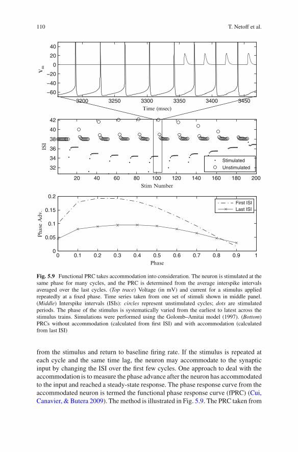
Fig. 5.9 Functional PRC takes accommodation into consideration. The neuron is stimulated at thesame phase for many cycles, and the PRC is determined from the average interspike intervalsaveraged over the last cycles. (Top trace) Voltage (in mV) and current for a stimulus appliedrepeatedly at a fixed phase. Time series taken from one set of stimuli shown in middle panel.(Middle) Interspike intervals (ISIs): circles represent unstimulated cycles; dots are stimulatedperiods. The phase of the stimulus is systematically varied from the earliest to latest across thestimulus trains. Simulations were performed using the Golomb–Amitai model (1997). (Bottom)PRCs without accommodation (calculated from first ISI) and with accommodation (calculatedfrom last ISI)

from the stimulus and return to baseline firing rate. If the stimulus is repeated ateach cycle and the same time lag, the neuron may accommodate to the synapticinput by changing the ISI over the first few cycles. One approach to deal with theaccommodation is to measure the phase advance after the neuron has accommodatedto the input and reached a steady-state response. The phase response curve from theaccommodated neuron is termed the functional phase response curve (fPRC) (Cui,Canavier, & Butera 2009). The method is illustrated in Fig. 5.9. The PRC taken from


the first stimulus interval looks different from the last train. Under conditions wherea neuron may accommodate significantly during network dynamics, the predictionsof network phase locking using the fPRC may produce more accurate results thanpredictions using standard PRCs.

4 Issues in PRC Data Acquisition

On the timescale of a full PRC experiment, the neuron’s firing rate can driftsignificantly. This drift can confound the small phase shifts resulting from thestimuli. “Closed-loop” experimental techniques can be used to counteract this driftand maintain a stable firing rate over the duration of the experiment. In this Sect. 4.1,we introduce the dynamic clamp technique, which enables closed loop experiments(Sect. 4.1), and we describe a method for using the dynamic clamp to control thespike rate in order to reduce firing rate drift over the duration of the experiment(Sect. 4.2). We also show how the dynamic clamp can also be used to choose thephases of stimulation in a quasi-random manner, which can minimize sampling bias(Sect. 4.3).

4.1 Open-loop and Closed-loop Estimation of the PRC

Historically, patch clamp experiments have been done in open loop, where apredetermined stimulus is applied to the neuron and then the neuron’s responseis measured. With the advent of fast analog-to-digital sampling cards in desktopcomputers, it has been possible to design experiments that require real-timeinteractions between the stimulus and the neuron’s dynamics in a closed-loopfashion, called a dynamic-clamp (Sharp, O’Neil, Abbott, & Marder 1993).

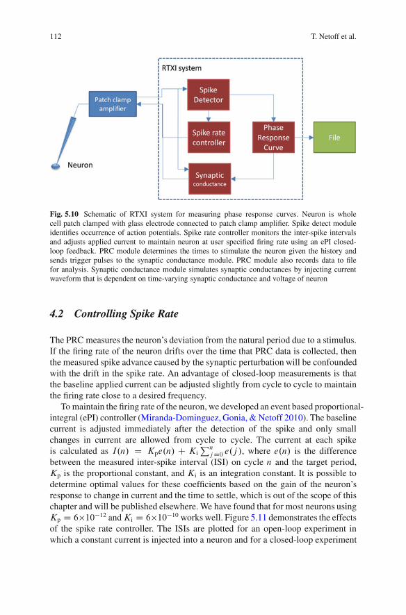
There are many different real-time systems available for dynamic clamp ex-periments (Prinz, Abbott, & Marder 2004). We use the Real-Time eXperimentalInterface (RTXI) system (Dorval, 2nd, Bettencourt, Netoff, & White, 2007; Dorval,Christini, & White, 2001; Dorval, Bettencourt, Netoff, & White, 2008), which isan open-source dynamic clamp based on real-time Linux. It is freely available tothe public for download at http://www.rtxi.org. Modules for controlling the firingrate of the neuron, simulating synapses and measuring the PRC can be downloadedwith the RTXI system. The RTXI system is modular, allowing one to write smallmodules that perform specific tasks and then connect them together to run fullsets of experiments. Figure 5.10 illustrates the modules used to generate PRCsexperimentally. We note that the modular design makes it relatively easy to replacea synaptic conductance module with a module to trigger a picospritzer to injectneurotransmitters proximal to the dendrite to simulate synapses.

http://www.rtxi.org


Fig. 5.10 Schematic of RTXI system for measuring phase response curves. Neuron is wholecell patch clamped with glass electrode connected to patch clamp amplifier. Spike detect moduleidentifies occurrence of action potentials. Spike rate controller monitors the inter-spike intervalsand adjusts applied current to maintain neuron at user specified firing rate using an ePI closed-loop feedback. PRC module determines the times to stimulate the neuron given the history andsends trigger pulses to the synaptic conductance module. PRC module also records data to filefor analysis. Synaptic conductance module simulates synaptic conductances by injecting currentwaveform that is dependent on time-varying synaptic conductance and voltage of neuron

4.2 Controlling Spike Rate

The PRC measures the neuron’s deviation from the natural period due to a stimulus.If the firing rate of the neuron drifts over the time that PRC data is collected, thenthe measured spike advance caused by the synaptic perturbation will be confoundedwith the drift in the spike rate. An advantage of closed-loop measurements is thatthe baseline applied current can be adjusted slightly from cycle to cycle to maintainthe firing rate close to a desired frequency.

To maintain the firing rate of the neuron, we developed an event based proportional-integral (ePI) controller (Miranda-Dominguez, Gonia, & Netoff 2010). The baselinecurrent is adjusted immediately after the detection of the spike and only smallchanges in current are allowed from cycle to cycle. The current at each spikeis calculated as I.n/ D Kpe.n/ C Ki

PnjD0 e.j /, where e.n/ is the difference

between the measured inter-spike interval (ISI) on cycle n and the target period,Kp is the proportional constant, and Ki is an integration constant. It is possible todetermine optimal values for these coefficients based on the gain of the neuron’sresponse to change in current and the time to settle, which is out of the scope of thischapter and will be published elsewhere. We have found that for most neurons usingKp D 6�10�12 andKi D 6�10�10 works well. Figure 5.11 demonstrates the effectsof the spike rate controller. The ISIs are plotted for an open-loop experiment inwhich a constant current is injected into a neuron and for a closed-loop experiment


0 5 10 15 20 25 30 3560

80

100

120

Open loop a b

c d

e f

g h

ISI (

ms)

60

80

100

120

ISI (

ms)

Time (s)

0 5 10 15 20 25 30 35

Time (s)

Closed loop

60 70 80 90 100 110 120 1300

10

20

30 ISI, mean = 92.1317 ms; sdv = 9.9733 ms

Fre

quen

cy

ISI (ms)60 70 80 90 100 110 120 130

ISI (ms)

0

20

40

60ISI, mean = 98.7353 ms; sdv = 7.1793 ms

Fre

quen

cy

0 5 10 15 20 25 30 35

110

120

130

140

150Applied current in open loop

Cur

rent

(pA

)

Time (s)0 5 10 15 20 25 30 35

110

120

130

140

150

Cur

rent

(pA

)

Time (s)

Applied current in closed loop

−10 −5 0 5 10−0.5

0

0.5

1Open loop correlations

Cor

rela

tion

inde

x

j − k−10 −5 0 5 10

−0.5

0

0.5

1

Cor

rela

tion

inde

x

j − k

Closed loop correlations

Fig. 5.11 Spike rate control using ePI controller. (a) In the open-loop configuration, inter-spikeinterval experiences significant drift over the �30 second time interval in which the baselineapplied current is applied, and the average inter-spike interval near the end of the trace (30 to35 s) is over 10 ms away the target interval of 100 ms. Autocorrelations of first lag is nearly zero(see bottom row). This indicates that the error from one cycle is almost completely independentof the previous cycle. (b) With closed-loop control, the inter-spike interval converges quickly tothe target rate of 100 ms. (c and d) The mean inter-spike interval, after the initial transient, isstatistically indistinguishable from the target rate throughout the time interval in which the baselineapplied current is applied. (e and f) During this time, the current injected into the cell is varying tomaintain the neuron close to the target spike rate. Standard deviation of the error in open-loop andclosed-loop are similar, indicating that the closed-loop is only reducing the drift in the inter-spikeinterval rate and not the variability from spike to spike. (g and h) The autocorrelation at the first lagis nearly zero for both the open and closed loop controller. If feedback gain (from the proportionalfeedback coefficient) is too high, the first lag of the autocorrelation will be negative, indicating aringing of the controller


in which a current is adjusted to maintain the neuron at a desired firing rate. Themean ISI in the open-loop experiments undergoes a drift of �10–20 ms, whereas themean ISI in the closed-loop experiments stays very close target period of 100 ms.The autocorrelation is also shown to show that the method does not introduce anysignificant correlation, which occurs if the feedback loop begins to oscillate.

4.3 Phase-Sampling Methods

When generating a PRC for a deterministic computational model of a neuron, it iseasy to systematically sample the response to stimuli at various phases by simplystepping through phases of stimulation, while measuring the phase shift in responseto each stimulus, and restarting the model neuron at a particular initial conditionon the limit cycle after each measurement. In generating PRCs for real neurons,stimuli are delivered sequentially to a oscillating neuron. Experimentally, it is bestto leave several unstimulated interspike intervals after each stimulus to minimizeany interactions between the effects of stimuli. This can be achieved by periodicallystimulating the neuron at intervals several times longer than the neuron’s naturalperiod. Assuming that the neuron has some variability in its period (i.e., jitter) or bychoosing the ratio between the period of the neuron and the period of stimulationcorresponds to an irrational number, this method should sample the period close touniformly and in an unbiased fashion. The advantage of this somewhat haphazardsampling method is that it can be done open loop. The disadvantage is that, inpractice, it may result in oversampling of some phases and undersampling of others.

With a closed-loop experimental system, the phase at which the stimuli areapplied can be selected directly (i.e., by triggering the stimuli off of spike times). Byrandomly selecting the phases of stimulation, you can ensure that there are no biasesintroduced by the experimental protocol. However, even with randomly selectingphases it does not sample the phases most efficiently. Efficiency is paramount inexperiments, because you are racing the slow death of the cell, and thus optimumsampling can improve your PRC estimates. Quasi-random selection of phases, usinga “low-discrepancy” sequence such as a Sobol sequence, can cover the phases in 1p

N

the time as it would take a random sequence, where N is the number of data points(Press 1992). The Sobol sequence as a function of stimulus cycle is illustrated at thebottom of Fig. 5.12.

5 Fitting Functions to PRCs

The interspike intervals measured after applying stimuli can be highly variablefor real neurons, even if the stimuli are applied at the same phase. Because ofthis variability, PRC experiments yield scatter plots of phase shift vs the phase


Fig. 5.12 Sobol sequence to sample the phase of stimulation. With closed-loop experimentsstimuli can be applied at selected phases. The Sobol sequence is a quasi-random sequence, whichefficiently samples phase and minimizes bias. The plot represents the selected stimulus phaseplotted against the stimulus number. The intervals are not random, but not periodic

of stimulation. By appropriately fitting noisy PRC data, a functional relationshipcan be obtained to characterize the mean response of the neuron. This functionalform of the PRC can then be used in conjunction with coupled oscillator theoryto predict of the network behaviors. In this section, we discuss fitting polynomialfunctions (Sect. 5.1) and Fourier series to PRC data (Sect. 5.2) and address the issueof determining optimal number of fit coefficients in terms of the Aikake InformationCriterion (Sect. 5.3). We also discuss statistical models of the variance in PRC data(Sect. 5.4).

5.1 Polynomials

Simple functions that are sufficiently flexible to accommodate the shapes ofPRCs are polynomials (Netoff et al. 2005; Tateno and Robinson 2007). Fittingpolynomials to PRC data is easy to implement: Matlab and many other data analysisprograms have built-in functions that provide the coefficients of a kth degreepolynomial to fit data in the least squares sense. A kth order polynomial fit to PRCdata has the form

PRC.�/ D Ck�k C Ck�1�k�1 C � � � C C2�

2 C C1�CC0;

where PRC(�) is the change in phase as a function of the phase of the stimulus �,Cx’s are the coefficients that are determined by the fit to the data.

Often, spiking neurons are insensitive to perturbations during and immediatelyfollowing spikes. This property is manifested in PRCs with noisy but flat portionsat the early phases, which can sometimes cause spurious oscillations in polynomialfits. These oscillations in the fit can be reduced or eliminated by constraining thePRC to be zero at � D 0 by using the following constrained polynomial:

PRC.�/ D .Ck�k C � � � C C2�

2 C C1� C C0/�


0 0.2 0.4 0.6 0.8 1−0.15

−0.1

−0.05

0

0.05

0.1

0.15

0.2

0.25

Phase

Pha

se A

dvan

ce

Raw Data

6th ord poly

2 Constrained Poly

Fig. 5.13 Free and constrained polynomial fits to PRC data for excitatory input to a neuron. Phaseadvance as a function of stimulus phase is measured for a pyramidal neuron in hippocampus.The neuron was firing at 10 Hz (100 ms intervals). The solid line is an unconstrained 6th orderpolynomial fit (using 7 coefficients) to the points. Notice that the line does not meet the (0,0)point or the (1,0). The dashed line is a two-ended constrained polynomial fit (4 coefficients and 2constraints) that forces the curve to start at (0,0) and end at (1,0)

Moreover, because excitatory inputs can only advance the phase of the next spiketo the point that the neuron actually spikes, excitatory synaptic inputs to spikingneurons generally elicit a PRC with no phase shifts at � D 1. Thus, it is useful toconstrain the fit of the PRC to be zero at both � D 0 and � D 1,

PRC.�/ D .Ck�k C � � � C C2�

2 C C1� C C0/�.1� �/:

To obtain a constrained polynomial for the general period-1 polynomial case, aconstant term C . must added to the above polynomial (Tateno & Robinson 2007).

Examples of a two-end constrained fit and a no-constraint fit to raw PRC datagenerated with excitatory stimuli are illustrated in Fig. 5.13. Figure 5.14 showsexamples of a one-end constrained fit (PRC.�/ D 0), a two-end constrained fitand a no-constraint fit for PRC data generated with inhibitory inputs. In the case ofinhibitory input, there are almost zero phase shifts at early phases, but input causesconsiderable phase shifts at late phases.

5.2 Fourier Series

Due to the periodic nature of many PRCs, PRC data is often fit using Fourierseries (e.g. (Galan, Ermentrout, & Urban 2005; Mancilla, Lewis, Pinto, Rinzel, &Connors 2007; Ota, Nomura, & Aoyagi 2009)). A kth order Fourier series fit to PRCdata can be written as


0 0.2 0.4 0.6 0.8 1−0.5

−0.4

−0.3

−0.2

−0.1

0

0.1

0.2

Phase

Pha

se A

dvan

ce

Raw Data4th ord poly2 Const. Poly1 Const. Poly

Fig. 5.14 Fits to PRC data generated with inhibitory input. PRCs generated with inhibitory inputshave different shapes than those generated with excitatory curves. This is predominantly becausephase shifts are not limited by causality. The largest delays usually occur immediately prior to theneuron spiking. A 4th order polynomial (5 coefficients) fit is plotted with a solid line. A 6th orderpolynomial fit (4 coefficients and 2 constraints) with the beginning constrained to (0,0) and the endto (0,1) is plotted with a dotted line. This function does not fit the right hand side of the data well.A 5th order polynomial fit (4 coefficients and 1 constraint) constrained only at the beginning to(0,0) is plotted with a dot-dashed line. This curve provides the best fit to the data

PRC.�/ D a0 CkX

jD1faj cos.2 j�/C bj sin.2 j�/g;

where the Fourier coefficients are given by

a0 D 1

N

NXnD1

��n; aj D 2

N

NXnD1

��n cos.2 j�n/; bj D 2

N

NXnD1

��n sin.2 j�n/;

where��n is the phase advance measured on stimulus number n that was deliveredat phase �n, andN is the number of data samples. Because many PRCs are zero for� D 0 and � D 1, a better fit for fewer parameters can sometimes be obtained byusing the Fourier sine series

PRC.�/ DkX

jD1bj sin. j�/; bj D 2

N

NXnD1

��n sin. j�n/:


0 0.2 0.4 0.6 0.8 1−0.15

−0.1

−0.05

0

0.05

0.1

0.15

0.2

0.25

Phase

Pha

se A

dvan

ce

1 2 3 4 5 6 7 8 9 10

−1110

−1100

−1090

Number of Coefficients

AIC

Raw Data1 Coef2 Coefs4 Coefs10 Coefs

Optimal number of coefficients

Fig. 5.15 Fourier sine series fit to PRC data for a hippocampal, CA1 pyramidal neuron. (Toppanel) The same raw data as used in Fig. 5.13, but data is fit using a Fourier sine series. Curvesfor fits using different numbers of modes (coefficients) are indicated in the legend. The dotted (1Coef), dot-dashed (2 Coefs) and solid (4 Coefs) show that the fit improves with more coefficients.However, while the dashed line (10 Coefs) technically has lower residual error, the curve exhibitsspurious oscillate, indicating it is overfitting to the data. (Bottom panel) the Akaike InformationCriterion (AIC) is used to determine the optimal number of coefficients. The minimum at 4coefficients indicates that no more than 4 coefficients should be used to fit the PRC

Figure 5.15 illustrates PRC data that is fit using the Fourier sine series withkD 1; 2; 3, and 10. It can be seen that the PRC data set is fit well with only thefirst few modes. Seemingly spurious oscillations appear when the first 10 modes areused to fit the PRC data, suggesting the data are over fit.

One advantage that Fourier series has over polynomials is that one can get areasonably good idea of the shape of the PRC by considering the values of thecoefficients. Furthermore, the H -function, which is defined as H.�i/ D �iC1 ��i � PRC1.�1/C PRC2.1��i/, where PRC1.Œ��i / represents the phase advanceof cell 1 given the synaptic input from cell 2 and PRC2.1��i/ is phase advance ofcell 2 given the approximate phase of cell 1’s input (assuming the phase advanceof cell 1 from cell 2’s input is nearly zero). This is the difference between thetwo neuron’s spikes on can simply be estimated by summing only the odd FourierCoefficients (Galan, Ermentrout, & Urban 2006).


5.3 Over- and Underfitting PRC Data: Akaike InformationCriterion (AIC)

Because Fourier modes are orthogonal to one another, each Fourier coefficient canbe determined sequentially5 and the fitting process can be stopped when the qualityof the fit is satisfactory. As indicated above, when too few modes are included,the data will not be well fit, and as more modes are included, the residual errorof the fit will decrease. However, while including additional modes can decreasethe residual error, the decreased error may not be justified by the additional fittingparameters. To determine how many modes (i.e., number of fitting parameters)should be included, one can use the Akaike information criterion (AIC) (Burnham& Anderson 1998). The Akaike information criterion6 is calculated using thefunction

AIC.k/ D 2k C n

0@ln

0@ 1n

nXjD1

2j .k/21A1A;

where k is the number of fitting parameters (e.g., Fourier coefficients), n is thenumber of points in the data set, and 2j .k/ is the residual error for the j th data pointto the fitted PRC using the k fitting parameters. The optimal number of parametersis determined when AIC(k/ is at its minimum. In Fig. 5.15 (bottom), AIC is plottedas a function of the number of parameters used to fit neuronal PRC data. It can beseen that the minimum occurs at k D 4, thus using more than 4 Fourier modes isoverfitting the PRC data.

The AIC can be used in a similar manner to select the optimal number ofcoefficients for polynomial fits. In fact, the AIC can be used to determine whichmodel (i.e., a Fourier series, a constrained polynomial, etc.) yields the optimal fit.We note, however, that the AIC does not determine whether the fits are statisticallysignificant.

There are alternative approaches to check for validity of fits to PRC data. Galanet al. (2005) fit raw PRC data with a Fourier series and then tested their fit bycomparing it to smoothed data and to fits when the data had been shuffled along thephase axis (abscissa) of the PRC. There are also techniques that employ Bayesianmethods to produce a maximum a posteriori (MAP) estimation of the iPRC ((Ota,Omori, & Aonishi 2009) see also Chap. 8).

5Note that this could be done for polynomial fits too by using orthogonal polynomials (e.g.,Legrendre or Chebychev polynomials).6This formula for the AIC assumes that errors are independently distributed and described by aGaussian distribution.


5.4 Fitting Noise Around the PRC

PRC data for real neurons can be quite noisy. Models that use PRCs to predictphase-locking dynamics usually do not account for the variable phase-responseproperties of neurons. Accounting for the variance of PRC data into these modelscould provide insight into inherently stochastic behaviors such as random leaderswapping and jitter around “stable” phase-locked states. Therefore, it could be veryuseful to obtain a good description of the variability of PRC data.

The variance in PRC data could be generated from several sources. One sourceof variability could be due to external synaptic noise, which will influence theneurons’ spike times along with the simulated input applied through the electrode.We find that blocking synaptic inputs in slice experiments did not dramaticallyreduce the variability (Netoff, unpublished), indicating that synaptic noise may notbe a major source of variability of in vitro PRC data. Another source of variabilitycould be the stochastic fluctuation of the ion channels in the neurons themselves.It has not yet been identified how much of the variability can be attributed to thissource. Identifying the source of the noise may be important in determining how thevariability is related to the shape of the PRC, i.e., the variability in spike time maybe phase dependent.

The variance around the PRC can be strongly phase dependent, as can be seen inFigs. 5.13 and 5.16. For moderate to large-sized inputs, the variability in responseto excitatory inputs earlier in the cycle is usually greater than inputs arriving atthe end of the cycle. There are two causes for the decreased variability at latephases. One is that, as the neuron approaches threshold toward the end of the cycle,synaptic inputs are more likely to directly elicit an action potential. A directlyelicited action potential has significantly less variability than a spike whose timehas been modulated by synaptic inputs early in the cycle. Inhibitory synaptic inputsgenerally do not elicit an action potential, and therefore generate PRCs with moreuniform variability across phase, as shown in Fig. 5.14.

The simplest way to estimate the noise is to bin the data and estimate the standarddeviation in each phase bin. The drawback to this method is that dividing the datainto finer temporal bins results in fewer points in each bin and a less accurateestimate of the standard deviation. This also leads to a piecewise model of thevariance.

Another approach is to fit a continuous function relating the variance to the phase.A simple function that can be fit to the standard deviation around the PRC data forexcitatory stimuli is O�.�/ D n1 C n2

p1 � �. At the end of the cycle when � D 1,

the second term is zero and the standard deviation is equal to n1. As the phase of theinput decreases, the variance increases as a square root of the phase. The motivationfor this function is ad hoc, but is based on the premise that the noise is summedfrom the time of the synaptic input to the end of the period. Therefore, the varianceincreases linearly in time (and the standard deviation as a square root) as the synapticinput is applied earlier in the phase.


Fig. 5.16 Fitting a function to the phase-dependent noise. (Top panel) Raw PRC data fit with afunction to estimate the mean PRC. The standard deviations are shown with error bars at each phaseof the PRC. The slanted blue line represents the line of causality, the maximum phase advancethat can occur (i.e., neuron spikes at time of stimulus). (Bottom panel) The estimated PRC issubtracted from the raw data leaving the residuals of the PRC. The dashed line represents thestandard deviation of the PRC at each phase fit with a simple function using maximum likelihood.The solid line represents a fit function that makes use of the PRCs shape in predicting standarddeviation of the noise

Fitting a function to the noise is not as easy as fitting a function to themean. Rather than optimizing the least squares error from the fit function, wemust find the maximum likelihood function instead. First, we start with removingour best estimate of the PRC from the raw data r.i/ D DATA PRC.�.i// �PRC FIT.�.i// to get the residuals. The residuals of the PRC are plotted in lowerpanel of Fig. 5.16. Next, we need to estimate the probability of seeing the actualmeasured interspike intervals given an estimate of the variance at each phase. We

can choose the initial conditions for the function O�.�/ as: n1 Dq

1n

Pni r.i/

2

and slope N2 D 0. Assuming that the residuals are Gaussianly distributed andindependent, the probability of observing each point given our function for the


variance is p.i/ D 1

ı.i/p2x

exp�� r.i/2

2ı.i/2

�. The total likelihood of all the points

observed is the product of the probabilities at each point, L D Qni p.i/. Because

this probability can become very small very quickly and approach the limits ofthe machine precision, it is usually calculated as the log likelihood, log.L/ D�Pn

i

�12

log.2 O�.i/2/C log.p.i//�. Optimizing the log likelihood by adjusting

the parameters of O� , we can fit the function to the variance of the data. Standarddeviation as a function of phase fitting our function to the noise is shown in Fig. 5.16.

Recently, Ermentrout, Beverlin, 2nd, Troyer, & Netoff (2011) has shown that,when a neuron is subjected to additive white noise, the relationship between thevariance in phase response of a neuron and the shape of the iPRC (Z) is

var.�/ D22�Œ1C ˇZ0.�/�2

Z �

0

Z2.s/ds CZ T

�

Z2.s C ˇZ.�//ds

�;

where 2 is the magnitude of the (white) noise and ˇ is the strength of the(delta function) stimulus. Note that, to leading order in ˇ, this variance is phaseindependent for small ˇ and is equivalent to the intrinsic jitter in the ISIs

var.�/ D22�Z T

0

Z2.s/ds

�:

The parameters 2 and ˇ are usually unknown; therefore, they are used as freeparameters to fit the function to the data optimizing the maximum likelihood. Fits tothe residuals using this function is plotted in Fig. 5.16. This function gives slightlyhigher accuracy in fitting the variance over the simpler square-root function giventhe same number of free parameters.

6 Measuring iPRC with “White Noise” Stimuli

In this section, we outline an alternative method for measuring the infinitesimalphase response curve (iPRC). The method consists of continuously stimulatingthe neuron with a small-amplitude highly fluctuating input over many interspikeintervals, measuring the phase shifts of all spikes due to the stimulus, and thendeconvolving the stimulus and the phase-shifts to obtain the iPRC. The method issuggested in Izhikevich (Izhikevich 2007) and is related to work in Ermentrout et al.(Ermentrout, Galan, & Urban 2007) and Ota et al. (Ota et al. 2009).

As described in Sect. 2.3, we assume that the stimuli are sufficiently small so thatstimulus has a linear effect on the phase of the neuron. Therefore, the phase shift� k of the kth spike during the stimulus is approximated by integral of the productof the iPRCZ.t/ and the stimulus Istim;k.t/ D ��k.t/ over the kth interspike interval

� k D T � Tk ŠZ Tk

0

Z..t//��k.t/dt; (5.12)


where Tk is the duration of the kth interspike interval, T is the intrinsic period of theneuron, and .t/ is the absolute phase of the neuron. The stimulus ��k.t/ is chosento be a piecewise constant function that is a realization of Gaussian white noise,i.e., time is broken up into very small intervals of width �t and the amplitudes of��k.t/ is each subinterval is drawn from a Gaussian distribution with zero mean andvariance �2, where � is assumed to be small. Note that this stimulus is composed ofa wide range of Fourier modes that will typically form a basis for the iPRC Z.

The phase of the unstimulated neuron increases linearly with time, and thereforewe approximate the phase of the weakly stimulated neuron as .t/ D T=Tkt . Bychanging variables so that the integration is in terms of phase, (5.12) becomes

� k ŠZ T

D0Z./��k.t.//

Tk

Td: (5.13)

Note that, in this form, the upper limit of integration is independent of k, i.e., itis the same for all cycles. By discretizing phase into M � 20 equal bins of width� D T=M , (5.13) can be approximated using a middle Riemann sum

� k ŠMXjD1

Z.j /h��k.tj /iTkT�; (5.14)

where h��k.tj /i is the average of the stimulus in the j th bin during the kth cycle

h��k.tj /i 1�

Z tjC�k=2

tj��k=2��k.t/dt :

and j D �j � 1

2

� , tj D Tk

Tj , and�k D Tk

T� . Figure 5.17 shows an example

of a fluctuating stimuli (second panel) and its binned and averaged version for asingle cycle andM D 20.

If the stimulus is presented over N cycles, (5.14) with k D 1: : :N yields asystem of N equations with M unknowns, i.e., the equally spaced points on theiPRC Z.j /. In matrix notation, this system of equations is

� Š NZ (5.15)

where � is an N � 1 vector containing the phase shifts of each spike duringthe stimulus, is an N � M matrix in which the j ,k element is h��k.tj /i TkT �containing the binned and averaged stimuli for each spike, and NZ is a M �1 vector containing the points on the iPRC. Thus, estimation of the iPRC isreduced to solving a “simple” linear algebra problem. Typically, there should bemore phase shifts recorded (N/ than points on the iPRC (M/, so that system(5.15) is overdetermined and can be solved using a least squares approximation.Figure 5.18 shows an example of an iPRC estimated using this technique for the


Fig. 5.17 [Top panel] The membrane potential of a Hodgkin–Huxley model neuron subject toan applied current of 10�A=cm2 for a single cycle. The blue trace represents the unperturbedoscillation, and the red trace represents the oscillation perturbed by the “white noise” stimulus inthe middle panel. [Middle panel] A realization of the “white noise” stimuli ��k.t/ that is (sampledwith a time step �t D 0:005ms and � D 1:5�A=cm2/. [Third panel] The stimulus in the secondpanel after being divided into M D 20 bins and averaged for each bin. The amplitudes from thisaveraged signal make up one row of the matrix

Hodgkin–Huxley (HH) model neuron with additive current noise. There are 20points on the estimated iPRC (M D 20) and 40 spikes were sampled (N D 40). Theerror in this estimated iPRC is 0.30, where the error is computed as the normalized`2-norm

NZ �Za

2

ıZa

2, where Za is the iPRC calculated using the adjoint

method evaluated at the appropriate phases.Because � is a random matrix, it could sometimes have a high condition number,

which could lead to significant error in the estimation of the discretized iPRC NZ.However, we can reduce the chance of this error by making the number of spikesconsidered N sufficiently larger than the number of points on the estimated iPRCM . Figure 5.19 shows the decrease in the error of the estimation of the iPRC forthe HH model neuron as the number of spikes is increased. Note the steep initialdecrease in the error. In practice, we find that about twice as many spikes (phaseshifts) as number of points on the estimated iPRC yields a relatively low error.Typically, 20 points provides a good representation of an iPRC for a spiking neuron.


0 2 4 6 8 10 12 14−0.3

−0.2

−0.1

0

0.1

0.2

0.3

0.4

0.5

0.6

Phase (msec)

iPRC from Adjoint MethodiPRC from "White Noise" Estimation

Fig. 5.18 Example of an estimated iPRC using the “white noise” method for the Hodgkin–Huxleyneuron with “unknown” additive noise. The red trace is the iPRC calculated using the adjointmethod (Ermentrout & Kopell 1991) and the crosses are the estimates of the iPRC found fromsolving (5.15) for Z. There are M D 20 points on the estimated iPRC, and N D 40 cycles wereused to calculate the iPRC. The stimulus has parameters �t D 0:005ms and � D 1:5�A=cm2.The signal (stimulus) to noise ratio was �5.0. The error in the estimated iPRC is 0.30

a b

Fig. 5.19 Error in the estimated iPRC withM D 20 versus the number of interspike intervals. Theerror in the estimated iPRC is computed as

NZ �Za

2=Za

2, where Za is the iPRC calculated

using the adjoint method evaluated at the appropriate phases. (a) The system with no noise. (b)The system with “unknown” additive white noise with signal (stimulus) to noise ratio of �5.0.Estimates were made for M D 20 points on the iPRCs. For both cases, the error decreases quicklyas more trials are recorded. The stimulus has parameters �t D 0:005ms and � D 1:5�A=cm2 in(a) and � D 8�A=cm2 in (b). 700 trials were used to generate the statistics for every point on thegraphs. Data points are mean values and error bars represent the limits that included ˙30% of data


a b

Fig. 5.20 Error in the estimated iPRC versus signal strength. The error is calculated as describedin Fig. 5.19. The error is shown as a function of the strength of the random signal when (a) thesystem has no noise and (b) the system has “unknown” additive white noise. In both cases, there isan optimal value of the signal strength which minimizes the error in the estimation. Furthermore,both the mean and standard deviation of the error increase significantly as the signal strengthbecomes too large, i.e., the neuron no longer responds linearly. Estimates were made withN D 40

recorded spikes, M D 20 points on the iPRCs, and �t D 0:005ms. The unknown noise had amagnitude such that the signal (stimulus) to noise ratio was �5.0 when � D 8�A=cm2. 700 trialswere used to generate the statistics for every point on the graphs. Data points are mean values anderror bars represent the limits that included ˙30% of data

Therefore, if a neuron is firing at 10–20 Hz on average, and the phase shifts aremeasured over 40 spikes, it only takes 2–4 seconds to record the data needed toestimate the iPRC.

The strength of the random stimulus, � , also affects the quality of the estimatediPRC. In practice, the stimulus amplitude must be small in order for the estimationto be theoretically valid, but it must also be large enough to overcome the intrinsicnoise in the system. Figure 5.20 plots the error in the estimation as a function of� when there is no unknown additive noise in the system (a), and when there isunknown additive noise in the system (b). In both cases, there is an optimal value of� that minimizes the error in our estimation. This optimal value is larger when thereis noise in the system.

While the method described above is perhaps the most straightforward “whitenoise” method, other methods that use white noise stimuli to measure the iPRChave also been proposed. Ermentrout et al. 2007 showed that, when an oscillatingneuron is stimulated with small amplitude white noise, the spike triggered average(STA) is proportional to the derivative of its iPRC. As such, the iPRC can becalculated by integrating the STA. Ota (Ota et al. 2009) recently addressed severalpractical issues concerning the results of Ermentrout (Ermentrout et al. 2007) andoutlined a procedure to estimate iPRCs for real neurons by using an appropriatelyweighted STA.


Izhikevich (Izhikevich 2007) comments that white noise methods for iPRCestimation should be more immune to noise than standard pulse methods becausethe stimulus fluctuations are spread over the entire cycle and not concentrated atthe moments of pulses. However, to our knowledge, there has been no systematiccomparison of the white noise methods and the standard pulse method. More workis needed to determine the optimal method for different situations (i.e., differentnoise levels, limitations on number of spikes, etc.). Furthermore, we expect thatrefinements could be made to improve most of these methods.

7 Summary

• The first step in generating a phase response curve for a neuron is choosingan appropriate stimulus waveform. When estimating the infinitesimal PRC (foruse with theory of weakly coupled oscillators), a small brief delta-function-likestimulus pulse can be used. If synaptic inputs are not expected to sum linearly,then a realistic synaptic waveform should be used to measure the PRC to includethe proper nonlinear responses of the neuron.

• The effects of a pulse stimulus on neuronal firing may last longer than a singlecycle and give rise to measureable changes in ISIs in the cycles following thestimulated interval. These effects can be quantified with secondary and higherorder PRCs and can be incorporated into models to increase their accuracy(Maran & Canavier 2008; Oprisan & Canavier 2001). Alternatively, the stimuluscan be repeated at the same phase until the higher order effects accumulate andstabilize, and then the steady state response to the synaptic input at a phase canbe measured. This results in measuring a “functional PRC” (Cui et al. 2009).

• Neurons exhibit considerable amounts of noise, making phase response datavariable. There are two sources of noise: drift and jitter. Drift in the dynamics ofthe neuron occurs from slow timescale neuronal processes and “run down” (slowdeath) of the neuron during the experiment. This can be compensated to somedegree by maintaining the firing rate of the neuron with a spike rate controller.While it is not a panacea, it keeps one aspect (the period) approximately constantover the duration of the experiment.

• To decrease the duration of the PRC experiment and thereby reduce the effects ofdrift on PRC estimation, the sampling of stimulus phase can be optimized. Usinga Sobol sequence to sample the phases is much more efficient than random, orquasi-periodic sampling.

• The jitter in the phase response can be overcome by fitting a function to thedata to estimate the deterministic portion of the neuron’s PRC. Polynomialswith constraints or Fourier series usually provide good fits to PRC data. TheAkaike information criterion can be used to determine the appropriate number ofcoefficients when fitting either a polynomial or the Fourier series.

• The variability in a neuron’s phase response can also be quantified and modeled.Ermentrout, Beverlin, 2nd, Troyer, & Netoff (2011) has recently shown that the


phase dependence of the variance is dependent on the shape of the PRC. Wealso present a simple function that can be fit to the variance by optimizing themaximum likelihood that does a reasonably good job.

• White noise stimulus approaches provide alternatives to pulse stimulation meth-ods for measuring infinitesimal PRCs. This approach uses linear algebra toestimate the iPRC from neuronal response to white noise applied to several pe-riods. More work must be done to optimize these methods and to systematicallycompare them to the standard pulse stimulation methods.

Acknowledgments TJL and MAS were supported by the National Science Foundation undergrants DMS-09211039 (TJL), DMS-0518022 (TJL), TIN was supported by NSF CAREER AwardCBET-0954797 (TIN).

References

Burnham, K. P., & Anderson, D. R. (1998). Model selection and inference: A practical information-theoretic approach. New York: Springer.

Canavier, C. C. (2005). The application of phase resetting curves to the analysis of patterngenerating circuits containing bursting neurons. In S. Coombes, P. C. Bressloff & N. J.Hackensack (Eds.), Bursting: The genesis of rhythm in the nervous system (pp. 175–200) WorldScientific.

Cruikshank, S. J., Lewis, T. J., & Connors, B. W. (2007). Synaptic basis for intense thalamocorticalactivation of feedforward inhibitory cells in neocortex. Nature Neuroscience, 10(4), 462–468.doi:10.1038/nn1861.

Cui, J., Canavier, C. C., & Butera, R. J. (2009). Functional phase response curves: A methodfor understanding synchronization of adapting neurons. Journal of Neurophysiology, 102(1),387–398. doi:10.1152/jn.00037.2009.

Dorval, A. D., 2nd, Bettencourt, J., Netoff, T. I., & White, J. A. (2007). Hybrid neuronal networkstudies under dynamic clamp. Methods in Molecular Biology (Clifton, N.J.), 403, 219–231.doi:10.1007/978–1–59745–529–9 15.

Dorval, A. D., Bettencourt, J. C., Netoff, T. I., & White, J. A. (2008). Hybrid neuronal networkstudies under dynamic clamp. In Applied patch clamp Humana.

Dorval, A. D., Christini, D. J., & White, J. A. (2001). Real-time linux dynamic clamp: A fast andflexible way to construct virtual ion channels in living cells. Ann Biomed Eng, 29(10), 897–907.

Ermentrout, G. B., Beverlin, B., 2nd, Troyer, T., & Netoff, T. I. (2011). The variance of phase-resetting curves. J Comput Neurosci, [Epub ahead of print].

Ermentrout, G. B., & Chow, C. C. (2002). Modeling neural oscillations. Physiol Behav, 77(4–5),629–633.

Ermentrout, G. B., Galan, R. F., & Urban, N. N. (2007). Relating neural dynamics to neural coding.Physical Review Letters, 99(24), 248103.

Ermentrout, G. B., & Kopell, N. (1991). Multiple pulse interactions and averaging in systems ofcoupled neural oscillators. J Math Biol, 29, 195–217.

Galan, R. F., Ermentrout, G. B., & Urban, N. N. (2005). Efficient estimation of phase-resettingcurves in real neurons and its significance for neural-network modeling. Physical ReviewLetters, 94(15), 158101.

Galan, R. F., Bard Ermentrout, G., & Urban, N. N. (2006). Predicting synchronized neuralassemblies from experimentally estimated phase-resetting curves. Neurocomputing, 69(10–12),1112–1115. doi:DOI: 10.1016/j.neucom.2005.12.055.


Golomb, D., & Amitai, Y. (1997). Propagating neuronal discharges in neocortical slices: Compu-tational and experimental study. Journal of Neurophysiology, 78(3), 1199–1211.

Hille, B. (1992). Ionic channels of excitable membranes (2nd ed.). Sunderland: Sinauer Associates.Izhikevich, E. M. (2007). Dynamical systems in neuroscience: The geometry of excitability and

bursting. Cambridge: MIT.Kuramoto, Y. (1984). Chemical oscillations, waves, and turbulence. Berlin: Springer.Lewis, T. J., & Rinzel, J. (2003). Dynamics of spiking neurons connected by both inhibitory and

electrical coupling. Journal of Computational Neuroscience, 14(3), 283–309.Mancilla, J. G., Lewis, T. J., Pinto, D. J., Rinzel, J., & Connors, B. W. (2007). Synchro-

nization of electrically coupled pairs of inhibitory interneurons in neocortex. The Journalof Neuroscience: The Official Journal of the Society for Neuroscience, 27(8), 2058–2073.doi:10.1523/JNEUROSCI.2715–06.2007.

Maran, S. K., & Canavier, C. C. (2008). Using phase resetting to predict 1:1 and 2:2 locking intwo neuron networks in which firing order is not always preserved. Journal of ComputationalNeuroscience, 24(1), 37–55. doi:10.1007/s10827–007–0040-z.

Miranda-Dominguez, O., Gonia, J., & Netoff, T. I. (2010). Firing rate control of a neuronusing a linear proportional-integral controller. Journal of Neural Engineering, 7(6), 066004.doi:10.1088/1741–2560/7/6/066004.

Netoff, T. I., Acker, C. D., Bettencourt, J. C., & White, J. A. (2005). Beyond two-cell networks:Experimental measurement of neuronal responses to multiple synaptic inputs. Journal ofComputational Neuroscience, 18(3), 287–295. doi:10.1007/s10827–005–0336–9.

Netoff, T. I., Banks, M. I., Dorval, A. D., Acker, C. D., Haas, J. S., Kopell, N., & White, J. A.(2005). Synchronization in hybrid neuronal networks of the hippocampal formation. Journal ofNeurophysiology, 93(3), 1197–1208. doi:00982.2004 [pii]; 10.1152/jn.00982.2004.

Oprisan, S. A., & Canavier, C. C. (2001). Stability analysis of rings of pulse-coupled oscillators:The effect of phase-resetting in the second cycle after the pulse is important at synchrony andfor long pulses. Differential Equations and Dynamical Systems, 9, 243–258.

Ota, K., Omori, T., & Aonishi, T. (2009). MAP estimation algorithm for phase response curvesbased on analysis of the observation process. Journal of Computational Neuroscience, 26(2),185–202. doi:10.1007/s10827–008–0104–8.

Ota, K., Nomura, M., & Aoyagi, T. (2009). Weighted spike-triggered average of a fluctuat-ing stimulus yielding the phase response curve. Physical Review Letters, 103(2), 024101.doi:10.1103/PhysRevLett.103.024101.

Press, W. H. (1992). Numerical recipes in C: The art of scientific computing (2nd ed.). Cambridge:Cambridge University Press.

Prinz, A. A., Abbott, L. F., & Marder, E. (2004). The dynamic clamp comes of age. Trends inNeurosciences, 27(4), 218–224. doi:10.1016/j.tins.2004.02.004.

Sharp, A. A., O’Neil, M. B., Abbott, L. F., & Marder, E. (1993). Dynamic clamp: Computer-generated conductances in real neurons. J Neurophysiol, 69(3), 992–995.

Tateno, T., & Robinson, H. P. (2007). Phase resetting curves and oscillatory stabil-ity in interneurons of rat somatosensory cortex. Biophysical Journal, 92(2), 683–695.doi:10.1529/biophysj.106.088021.

Van Vreeswijk, C., Abbott, L. F., & Ermentrout, G. B. (1994). When inhibition not excitationsynchronizes neural firing. J Comput Neurosci, 1(4), 313–321.

Date post:	27-Feb-2018
Category:	Documents
Upload:	lamngoc
View:	218 times
Download:	2 times

Chapter 5 Experimentally Estimating Phase Response Curves...

Documents