Chapter 5 Prediction Prerequisites • The best linear predictor. • Some idea of what a basis of a vector space is. Objectives • Understand that prediction using a long past can be difficult because a large matrix has to be inverted, thus alternative, recursive method are often used to avoid direct inversion. • Understand the derivation of the Levinson-Durbin algorithm, and why the coefficient, φ t,t , corresponds to the partial correlation between X 1 and X t+1 . • Understand how these predictive schemes can be used write space of sp(X t ,X t-1 ,...,X 1 ) in terms of an orthogonal basis sp(X t - P X t-1 ,X t-2 ,...,X 1 (X t ),...,X 1 ). • Understand how the above leads to the Wold decomposition of a second order stationary time series. • To understand how to approximate the prediction for an ARMA time series into a scheme which explicitly uses the ARMA structure. And this approximation improves geometrically, when the past is large. One motivation behind fitting models to a time series is to forecast future unobserved observa- tions - which would not be possible without a model. In this chapter we consider forecasting, based on the assumption that the model and/or autocovariance structure is known. 133
Transcript
Chapter 5
Prediction
Prerequisites
• The best linear predictor.
• Some idea of what a basis of a vector space is.
Objectives
• Understand that prediction using a long past can be di�cult because a large matrix has to
be inverted, thus alternative, recursive method are often used to avoid direct inversion.
• Understand the derivation of the Levinson-Durbin algorithm, and why the coe�cient, �t,t,
corresponds to the partial correlation between X1
and Xt+1
.
• Understand how these predictive schemes can be used write space of sp(Xt, Xt�1
, . . . , X1
) in
terms of an orthogonal basis sp(Xt � PXt�1
,Xt�2
,...,X1
(Xt), . . . , X1
).
• Understand how the above leads to the Wold decomposition of a second order stationary
time series.
• To understand how to approximate the prediction for an ARMA time series into a scheme
which explicitly uses the ARMA structure. And this approximation improves geometrically,
when the past is large.
One motivation behind fitting models to a time series is to forecast future unobserved observa-
tions - which would not be possible without a model. In this chapter we consider forecasting, based
on the assumption that the model and/or autocovariance structure is known.
133
5.1 Forecasting given the present and infinite past
In this section we will assume that the linear time series {Xt} is both causal and invertible, that is
Xt =1X
j=0
aj"t�j =1X
i=1
biXt�i + "t, (5.1)
where {"t} are iid random variables (recall Definition 2.2.2). Both these representations play an
important role in prediction. Furthermore, in order to predict Xt+k given Xt, Xt�1
, . . . we will
assume that the infinite past is observed. In later sections we consider the more realistic situation
that only the finite past is observed. We note that since Xt, Xt�1
, Xt�2
, . . . is observed that we can
obtain "⌧ (for ⌧ t) by using the invertibility condition
"⌧ = X⌧ �1X
i=1
biX⌧�i.
Now we consider the prediction of Xt+k given {X⌧ ; ⌧ t}. Using the MA(1) presentation
(since the time series is causal) of Xt+k we have
Xt+k =1X
j=0
aj+k"t�j
| {z }
innovations are ‘observed’
+k�1
X
j=0
aj"t+k�j
| {z }
future innovations impossible to predict
,
since E[Pk�1
j=0
aj"t+k�j |Xt, Xt�1
, . . .] = E[Pk�1
j=0
aj"t+k�j ] = 0. Therefore, the best linear predictor
of Xt+k given Xt, Xt�1
, . . ., which we denote as Xt(k) is
Xt(k) =1X
j=0
aj+k"t�j =1X
j=0
aj+k(Xt�j �1X
i=1
biXt�i�j). (5.2)
Xt(k) is called the k-step ahead predictor and it is straightforward to see that it’s mean squared
error is
E [Xt+k �Xt(k)]2 = E
2
4
k�1
X
j=0
aj"t+k�j
3
5
2
= var["t]kX
j=0
a2j , (5.3)
where the last line is due to the uncorrelatedness and zero mean of the innovations.
Often we would like to obtain the k-step ahead predictor for k = 1, . . . , n where n is some
134
time in the future. We now explain how Xt(k) can be evaluated recursively using the invertibility
assumption.
Step 1 Use invertibility in (5.1) to give
Xt(1) =1X
i=1
biXt+1�i,
and E [Xt+1
�Xt(1)]2 = var["t]
Step 2 To obtain the 2-step ahead predictor we note that
Xt+2
=1X
i=2
biXt+2�i + b1
Xt+1
+ "t+2
=1X
i=2
biXt+2�i + b1
[Xt(1) + "t+1
] + "t+2
,
thus it is clear that
Xt(2) =1X
i=2
biXt+2�i + b1
Xt(1)
and E [Xt+2
�Xt(2)]2 = var["t]
�
b21
+ 1�
= var["t]�
a22
+ a21
�
.
Step 3 To obtain the 3-step ahead predictor we note that
Xt+3
=1X
i=3
biXt+2�i + b2
Xt+1
+ b1
Xt+2
+ "t+3
=1X
i=3
biXt+2�i + b2
(Xt(1) + "t+1
) + b1
(Xt(2) + b1
"t+1
+ "t+2
) + "t+3
.
Thus
Xt(3) =1X
i=3
biXt+2�i + b2
Xt(1) + b1
Xt(2)
and E [Xt+3
�Xt(3)]2 = var["t]
⇥
(b2
+ b21
)2 + b21
+ 1⇤
= var["t]�
a23
+ a22
+ a21
�
.
135
Step k Using the arguments above it is easily seen that
Xt(k) =1X
i=k
biXt+k�i +k�1
X
i=1
biXt(k � i).
Thus the k-step ahead predictor can be recursively estimated.
We note that the predictor given above it based on the assumption that the infinite past is
observed. In practice this is not a realistic assumption. However, in the special case that time
series is an autoregressive process of order p (with AR parameters {�j}pj=1
) and Xt, . . . , Xt�m is
observed where m � p� 1, then the above scheme can be used for forecasting. More precisely,
Xt(1) =pX
j=1
�jXt+1�j
Xt(k) =pX
j=k
�jXt+k�j +k�1
X
j=1
�jXt(k � j) for 2 k p
Xt(k) =pX
j=1
�jXt(k � j) for k > p. (5.4)
However, in the general case more sophisticated algorithms are required when only the finite
past is known.
Example: Forecasting yearly temperatures
We now fit an autoregressive model to the yearly temperatures from 1880-2008 and use this model
to forecast the temperatures from 2009-2013. In Figure 5.1 we give a plot of the temperature time
series together with it’s ACF. It is clear there is some trend in the temperature data, therefore we
have taken second di↵erences, a plot of the second di↵erence and its ACF is given in Figure 5.2.
We now use the command ar.yule(res1,order.max=10) (we will discuss in Chapter 7 how this
function estimates the AR parameters) to estimate the the AR parameters. The function ar.yule
uses the AIC to select the order of the AR model. When fitting the second di↵erences from (from
1880-2008 - a data set of length of 127) the AIC chooses the AR(7) model
Xt = �1.1472Xt�1
� 1.1565Xt�2
� 1.0784Xt�3
� 0.7745Xt�4
� 0.6132Xt�5
� 0.3515Xt�6
� 0.1575Xt�7
+ "t,
136
Time
temp
1880 1900 1920 1940 1960 1980 2000
−0.5
0.0
0.5
0 5 10 15 20 25 30
−0.2
0.0
0.2
0.4
0.6
0.8
1.0
Lag
ACF
Series global.mean
Figure 5.1: Yearly temperature from 1880-2013 and the ACF.
Time
second.differences
1880 1900 1920 1940 1960 1980 2000
−0.6
−0.4
−0.2
0.0
0.2
0.4
0.6
0 5 10 15 20 25 30
−0.5
0.0
0.5
1.0
Lag
ACF
Series diff2
Figure 5.2: Second di↵erences of yearly temperature from 1880-2013 and its ACF.
with var["t] = �2 = 0.02294. An ACF plot after fitting this model and then estimating the residuals
{"t} is given in Figure 5.3. We observe that the ACF of the residuals ‘appears’ to be uncorrelated,
which suggests that the AR(7) model fitted the data well. Later we cover the Ljung-Box test, which
is a method for checking this claim. However since the residuals are estimated residuals and not
the true residual, the results of this test need to be taken with a large pinch of salt. We will show
that when the residuals are estimated from the data the error bars given in the ACF plot are not
correct and the Ljung-Box test is not pivotal (as is assumed when deriving the limiting distribution
137
under the null the model is correct). By using the sequence of equations
0 5 10 15 20
−0.2
0.00.2
0.40.6
0.81.0
Lag
ACF
Series residuals
Figure 5.3: An ACF plot of the estimated residuals {b"t}.
X127
(1) = �1.1472X127
� 1.1565X126
� 1.0784X125
� 0.7745X124
� 0.6132X123
�0.3515X122
� 0.1575X121
X127
(2) = �1.1472X127
(1)� 1.1565X127
� 1.0784X126
� 0.7745X125
� 0.6132X124
�0.3515X123
� 0.1575X122
X127
(3) = �1.1472X127
(2)� 1.1565X127
(1)� 1.0784X127
� 0.7745X126
� 0.6132X125
�0.3515X124
� 0.1575X123
X127
(4) = �1.1472X127
(3)� 1.1565X127
(2)� 1.0784X127
(1)� 0.7745X127
� 0.6132X126
�0.3515X125
� 0.1575X124
X127
(5) = �1.1472X127
(4)� 1.1565X127
(3)� 1.0784X127
(2)� 0.7745X127
(1)� 0.6132X127
�0.3515X126
� 0.1575X125
.
We can use X127
(1), . . . , X127
(5) as forecasts of X128
, . . . , X132
(we recall are the second di↵erences),
which we then use to construct forecasts of the temperatures. A plot of the second di↵erence
forecasts together with the true values are given in Figure 5.4. From the forecasts of the second
di↵erences we can obtain forecasts of the original data. Let Yt denote the temperature at time t
138
and Xt its second di↵erence. Then Yt = �Yt�2
+ 2Yt�1
+Xt. Using this we have
bY127
(1) = �Y126
+ 2Y127
+X127
(1)
bY127
(2) = �Y127
+ 2Y127
(1) +X127
(2)
bY127
(3) = �Y127
(1) + 2Y127
(2) +X127
(3)
and so forth.
We note that (5.3) can be used to give the mse error. For example
E[X128
� X127
(1)]2 = �2t
E[X128
� X127
(1)]2 = (1 + �21
)�2t
If we believe the residuals are Gaussian we can use the mean squared error to construct confidence
intervals for the predictions. Assuming for now that the parameter estimates are the true param-
eters (this is not the case), and Xt =P1
j=0
j(b�)"t�j is the MA(1) representation of the AR(7)
model, the mean square error for the kth ahead predictor is
�2k�1
X
j=0
j(b�)2 (using (5.3))
thus the 95% CI for the prediction is
2
4Xt(k)± 1.96�2k�1
X
j=0
j(b�)2
3
5 ,
however this confidence interval for not take into account Xt(k) uses only parameter estimators
and not the true values. In reality we need to take into account the approximation error here too.
If the residuals are not Gaussian, the above interval is not a 95% confidence interval for the
prediction. One way to account for the non-Gaussianity is to use bootstrap. Specifically, we rewrite
the AR(7) process as an MA(1) process
Xt =1X
j=0
j(b�)"t�j .
139
Hence the best linear predictor can be rewritten as
Xt(k) =1X
j=k
j(b�)"t+k�j
thus giving the prediction error
Xt+k �Xt(k) =k�1
X
j=0
j(b�)"t+k�j .
We have the prediction estimates, therefore all we need is to obtain the distribution ofPk�1
j=0
j(b�)"t+k�j .
This can be done by estimating the residuals and then using bootstrap1 to estimate the distribu-
tion ofPk�1
j=0
j(b�)"t+k�j , using the empirical distribution ofPk�1
j=0
j(b�)"⇤t+k�j . From this we can
construct the 95% CI for the forecasts.
2000 2002 2004 2006 2008 2010 2012
−0.3
−0.2
−0.1
0.00.1
0.20.3
year
second
differe
nce
●
●
●
●
●
●
●
●
●
●
●
●
●
●
= forecast
● = true value
Figure 5.4: Forecasts of second di↵erences.
A small criticism of our approach is that we have fitted a rather large AR(7) model to time
1Residual bootstrap is based on sampling from the empirical distribution of the residuals i.e. constructthe “bootstrap” sequence {"⇤t+k�j}j by sampling from the empirical distribution bF (x) = 1
n
Pnt=p+1 I(b"t
x) (where b"t = Xt � Ppj=1
b�jXt�j). This sequence is used to construct the bootstrap estimatorPk�1
j=0 j(b�)"⇤t+k�j . By doing this several thousand times we can evaluate the empirical distribution ofPk�1
j=0 j(b�)"⇤t+k�j using these bootstrap samples. This is an estimator of the distribution function ofPk�1
j=0 j(b�)"t+k�j .
140
series of length of 127. It may be more appropriate to fit an ARMA model to this time series.
Exercise 5.1 In this exercise we analyze the Sunspot data found on the course website. In the data
analysis below only use the data from 1700 - 2003 (the remaining data we will use for prediction).
In this section you will need to use the function ar.yw in R.
(i) Fit the following models to the data and study the residuals (using the ACF). Using this
decide which model
Xt = µ+A cos(!t) +B sin(!t) + "t|{z}
AR
or
Xt = µ+ "t|{z}
AR
is more appropriate (take into account the number of parameters estimated overall).
(ii) Use these models to forecast the sunspot numbers from 2004-2013.
In next few sections we will consider prediction/forecasting for stationary time series. In particular
to find the best linear predictor of Xt+1
given the finite past Xt, . . . , X1
. Setting up notation our
aim is to find
Xt+1|t = PX1
,...,Xt
(Xt+1
) = Xt+1|t,...,1 =tX
j=1
�t,jXt+1�j ,
where {�t,j} are chosen to minimise the mean squared error min�t
E(Xt+1
�Ptj=1
�t,jXt+1�j)2.
Basic results from multiple regression show that
0
B
B
B
@
�t,1...
�t,t
1
C
C
C
A
= ⌃�1
t rt,
where (⌃t)i,j = E(XiXj) and (rt)i = E(Xt�iXt+1
). Given the covariances this can easily be done.
However, if t is large a brute force method would require O(t3) computing operations to calculate
(5.7). Our aim is to exploit stationarity to reduce the number of operations. To do this, we will
briefly discuss the notion of projections on a space, which help in our derivation of computationally
more e�cient methods.
Before we continue we first discuss briefly the idea of a a vector space, inner product spaces,
Hilbert spaces, spans and basis. A more complete review is given in Brockwell and Davis (1998),
Chapter 2.
First a brief definition of a vector space. X is called an vector space if for every x, y 2 X and
a, b 2 R (this can be generalised to C), then ax + by 2 X . An inner product space is a vector
space which comes with an inner product, in other words for every element x, y 2 X we can defined
an innerproduct hx, yi, where h·, ·i satisfies all the conditions of an inner product. Thus for every
element x 2 X we can define its norm as kxk = hx, xi. If the inner product space is complete
(meaning the limit of every sequence in the space is also in the space) then the innerproduct space
is a Hilbert space (see wiki).
Example 5.2.1 (i) The classical example of a Hilbert space is the Euclidean space Rn where
the innerproduct between two elements is simply the scalar product, hx,yi =Pni=1
xiyi.
142
(ii) The subset of the probability space (⌦,F , P ), where all the random variables defined on ⌦
have a finite second moment, ie. E(X2) =R
⌦
X(!)2dP (!) < 1. This space is denoted as
L2(⌦,F , P ). In this case, the inner product is hX,Y i = E(XY ).
(iii) The function space L2[R, µ], where f 2 L2[R, µ] if f is mu-measureable and
Z
R|f(x)|2dµ(x) < 1,
is a Hilbert space. For this space, the inner product is defined as
hf, gi =Z
Rf(x)g(x)dµ(x).
In this chapter we will not use this function space, but it will be used in Chapter ?? (when
we prove the Spectral representation theorem).
It is straightforward to generalize the above to complex random variables and functions defined
on C. We simply need to remember to take conjugates when defining the innerproduct, ie. hX,Y i =E(XY ) and hf, gi = RC f(z)g(z)dµ(z).
In this chapter our focus will be on certain spaces of random variables which have a finite variance.
Basis
The random variables {Xt, Xt�1
, . . . , X1
} span the space X 1
t (denoted as sp(Xt, Xt�1
, . . . , X1
)), if
for every Y 2 X 1
t , there exists coe�cients {aj 2 R} such that
Y =tX
j=1
ajXt+1�j . (5.5)
Moreover, sp(Xt, Xt�1
, . . . , X1
) = X 1
t if for every {aj 2 R}, Ptj=1
ajXt+1�j 2 X 1
t . We now
define the basis of a vector space, which is closely related to the span. The random variables
{Xt, . . . , X1
} form a basis of the space X 1
t , if for every Y 2 X 1
t we have a representation (5.5) and
this representation is unique. More precisely, there does not exist another set of coe�cients {bj}such that Y =
Ptj=1
bjXt+1�j . For this reason, one can consider a basis as the minimal span, that
is the smallest set of elements which can span a space.
Definition 5.2.1 (Projections) The projection of the random variable Y onto the space spanned
143
by sp(Xt, Xt�1
, . . . , X1
) (often denoted as PXt
,Xt�1
,...,X1
(Y)) is defined as PXt
,Xt�1
,...,X1
(Y) =Pt
j=1
cjXt+1�j,
where {cj} is chosen such that the di↵erence Y �P(X
t
,Xt�1
,...,X1
)
(Yt) is uncorrelated (orthogonal/per-
pendicular) to any element in sp(Xt, Xt�1
, . . . , X1
). In other words, PXt
,Xt�1
,...,X1
(Yt) is the best
linear predictor of Y given Xt, . . . , X1
.
Orthogonal basis
An orthogonal basis is a basis, where every element in the basis is orthogonal to every other element
in the basis. It is straightforward to orthogonalize any given basis using the method of projections.
To simplify notation let Xt|t�1
= PXt�1
,...,X1
(Xt). By definition, Xt � Xt|t�1
is orthogonal to
the space sp(Xt�1
, Xt�1
, . . . , X1
). In other words Xt �Xt|t�1
and Xs (1 s t) are orthogonal
(cov(Xs, (Xt �Xt|t�1
)), and by a similar argument Xt �Xt|t�1
and Xs �Xs|s�1
are orthogonal.
Thus by using projections we have created an orthogonal basis X1
, (X2
�X2|1), . . . , (Xt�Xt|t�1
)
of the space sp(X1
, (X2
� X2|1), . . . , (Xt � Xt|t�1
)). By construction it clear that sp(X1
, (X2
�X
2|1), . . . , (Xt �Xt|t�1
)) is a subspace of sp(Xt, . . . , X1
). We now show that
sp(X1
, (X2
�X2|1), . . . , (Xt �Xt|t�1
)) = sp(Xt, . . . , X1
).
To do this we define the sum of spaces. If U and V are two orthogonal vector spaces (which
share the same innerproduct), then y 2 U � V , if there exists a u 2 U and v 2 V such that
y = u + v. By the definition of X 1
t , it is clear that (Xt �Xt|t�1
) 2 X 1
t , but (Xt �Xt|t�1
) /2 X 1
t�1
.
Hence X 1
t = sp(Xt�Xt|t�1
)�X 1
t�1
. Continuing this argument we see that X 1
t = sp(Xt�Xt|t�1
)�sp(Xt�1
� Xt�1|t�2
)�, . . . ,�sp(X1
). Hence sp(Xt, . . . , X1
) = sp(Xt � Xt|t�1
, . . . , X2
� X2|1, X1
).
Therefore for every PXt
,...,X1
(Y ) =Pt
j=1
ajXt+1�j , there exists coe�cients {bj} such that
PXt
,...,X1
(Y ) = PXt
�Xt|t�1
,...,X2
�X2|1,X1
(Y ) =tX
j=1
PXt+1�j
�Xt+1�j|t�j
(Y ) =t�1
X
j=1
bj(Xt+1�j �Xt+1�j|t�j) + btX1
,
where bj = E(Y (Xj � Xj|j�1
))/E(Xj � Xj|j�1
))2. A useful application of orthogonal basis is the
ease of obtaining the coe�cients bj , which avoids the inversion of a matrix. This is the underlying
idea behind the innovations algorithm proposed in Brockwell and Davis (1998), Chapter 5.
5.2.1 Spaces spanned by infinite number of elements
The notions above can be generalised to spaces which have an infinite number of elements in their
basis (and are useful to prove Wold’s decomposition theorem). Let now construct the space spanned
144
by infinite number random variables {Xt, Xt�1
, . . .}. As with anything that involves 1 we need to
define precisely what we mean by an infinite basis. To do this we construct a sequence of subspaces,
each defined with a finite number of elements in the basis. We increase the number of elements in
the subspace and consider the limit of this space. Let X�nt = sp(Xt, . . . , X�n), clearly if m > n,
then X�nt ⇢ X�m
t . We define X�1t , as X�1
t = [1n=1
X�nt , in other words if Y 2 X�1
t , then there
exists an n such that Y 2 X�nt . However, we also need to ensure that the limits of all the sequences
lie in this infinite dimensional space, therefore we close the space by defining defining a new space
which includes the old space and also includes all the limits. To make this precise suppose the
sequence of random variables is such that Ys 2 X�st , and E(Ys
1
� Ys2
)2 ! 0 as s1
, s2
! 1. Since
the sequence {Ys} is a Cauchy sequence there exists a limit. More precisely, there exists a random
variable Y , such that E(Ys � Y )2 ! 0 as s ! 1. Since the closure of the space, X�nt , contains the
set X�nt and all the limits of the Cauchy sequences in this set, then Y 2 X�1
t . We let
X�1t = sp(Xt, Xt�1
, . . .), (5.6)
The orthogonal basis of sp(Xt, Xt�1
, . . .)
An orthogonal basis of sp(Xt, Xt�1
, . . .) can be constructed using the same method used to orthog-
onalize sp(Xt, Xt�1
, . . . , X1
). The main di↵erence is how to deal with the initial value, which in the
case of sp(Xt, Xt�1
, . . . , X1
) is X1
. The analogous version of the initial value in infinite dimension
space sp(Xt, Xt�1
, . . .) is X�1, but this it not a well defined quantity (again we have to be careful
with these pesky infinities).
Let Xt�1
(1) denote the best linear predictor of Xt given Xt�1
, Xt�2
, . . .. As in Section 5.2 it is
clear that (Xt�Xt�1
(1)) andXs for s t�1 are uncorrelated andX�1t = sp(Xt�Xt�1
(1))�X�1t�1
,
whereX�1t = sp(Xt, Xt�1
, . . .). Thus we can construct the orthogonal basis (Xt�Xt�1
(1)), (Xt�1
�Xt�2
(1)), . . . and the corresponding space sp((Xt�Xt�1
(1)), (Xt�1
�Xt�2
(1)), . . .). It is clear that
sp((Xt�Xt�1
(1)), (Xt�1
�Xt�2
(1)), . . .) ⇢ sp(Xt, Xt�1
, . . .). However, unlike the finite dimensional
case it is not clear that they are equal, roughly speaking this is because sp((Xt�Xt�1
(1)), (Xt�1
�Xt�2
(1)), . . .) lacks the inital value X�1. Of course the time �1 in the past is not really a well
defined quantity. Instead, the way we overcome this issue is that we define the initial starting
random variable as the intersection of the subspaces, more precisely let X�1 = \1n=�1X�1
t .
Furthermore, we note that since Xn � Xn�1
(1) and Xs (for any s n) are orthogonal, then
sp((Xt � Xt�1
(1)), (Xt�1
� Xt�2
(1)), . . .) and X�1 are orthogonal spaces. Using X�1, we have
145
�tj=0
sp((Xt�j �Xt�j�1
(1))� X�1 = sp(Xt, Xt�1
, . . .).
We will use this result when we prove the Wold decomposition theorem (in Section 5.7).
5.3 Levinson-Durbin algorithm
We recall that in prediction the aim is to predict Xt+1
given Xt, Xt�1
, . . . , X1
. The best linear
predictor is
Xt+1|t = PX1
,...,Xt
(Xt+1
) = Xt+1|t,...,1 =tX
j=1
�t,jXt+1�j , (5.7)
where {�t,j} are chosen to minimise the mean squared error, and are the solution of the equation
0
B
B
B
@
�t,1...
�t,t
1
C
C
C
A
= ⌃�1
t rt, (5.8)
where (⌃t)i,j = E(XiXj) and (rt)i = E(Xt�iXt+1
). Using standard methods, such as Gauss-Jordan
elimination, to solve this system of equations requires O(t3) operations. However, we recall that
{Xt} is a stationary time series, thus ⌃t is a Toeplitz matrix, by using this information in the 1940s
Norman Levinson proposed an algorithm which reduced the number of operations to O(t2). In the
1960s, Jim Durbin adapted the algorithm to time series and improved it.
We first outline the algorithm. We recall that the best linear predictor of Xt+1
given Xt, . . . , X1
is
Xt+1|t =tX
j=1
�t,jXt+1�j . (5.9)
The mean squared error is r(t + 1) = E[Xt+1
� Xt+1|t]2. Given that the second order stationary
covariance structure, the idea of the Levinson-Durbin algorithm is to recursively estimate {�t,j ; j =1, . . . , t} given {�t�1,j ; j = 1, . . . , t� 1} (which are the coe�cients of the best linear predictor of Xt
given Xt�1
, . . . , X1
). Let us suppose that the autocovariance function c(k) = cov[X0
, Xk] is known.
The Levinson-Durbin algorithm is calculated using the following recursion.
Step 1 �1,1 = c(1)/c(0) and r(2) = E[X
2
�X2|1]
2 = E[X2
� �1,1X1
]2 = 2c(0)� 2�1,1c(1).
146
Step 2 For j = t
�t,t =c(t)�Pt�1
j=1
�t�1,jc(t� j)
r(t)
�t,j = �t�1,j � �t,t�t�1,t�j 1 j t� 1,
and r(t+ 1) = r(t)(1� �2t,t).
We give two proofs of the above recursion.
Exercise 5.2 (i) Suppose Xt = �Xt�1
+"t (where |�| < 1). Use the Levinson-Durbin algorithm,
to deduce an expression for �t,j for (1 j t).
(ii) Suppose Xt = �"t�1
+ "t (where |�| < 1). Use the Levinson-Durbin algorithm (and possibly
Maple/Matlab), deduce an expression for �t,j for (1 j t). (recall from Exercise 3.4 that
you already have an analytic expression for �t,t).
5.3.1 A proof based on projections
Let us suppose {Xt} is a zero mean stationary time series and c(k) = E(XkX0
). Let PXt
,...,X2
(X1
)
denote the best linear predictor of X1
given Xt, . . . , X2
and PXt
,...,X2
(Xt+1
) denote the best linear
predictor of Xt+1
given Xt, . . . , X2
. Stationarity means that the following predictors share the same
coe�cients
Xt|t�1
=t�1
X
j=1
�t�1,jXt�j PXt
,...,X2
(Xt+1
) =t�1
X
j=1
�t�1,jXt+1�j (5.10)
PXt
,...,X2
(X1
) =t�1
X
j=1
�t�1,jXj+1
.
The last line is because stationarity means that flipping a time series round has the same correlation
structure. These three relations are an important component of the proof.
Recall our objective is to derive the coe�cients of the best linear predictor of PXt
,...,X1
(Xt+1
)
based on the coe�cients of the best linear predictor PXt�1
,...,X1
(Xt). To do this we partition the
space sp(Xt, . . . , X2
, X1
) into two orthogonal spaces sp(Xt, . . . , X2
, X1
) = sp(Xt, . . . , X2
, X1
) �
147
sp(X1
� PXt
,...,X2
(X1
)). Therefore by uncorrelatedness we have the partition
Xt+1|t = PXt
,...,X2
(Xt+1
) + PX1
�PX
t
,...,X
2
(X1
)
(Xt+1
)
=t�1
X
j=1
�t�1,jXt+1�j
| {z }
by (5.10)
+ �tt (X1
� PXt
,...,X2
(X1
))| {z }
by projection onto one variable
=t�1
X
j=1
�t�1,jXt+1�j + �t,t
0
B
B
B
B
B
@
X1
�t�1
X
j=1
�t�1,jXj+1
| {z }
by (5.10)
1
C
C
C
C
C
A
. (5.11)
We start by evaluating an expression for �t,t (which in turn will give the expression for the other
coe�cients). It is straightforward to see that
�t,t =E(Xt+1
(X1
� PXt
,...,X2
(X1
)))
E(X1
� PXt
,...,X2
(X1
))2(5.12)
=E[(Xt+1
� PXt
,...,X2
(Xt+1
) + PXt
,...,X2
(Xt+1
))(X1
� PXt
,...,X2
(X1
))]
E(X1
� PXt
,...,X2
(X1
))2
=E[(Xt+1
� PXt
,...,X2
(Xt+1
))(X1
� PXt
,...,X2
(X1
))]
E(X1
� PXt
,...,X2
(X1
))2
Therefore we see that the numerator of �t,t is the partial covariance between Xt+1
and X1
(see
Section 3.2.2), furthermore the denominator of �t,t is the mean squared prediction error, since by
stationarity
E(X1
� PXt
,...,X2
(X1
))2 = E(Xt � PXt�1
,...,X1
(Xt))2 = r(t) (5.13)
Returning to (5.12), expanding out the expectation in the numerator and using (5.13) we have
�t,t =E(Xt+1
(X1
� PXt
,...,X2
(X1
)))
r(t)=
c(0)� E[Xt+1
PXt
,...,X2
(X1
))]
r(t)=
c(0)�Pt�1
j=1
�t�1,jc(t� j)
r(t),
(5.14)
which immediately gives us the first equation in Step 2 of the Levinson-Durbin algorithm. To
148
obtain the recursion for �t,j we use (5.11) to give
Xt+1|t =tX
j=1
�t,jXt+1�j
=t�1
X
j=1
�t�1,jXt+1�j + �t,t
0
@X1
�t�1
X
j=1
�t�1,jXj+1
1
A .
To obtain the recursion we simply compare coe�cients to give
�t,j = �t�1,j � �t,t�t�1,t�j 1 j t� 1.
This gives the middle equation in Step 2. To obtain the recursion for the mean squared prediction
error we note that by orthogonality of {Xt, . . . , X2
} and X1
� PXt
,...,X2
(X1
) we use (5.11) to give
r(t+ 1) = E(Xt+1
�Xt+1|t)2 = E[Xt+1
� PXt
,...,X2
(Xt+1
)� �t,t(X1
� PXt
,...,X2
(X1
)]2
= E[Xt+1
� PX2
,...,Xt
(Xt+1
)]2 + �2t,tE[X1
� PXt
,...,X2
(X1
)]2
�2�t,tE[(Xt+1
� PXt
,...,X2
(Xt+1
))(X1
� PXt
,...,X2
(X1
))]
= r(t) + �2t,tr(t)� 2�t,t E[Xt+1
(X1
� PXt
,...,X2
(X1
))]| {z }
=r(t)�t,t
by (5.14)
= r(t)[1� �2tt].
This gives the final part of the equation in Step 2 of the Levinson-Durbin algorithm.
Further references: Brockwell and Davis (1998), Chapter 5 and Fuller (1995), pages 82.
5.3.2 A proof based on symmetric Toeplitz matrices
We now give an alternative proof which is based on properties of the (symmetric) Toeplitz matrix.
We use (5.8), which is a matrix equation where
⌃t
0
B
B
B
@
�t,1...
�t,t
1
C
C
C
A
= rt, (5.15)
149
with
⌃t =
0
B
B
B
B
B
B
@
c(0) c(1) c(2) . . . c(t� 1)
c(1) c(0) c(1) . . . c(t� 2)...
.... . .
......
c(t� 1) c(t� 2)...
... c(0)
1
C
C
C
C
C
C
A
and rt =
0
B
B
B
B
B
B
@
c(1)
c(2)...
c(t)
1
C
C
C
C
C
C
A
.
The proof is based on embedding rt�1
and ⌃t�1
into ⌃t�1
and using that ⌃t�1
�t�1
= rt�1
.
To do this, we define the (t � 1) ⇥ (t � 1) matrix Et�1
which basically swops round all the
elements in a vector
Et�1
=
0
B
B
B
B
B
B
@
0 0 0 . . . 0 1
0 0 0 . . . 1 0...
......
......
1 0... 0 0 0
1
C
C
C
C
C
C
A
,
(recall we came across this swopping matrix in Section 3.2.2). Using the above notation, we have
the interesting block matrix structure
⌃t =
0
@
⌃t�1
Et�1
rt�1
r0t�1
Et�1
c(0)
1
A
and rt = (r0t�1
, c(t))0.
Returning to the matrix equations in (5.15) and substituting the above into (5.15) we have
⌃t�t = rt, )0
@
⌃t�1
Et�1
rt�1
r0t�1
Et�1
c(0)
1
A
0
@
�t�1,t
�t,t
1
A =
0
@
rt�1
c(t)
1
A ,
where �0t�1,t
= (�1,t, . . . ,�t�1,t). This leads to the two equations
⌃t�1
�t�1,t
+ Et�1
rt�1
�t,t = rt�1
(5.16)
r0t�1
Et�1
�t�1,t
+ c(0)�t,t = c(t). (5.17)
We first show that equation (5.16) corresponds to the second equation in the Levinson-Durbin
150
algorithm. Multiplying (5.16) by ⌃�1
t�1
, and rearranging the equation we have
�t�1,t
= ⌃�1
t�1
rt�1
| {z }
=�t�1
�⌃�1
t�1
Et�1
rt�1
| {z }
=Et�1
�t�1
�t,t.
Thus we have
�t�1,t
= �t�1
� �t,tEt�1
�t�1
. (5.18)
This proves the second equation in Step 2 of the Levinson-Durbin algorithm.
We now use (5.17) to obtain an expression for �t,t, which is the first equation in Step 1.
Substituting (5.18) into �t�1,t
of (5.17) gives
r0t�1
Et�1
⇣
�t�1
� �t,tEt�1
�t�1
⌘
+ c(0)�t,t = c(t). (5.19)
Thus solving for �t,t we have
�t,t =c(t)� c0t�1
Et�1
�t�1
c(0)� c0t�1
�0t�1
. (5.20)
Noting that r(t) = c(0) � c0t�1
�0t�1
. (5.20) is the first equation of Step 2 in the Levinson-Durbin
equation.
Note from this proof we do not need that the (symmetric) Toeplitz matrix is positive semi-
definite. See Pourahmadi (2001), Chapter 7.
5.3.3 Using the Durbin-Levinson to obtain the Cholesky decom-
position of the precision matrix
We recall from Section 3.2.1 that by sequentially projecting the elements of random vector on the
past elements in the vector gives rise to Cholesky decomposition of the inverse of the variance/co-
variance (precision) matrix. This is exactly what was done in when we make the Durbin-Levinson
151
algorithm. In other words,
var
0
B
B
B
B
B
B
B
B
@
X1p
r(1)
X1
��1,1
X2p
r(2)
...X
n
�P
n�1
j=1
�n�1,j
Xn�jp
r(n)
1
C
C
C
C
C
C
C
C
A
= In
Therefore, if ⌃n = var[Xn], where Xn = (X1
, . . . , Xn), then ⌃�1
n = LnDnL0n, where
Ln =
0
B
B
B
B
B
B
B
B
B
@
1 0 . . . . . . . . . 0
��1,1 1 0 . . . . . . 0
��2,2 ��
2,1 1 0 . . . 0...
.... . .
. . .. . .
...
��n�1,n�1
��n�1,n�2
��n�1,n�3
. . . . . . 1
1
C
C
C
C
C
C
C
C
C
A
(5.21)
and Dn = diag(r�1
1
, r�1
2
, . . . , r�1
n ).
5.4 Forecasting for ARMA processes
Given the autocovariance of any stationary process the Levinson-Durbin algorithm allows us to
systematically obtain one-step predictors of second order stationary time series without directly
inverting a matrix.
In this section we consider forecasting for a special case of stationary processes, the ARMA
process. We will assume throughout this section that the parameters of the model are known.
We showed in Section 5.1 that if {Xt} has an AR(p) representation and t > p, then the best
linear predictor can easily be obtained using (5.4). Therefore, when t > p, there is no real gain in
using the Levinson-Durbin for prediction of AR(p) processes. However, we do use it in Section 7.1.1
for recursively obtaining estimators of autoregressive parameters at increasingly higher orders.
Similarly if {Xt} satisfies an ARMA(p, q) representation, then the prediction scheme can be
simplified. Unlike the AR(p) process, which is p-Markovian, PXt
,Xt�1
,...,X1
(Xt+1
) does involve all
regressors Xt, . . . , X1
. However, some simplifications are still posssible. To explain how, let us
152
suppose that Xt satisfies the ARMA(p, q) representation
Xt �pX
j=1
�iXt�j = "t +qX
i=1
✓i"t�i,
where {"t} are iid zero mean random variables and the roots of �(z) and ✓(z) lie outside the
unit circle. For the analysis below, we define the variables {Wt}, where Wt = Xt for 1 t p
and for t > max(p, q) let Wt = "t +Pq
i=1
✓i"t�i (which is the MA(q) part of the process). Since
Xp+1
=Pp
j=1
�jXt+1�j +Wp+1
and so forth it is clear that sp(X1
, . . . , Xt) = sp(W1
, . . . ,Wt) (i.e.
they are linear combinations of each other). We will show for t > max(p, q) that
Xt+1|t = PXt
,...,X1
(Xt+1
) =pX
j=1
�jXt+1�j +qX
i=1
✓t,i(Xt+1�i �Xt+1�i|t�i), (5.22)
for some ✓t,i which can be evaluated from the autocovariance structure. To prove the result we use
the following steps:
PXt
,...,X1
(Xt+1
) =pX
j=1
�j PXt
,...,X1
(Xt+1�j)| {z }
Xt+1�j
+qX
i=1
✓iPXt
,...,X1
("t+1�i)
=pX
j=1
�jXt+1�j +qX
i=1
✓i PXt
�Xt|t�1
,...,X2
�X2|1,X1
("t+1�i)| {z }
=PW
t
�W
t|t�1
,...,W
2
�W
2|1,W1
("t+1�i
)
=pX
j=1
�jXt+1�j +qX
i=1
✓iPWt
�Wt|t�1
,...,W2
�W2|1,W1
("t+1�i)
=pX
j=1
�jXt+1�j +qX
i=1
✓i PWt+1�i
�Wt+1�i|t�i
,...,Wt
�Wt|t�1
("t+1�i)| {z }
since "t+1�i
is independent of Wt+1�i�j
;j�1
=pX
j=1
�jXt+1�j +qX
i=1
✓i
i�1
X
s=0
PWt+1�i+s
�Wt+1�i+s|t�i+s
("t+1�i)| {z }
since Wt+1�i+s
�Wt+1�i+s|t�i+s
are uncorrelated
=pX
j=1
�jXt+1�j +qX
i=1
✓t,i (Wt+1�i �Wt+1�i|t�i)| {z }
=Xt+1�i
�Xt+1�i|t�i
=pX
j=1
�jXt+1�j +qX
i=1
✓t,i(Xt+1�i �Xt+1�i|t�i), (5.23)
this gives the desired result. Thus given the parameters {✓t,i} is straightforward to construct the
predictor Xt+1|t. It can be shown that ✓t,i ! ✓i as t ! 1 (see Brockwell and Davis (1998)),
153
Chapter 5.
Example 5.4.1 (MA(q)) In this case, the above result reduces to
bXt+1|t =qX
i=1
✓t,i⇣
Xt+1�i � bXt+1�i|t�i
⌘
.
We now state a few results which will be useful later.
Lemma 5.4.1 Suppose {Xt} is a stationary time series with spectral density f(!). Let Xt =
(X1
, . . . , Xt) and ⌃t = var(Xt).
(i) If the spectral density function is bounded away from zero (there is some � > 0 such that
inf! f(!) > 0), then for all t, �min(⌃t) � � (where �min
and �max
denote the smallest and
largest absolute eigenvalues of the matrix).
(ii) Further, �max(⌃�1
t ) ��1.
(Since for symmetric matrices the spectral norm and the largest eigenvalue are the same, then
k⌃�1
t kspec ��1).
(iii) Analogously, sup! f(!) M < 1, then �max
(⌃t) M (hence k⌃tkspec M).
PROOF. See Chapter 8. ⇤
Remark 5.4.1 Suppose {Xt} is an ARMA process, where the roots �(z) and and ✓(z) have ab-
solute value greater than 1 + �1
and less than �2
, then the spectral density f(!) is bounded by
var("t)(1� 1
�
2
)
2p
(1�(
1
1+�
1
)
2p
f(!) var("t)(1�(
1
1+�
1
)
2p
(1� 1
�
2
)
2p
. Therefore, from Lemma 5.4.1 we have that �max
(⌃t)
and �max
(⌃�1
t ) is bounded uniformly over t.
The prediction can be simplified if we make a simple approximation (which works well if t is
relatively large). For 1 t max(p, q), set bXt+1|t = Xt and for t > max(p, q) we define the
recursion
bXt+1|t =pX
j=1
�jXt+1�j +qX
i=1
✓i(Xt+1�i � bXt+1�i|t�i). (5.24)
This approximation seems plausible, since in the exact predictor (5.23), ✓t,i ! ✓i. Note that this
approximation is often used the case of prediction of other models too. We now derive a bound
154
for this approximation. In the following proposition we show that the best linear predictor of Xt+1
given X1
, . . . , Xt, Xt+1|t, the approximating predictor bXt+1|t and the best linear predictor given
the infinite past, Xt(1) are asymptotically equivalent. To do this we obtain expressions for Xt(1)
and bXt+1|t
Xt(1) =1X
j=1
bjXt+1�j( since Xt+1
=1X
j=1
bjXt+1�j + "t+1
).
Furthermore, by iterating (5.24) backwards we can show that
bXt+1|t =
t�max(p,q)X
j=1
bjXt+1�j
| {z }
part of AR(1) expansion
+
max(p,q)X
j=1
�jXj (5.25)
where |�j | C⇢t, with 1/(1+ �) < ⇢ < 1 and the roots of ✓(z) are outside (1+ �). We give a proof
in the remark below.
Remark 5.4.2 We prove (5.25) for the MA(1) model Xt = ✓Xt�1
+ "t. We recall that Xt�1
(1) =Pt�1
j=0
(�✓)jXt�j�1
and
bXt|t�1
= ✓⇣
Xt�1
� bXt�1|t�2
⌘
) Xt � bXt|t�1
= �✓⇣
Xt�1
� bXt�1|t�2
⌘
+Xt
=t�1
X
j=0
(�✓)jXt�j�1
+ (�✓)t⇣
X1
� bX1|0
⌘
.
Thus we see that the first (t� 1) coe�cients of Xt�1
(1) and bXt|t�1
match.
Next, we prove (5.25) for the ARMA(1, 2). We first note that sp(X1
, Xt, . . . , Xt) = sp(W1
,W2
, . . . ,Wt),
where W1
= X1
and for t � 2 Wt = ✓1
"t�1
+✓2
"t�2
+"t. The corresponding approximating predictor
is defined as cW2|1 = W
1
, cW3|2 = W
2
and for t > 3
cWt|t�1
= ✓1
[Wt�1
�cWt�1|t�2
] + ✓2
[Wt�2
�cWt�2|t�3
].
155
Note that by using (5.24), the above is equivalent to
bXt+1|t � �1
Xt| {z }
cWt+1|t
= ✓1
[Xt � bXt|t�1
]| {z }
=(Wt
�cWt|t�1
)
+✓2
[Xt�1
� bXt�1|t�2
]| {z }
=(Wt�1
�cWt�1|t�2
)
.
By subtracting the above from Wt+1
we have
Wt+1
�cWt+1|t = �✓1
(Wt �cWt|t�1
)� ✓2
(Wt�1
�cWt�1|t�2
) +Wt+1
. (5.26)
It is straightforward to rewrite Wt+1
�cWt+1|t as the matrix di↵erence equation
0
@
Wt+1
�cWt+1|t
Wt �cWt|t�1
1
A
| {z }
=b"t+1
= �0
@
✓1
✓2
�1 0
1
A
| {z }
=Q
0
@
Wt �cWt|t�1
Wt�1
�cWt�1|t�2
1
A
| {z }
=b"t
+
0
@
Wt+1
0
1
A
| {z }
Wt+1
We now show that "t+1
and Wt+1
�cWt+1|t lead to the same di↵erence equation except for some
initial conditions, it is this that will give us the result. To do this we write "t as function of {Wt}(the irreducible condition). We first note that "t can be written as the matrix di↵erence equation
0
@
"t+1
"t
1
A
| {z }
="t+1
= �0
@
✓1
✓2
�1 0
1
A
| {z }
Q
0
@
"t
"t�1
1
A
| {z }
"t
+
0
@
Wt+1
0
1
A
| {z }
Wt+1
(5.27)
Thus iterating backwards we can write
"t+1
=1X
j=0
(�1)j [Qj ](1,1)Wt+1�j =
1X
j=0
bjWt+1�j ,
where bj = (�1)j [Qj ](1,1) (noting that b
0
= 1) denotes the (1, 1)th element of the matrix Qj (note
we did something similar in Section 2.4.1). Furthermore the same iteration shows that
"t+1
=t�3
X
j=0
(�1)j [Qj ](1,1)Wt+1�j + (�1)t�2[Qt�2]
(1,1)"3
=t�3
X
j=0
bjWt+1�j + (�1)t�2[Qt�2](1,1)"3. (5.28)
156
Therefore, by comparison we see that
"t+1
�t�3
X
j=0
bjWt+1�j = (�1)t�2[Qt�2"3
]1
=1X
j=t�2
bjWt+1�j .
We now return to the approximation prediction in (5.26). Comparing (5.27) and (5.27) we see
that they are almost the same di↵erence equations. The only di↵erence is the point at which the
algorithm starts. "t goes all the way back to the start of time. Whereas we have set initial values
for cW2|1 = W
1
, cW3|2 = W
2
, thus b"03
= (W3
�W2
,W2
�W1
).Therefore, by iterating both (5.27) and
(5.27) backwards, focusing on the first element of the vector and using (5.28) we have
"t+1
� b"t+1
= (�1)t�2[Qt�2"3
]1
| {z }
=
P1j=t�2
˜bj
Wt+1�j
+(�1)t�2[Qt�2
b"3
]1
We recall that "t+1
= Wt+1
+P1
j=1
bjWt+1�j and that b"t+1
= Wt+1
�cWt+1|t. Substituting this into
the above gives
cWt+1|t �1X
j=1
bjWt+1�j =1X
j=t�2
bjWt+1�j + (�1)t�2[Qt�2
b"3
]1
.
Replacing Wt with Xt � �1
Xt�1
gives (5.25), where the bj can be easily deduced from bj and �1
.
Proposition 5.4.1 Suppose {Xt} is an ARMA process where the roots of �(z) and ✓(z) have roots
which are greater in absolute value than 1+ �. Let Xt+1|t, bXt+1|t and Xt(1) be defined as in (5.23),
(5.24) and (5.2) respectively. Then
E[Xt+1|t � bXt+1|t]2 K⇢t, (5.29)
E[ bXt+1|t �Xt(1)]2 K⇢t (5.30)
�
�E[Xt+1
�Xt+1|t]2 � �2
�
� K⇢t (5.31)
for any 1
1+� < ⇢ < 1 and var("t) = �2.
PROOF. The proof of (5.29) becomes clear when we use the expansion Xt+1
=P1
j=1
bjXt+1�j +
157
"t+1
, noting that by Lemma 2.5.1(iii), |bj | C⇢j .
Evaluating the best linear predictor ofXt+1
givenXt, . . . , X1
, using the autoregressive expansion
gives
Xt+1|t =1X
j=1
bjPXt
,...,X1
(Xt+1�j) + PXt
,...,X1
("t+1
)| {z }
=0
=
t�max(p,q)X
j=1
bjXt+1�j
| {z }
bXt+1|t�
Pmax(p,q)
j=1
�j
Xj
+1X
j=t�max(p,q)
bjPXt
,...,X1
(Xt�j+1
).
Therefore by using (5.25) we see that the di↵erence between the best linear predictor and bXt+1|t is
Xt+1|t � bXt+1|t =1X
j=�max(p,q)
bt+jPXt
,...,X1
(X�j+1
) +
max(p,q)X
j=1
�jXj = I + II.
By using (5.25), it is straightforward to show that the second term E[II2] = E[P
max(p,q)j=1
�jXt�j ]2 C⇢t, therefore what remains is to show that E[II2] attains a similar bound. As Zijuan pointed
out, by definitions of projections, E[PXt
,...,X1
(X�j+1
)2] E[X2
�j+1
], which immediately gives the
bound, instead we use a more convoluted proof. To obtain a bound, we first obtain a bound for
E[PXt
,...,X1
(X�j+1
)]2. Basic results in linear regression shows that
PXt
,...,X1
(X�j+1
) = �0j,tXt, (5.32)
where �j,t = ⌃�1
t rt,j , with �0j,t = (�
1,j,t, . . . ,�t,j,t), X0t = (X
1
, . . . , Xt), ⌃t = E(XtX0t) and rt,j =
E(XtXj). Substituting (5.32) into I gives
1X
j=�max(p,q)
bt+jPXt
,...,X1
(X�j+1
) =1X
j=�max(p,q)
bt+j�0j,tXt =
�
1X
j=t�max(p,q)
bjr0t,j
�
⌃�1
t Xt. (5.33)
Therefore the mean squared error of I is
E[I2] =
0
@
1X
j=�max(p,q)
bt+jr0t,j
1
A⌃�1
t
0
@
1X
j=�max(p,q)
bt+jrt,j
1
A .
To bound the above we use the Cauchy schwarz inequality (kaBbk1
kak2
kBbk2
), the spec-
158
tral norm inequality (kak2
kBbk2
kak2
kBkspeckbk2) and Minkowiski’s inequality (kPnj=1
ajk2 Pn
j=1
kajk2) we have
E⇥
I2⇤ ��
1X
j=1
bt+jr0t,j
�
�
2
2
k⌃�1
t k2spec �
1X
j=1
|bt+j | · krt,jk2�
2k⌃�1
t k2spec. (5.34)
We now bound each of the terms above. We note that for all t, using Remark 5.4.1 that k⌃�1
t kspec K (for some constant K). We now consider r0t,j = (E(X
1
X�j), . . . ,E(XtX�j)) = (c(1�j), . . . , c(t�j)). By using (3.2) we have |c(k)| C⇢k, therefore
krt,jk2 K(tX
r=1
⇢2(j+r))1/2 K⇢j
(1� ⇢2)2.
Substituting these bounds into (5.34) gives E⇥
I2⇤ K⇢t. Altogether the bounds for I and II give
E(Xt+1|t � bXt+1|t)2 K
⇢j
(1� ⇢2)2.
Thus proving (5.29).
To prove (5.30) we note that
E[Xt(1)� bXt+1|t]2 = E
2
4
1X
j=0
bt+jX�j +tX
j=t�max(p,q)
bjYt�j
3
5
2
.
Using the above and that bt+j K⇢t+j , it is straightforward to prove the result.
Finally to prove (5.31), we note that by Minkowski’s inequality we have
h
E�
Xt+1
�Xt+1|t�
2
i
1/2 h
E (Xt �Xt(1))2
i
1/2
| {z }
=�
+
E⇣
Xt(1)� bXt+1|t
⌘
2
�
1/2
| {z }
K⇢t/2 by (5.30)
+
E⇣
bXt+1|t �Xt+1|t
⌘
2
�
1/2
| {z }
K⇢t/2 by (5.29)
.
Thus giving the desired result. ⇤
159
5.5 Forecasting for nonlinear models
In this section we consider forecasting for nonlinear models. The forecasts we construct, may not
necessarily/formally be the best linear predictor, because the best linear predictor is based on
minimising the mean squared error, which we recall from Chapter 4 requires the existence of the
higher order moments. Instead our forecast will be the conditional expection of Xt+1
given the past
(note that we can think of it as the best linear predictor). Furthermore, with the exception of the
ARCH model we will derive approximation of the conditional expectation/best linear predictor,
analogous to the forecasting approximation for the ARMA model, bXt+1|t (given in (5.24)).
5.5.1 Forecasting volatility using an ARCH(p) model
We recall the ARCH(p) model defined in Section 4.2
Xt = �tZt �2t = a0
+pX
j=1
ajX2
t�j .
Using a similar calculation to those given in Section 4.2.1, we see that
E[Xt+1
|Xt, Xt�1
, . . . , Xt�p+1
] = E(Zt+1
�t+1
|Xt, Xt�1
, . . . , Xt�p+1
) = �t+1
E(Zt+1
|Xt, Xt�1
, . . . , Xt�p+1
)| {z }
�t+1
function of Xt
,...,Xt�p+1
= �t+1
E(Zt+1
)| {z }
by causality
= 0 · �t+1
= 0.
In other words, past values of Xt have no influence on the expected value of Xt+1
. On the other
hand, in Section 4.2.1 we showed that
E(X2
t+1
|Xt, Xt�1
, . . . , Xt�p+1
) = E(Z2
t+1
�2t+1
|Xt, Xt�2
, . . . , Xt�p+1
) = �2t+1
E[Z2
t+1
] = �2t+1
=pX
j=1
ajX2
t+1�j ,
thus Xt has an influence on the conditional mean squared/variance. Therefore, if we let Xt+k|t
denote the conditional variance of Xt+k given Xt, . . . , Xt�p+1
, it can be derived using the following
160
recursion
X2
t+1|t =pX
j=1
ajX2
t+1�j
X2
t+k|t =pX
j=k
ajX2
t+k�j +k�1
X
j=1
ajX2
t+k�j|k 2 k p
X2
t+k|t =pX
j=1
ajX2
t+k�j|t k > p.
5.5.2 Forecasting volatility using a GARCH(1, 1) model
We recall the GARCH(1, 1) model defined in Section 4.3
�2t = a0
+ a1
X2
t�1
+ b1
�2t�1
=�
a1
Z2
t�1
+ b1
�
�2t�1
+ a0
.
Similar to the ARCH model it is straightforward to show that E[Xt+1
|Xt, Xt�1
, . . .] = 0 (where we
use the notation Xt, Xt�1
, . . . to denote the infinite past or more precisely conditioned on the sigma
algebra Ft = �(Xt, Xt�1
, . . .)). Therefore, like the ARCH process, our aim is to predict X2
t .
We recall from Example 4.3.1 that if the GARCH the process is invertible (satisfied if b < 1),
then
E[X2
t+1
|Xt, Xt�1
, . . .] = �2t+1
= a0
+ a1
X2
t�1
+ b1
�2t�1
=a0
1� b+ a
1
1X
j=0
bjX2
t�j . (5.35)
Of course, in reality we only observe the finite past Xt, Xt�1
, . . . , X1
. We can approximate
E[X2
t+1
|Xt, Xt�1
, . . . , X1
] using the following recursion, set b�21|0 = 0, then for t � 1 let
b�2t+1|t = a0
+ a1
X2
t + b1
b�2t|t�1
(noting that this is similar in spirit to the recursive approximate one-step ahead predictor defined
in (5.25)). It is straightforward to show that
b�2t+1|t =a0
(1� bt+1)
1� b+ a
1
t�1
X
j=0
bjX2
t�j ,
taking note that this is not the same as E[X2
t+1
|Xt, . . . , X1
] (if the mean square error existed
E[X2
t+1
|Xt, . . . , X1
] would give a smaller mean square error), but just like the ARMA process it will
161
closely approximate it. Furthermore, from (5.35) it can be seen that b�2t+1|t closely approximates
�2t+1
Exercise 5.3 To answer this question you need R install.package("tseries") then remember
library("garch").
(i) You will find the Nasdaq data from 4th January 2010 - 15th October 2014 on my website.
(ii) By taking log di↵erences fit a GARCH(1,1) model to the daily closing data (ignore the adjusted
closing value) from 4th January 2010 - 30th September 2014 (use the function garch(x,
order = c(1, 1)) fit the GARCH(1, 1) model).
(iii) Using the fitted GARCH(1, 1) model, forecast the volatility �2t from October 1st-15th (not-
ing that no trading is done during the weekends). Denote these forecasts as �2t|0. EvaluateP
11
t=1
�2t|0
(iv) Compare this to the actual volatilityP
11
t=1
X2
t (where Xt are the log di↵erences).
5.5.3 Forecasting using a BL(1, 0, 1, 1) model
We recall the Bilinear(1, 0, 1, 1) model defined in Section 4.4
Xt = �1
Xt�1
+ b1,1Xt�1
"t�1
+ "t.
Assuming invertibility, so that "t can be written in terms of Xt (see Remark 4.4.2):
"t =1X
j=0
(�b)jj�1
Y
i=0
Xt�1�j
!
[Xt�j � �Xt�j�1
],
it can be shown that
Xt(1) = E[Xt+1
|Xt, Xt�1
, . . .] = �1
Xt + b1,1Xt"t.
However, just as in the ARMA and GARCH case we can obtain an approximation, by setting
bX1|0 = 0 and for t � 1 defining the recursion
bXt+1|t = �1
Xt + b1,1Xt
⇣
Xt � bXt|t�1
⌘
.
162
See ? and ? for further details.
Remark 5.5.1 (How well does bXt+1|t approximate Xt(1)?) We now derive conditions for bXt+1|t
to be a close approximation of Xt(1) when t is large. We use a similar technique to that used in
Remark 5.4.2.
We note that Xt+1
�Xt(1) = "t+1
(since a future innovation, "t+1
, cannot be predicted). We
will show that Xt+1
� bXt+1|t is ‘close’ to "t+1
. Subtracting bXt+1|t from Xt+1
gives the recursion
Xt+1
� bXt+1|t = �b1,1(Xt � bXt|t�1
)Xt + (b"tXt + "t+1
) . (5.36)
We will compare the above recursion to the recursion based on "t+1
. Rearranging the bilinear
equation gives
"t+1
= �b"tXt + (Xt+1
� �1
Xt)| {z }
=b"t
Xt
+"t+1
. (5.37)
We observe that (5.36) and (5.37) are almost the same di↵erence equation, the only di↵erence is
that an initial value is set for bX1|0. This gives the di↵erence between the two equations as
"t+1
� [Xt+1
� bXt+1|t] = (�1)tbtX1
tY
j=1
"j + (�1)tbt[X1
� bX1|0]
tY
j=1
"j .
Thus if btQt
j=1
"ja.s.! 0 as t ! 1, then bXt+1|t
P! Xt(1) as t ! 1. We now show that if
E[log |"t| < � log |b|, then btQt
j=1
"ja.s.! 0. Since bt
Qtj=1
"j is a product, it seems appropriate to
take logarithms to transform it into a sum. To ensure that it is positive, we take absolutes and
t-roots
log |bttY
j=1
"j |1/t = log |b|+ 1
t
tX
j=1
log |"j || {z }
average of iid random variables
.
Therefore by using the law of large numbers we have
log |bttY
j=1
"j |1/t = log |b|+ 1
t
tX
j=1
log |"j | P! log |b|+ E log |"0
| = �.
Thus we see that |btQtj=1
"j |1/t a.s.! exp(�). In other words, |btQtj=1
"j | ⇡ exp(t�), which will only
163
converge to zero if E[log |"t| < � log |b|.
5.6 Nonparametric prediction
In this section we briefly consider how prediction can be achieved in the nonparametric world. Let
us assume that {Xt} is a stationary time series. Our objective is to predict Xt+1
given the past.
However, we don’t want to make any assumptions about the nature of {Xt}. Instead we want to
obtain a predictor of Xt+1
given Xt which minimises the means squared error, E[Xt+1
�g(Xt)]2. It
is well known that this is conditional expectation E[Xt+1
|Xt]. (since E[Xt+1
� g(Xt)]2 = E[Xt+1
�E(Xt+1
|Xt)]2 + E[g(Xt)� E(Xt+1
|Xt)]2). Therefore, one can estimate
E[Xt+1
|Xt = x] = m(x)
nonparametrically. A classical estimator of m(x) is the Nadaraya-Watson estimator
bmn(x) =
Pn�1
t=1
Xt+1
K(x�Xt
b )Pn�1
t=1
K(x�Xt
b ),
where K : R ! R is a kernel function (see Fan and Yao (2003), Chapter 5 and 6). Under some
‘regularity conditions’ it can be shown that bmn(x) is a consistent estimator of m(x) and converges
to m(x) in mean square (with the typical mean squared rate O(b4 + (bn)�1)). The advantage of
going the non-parametric route is that we have not imposed any form of structure on the process
(such as linear/(G)ARCH/Bilinear). Therefore, we do not run the risk of misspecifying the model
A disadvantage is that nonparametric estimators tend to be a lot worse than parametric estimators
(in Chapter ?? we show that parametric estimators have O(n�1/2) convergence which is faster than
the nonparametric rate O(b2 + (bn)�1/2)). Another possible disavantage is that if we wanted to
include more past values in the predictor, ie. m(x1
, . . . , xd) = E[Xt+1
|Xt = x1
, . . . , Xt�p = xd] then
the estimator will have an extremely poor rate of convergence (due to the curse of dimensionality).
A possible solution to the problem is to assume some structure on the nonparametric model,
and define a semi-parametric time series model. We state some examples below:
(i) An additive structure of the type
Xt =pX
j=1
gj(Xt�j) + "t
164
where {"t} are iid random variables.
(ii) A functional autoregressive type structure
Xt =pX
j=1
gj(Xt�d)Xt�j + "t.
(iii) The semi-parametric GARCH(1, 1)
Xt = �tZt, �2t = b�2t�1
+m(Xt�1
).
However, once a structure has been imposed, conditions need to be derived in order that the model
has a stationary solution (just as we did with the fully-parametric models).
See ?, ?, ?, ?, ? etc.
5.7 The Wold Decomposition
Section 5.2.1 nicely leads to the Wold decomposition, which we now state and prove. The Wold
decomposition theorem, states that any stationary process, has something that appears close to
an MA(1) representation (though it is not). We state the theorem below and use some of the
notation introduced in Section 5.2.1.
Theorem 5.7.1 Suppose that {Xt} is a second order stationary time series with a finite variance
(we shall assume that it has mean zero, though this is not necessary). Then Xt can be uniquely
expressed as
Xt =1X
j=0
jZt�j + Vt, (5.38)
where {Zt} are uncorrelated random variables, with var(Zt) = E(Xt�Xt�1
(1))2 (noting that Xt�1
(1)
is the best linear predictor of Xt given Xt�1
, Xt�2
, . . .) and Vt 2 X�1 = \�1n=�1X�1
n , where X�1n
is defined in (5.6).
PROOF. First let is consider the one-step ahead prediction of Xt given the infinite past, denoted
Xt�1
(1). Since {Xt} is a second order stationary process it is clear that Xt�1
(1) =P1
j=1
bjXt�j ,
where the coe�cients {bj} do not vary with t. For this reason {Xt�1
(1)} and {Xt �Xt�1
(1)} are
165
second order stationary random variables. Furthermore, since {Xt �Xt�1
(1)} is uncorrelated with
Xs for any s t, then {Xs�Xs�1
(1); s 2 R} are uncorrelated random variables. Define Zs = Xs�Xs�1
(1), and observe that Zs is the one-step ahead prediction error. We recall from Section 5.2.1
that Xt 2 sp((Xt �Xt�1
(1)), (Xt�1
�Xt�2
(1)), . . .)� sp(X�1) = �1j=0
sp(Zt�j)� sp(X�1). Since
the spaces �1j=0
sp(Zt�j) and sp(X�1) are orthogonal, we shall first project Xt onto �1j=0
sp(Zt�j),
due to orthogonality the di↵erence between Xt and its projection will be in sp(X�1). This will
lead to the Wold decomposition.
First we consider the projection of Xt onto the space �1j=0
sp(Zt�j), which is
PZt
,Zt�1
,...(Xt) =1X
j=0
jZt�j ,
where due to orthogonality j = cov(Xt, (Xt�j �Xt�j�1
(1)))/var(Xt�j �Xt�j�1
(1)). Since Xt 2�1
j=0
sp(Zt�j) � sp(X�1), the di↵erence Xt � PZt
,Zt�1
,...Xt is orthogonal to {Zt} and belongs in
sp(X�1). Hence we have
Xt =1X
j=0
jZt�j + Vt,
where Vt = Xt �P1
j=0
jZt�j and is uncorrelated to {Zt}. Hence we have shown (5.38). To show
that the representation is unique we note that Zt, Zt�1
, . . . are an orthogonal basis of sp(Zt, Zt�1
, . . .),
which pretty much leads to uniqueness. ⇤
Exercise 5.4 Consider the process Xt = A cos(Bt + U) where A, B and U are random variables
such that A, B and U are independent and U is uniformly distributed on (0, 2⇡).
(i) Show that Xt is second order stationary (actually it’s stationary) and obtain its means and
covariance function.
(ii) Show that the distribution of A and B can be chosen in such a way that {Xt} has the same
covariance function as the MA(1) process Yt = "t + �"t (where |�| < 1) (quite amazing).
(iii) Suppose A and B have the same distribution found in (ii).
(a) What is the best predictor of Xt+1
given Xt, Xt�1
, . . .?
(b) What is the best linear predictor of Xt+1
given Xt, Xt�1
, . . .?
166
It is worth noting that variants on the proof can be found in Brockwell and Davis (1998),
Section 5.7 and Fuller (1995), page 94.
Remark 5.7.1 Notice that the representation in (5.38) looks like an MA(1) process. There is,
however, a significant di↵erence. The random variables {Zt} of an MA(1) process are iid random
variables and not just uncorrelated.
We recall that we have already come across the Wold decomposition of some time series. In
Section 3.3 we showed that a non-causal linear time series could be represented as a causal ‘linear
time series’ with uncorrelated but dependent innovations. Another example is in Chapter 4, where
we explored ARCH/GARCH process which have an AR and ARMA type representation. Using this
representation we can represent ARCH and GARCH processes as the weighted sum of {(Z2
t �1)�2t }which are uncorrelated random variables.
Remark 5.7.2 (Variation on the Wold decomposition) In many technical proofs involving
time series, we often use results related to the Wold decomposition. More precisely, we often
decompose the time series in terms of an infinite sum of martingale di↵erences. In particular,
we define the sigma-algebra Ft = �(Xt, Xt�1
, . . .), and suppose that E(Xt|F�1) = µ. Then by
telescoping we can formally write Xt as
Xt � µ =1X
j=0
Zt,j
where Zt,j = E(Xt|Ft�j) � E(Xt|Ft�j�1
). It is straightforward to see that Zt,j are martingale
di↵erences, and under certain conditions (mixing, physical dependence, your favourite dependence
flavour etc) it can be shown thatP1
j=0
kZt,jkp < 1 (where k · kp is the pth moment). This means
the above representation holds almost surely. Thus in several proofs we can replace Xt � µ byP1
j=0
Zt,j. This decomposition allows us to use martingale theorems to prove results.
5.8 Kolmogorov’s formula (theorem)
Suppose {Xt} is a second order stationary time series. Kolmogorov’s(-Szego) theorem is an expres-
sion for the error in the linear prediction of Xt given the infinite past Xt�1
, Xt�2
, . . .. It basically
167
states that
E [Xn �Xn(1)]2 = exp
✓
1
2⇡
Z
2⇡
0
log f(!)d!
◆
,
where f is the spectral density of the time series. Clearly from the definition we require that the
spectral density function is bounded away from zero.
To prove this result we use (3.13);
var[Y � bY ] =det(⌃)
det(⌃XX).
and Szego’s theorem (see, Gray’s technical report, where the proof is given), which we state later
on. Let PX1
,...,Xn
(Xn+1
) =Pn
j=1
�j,nXn+1�j (best linear predictor of Xn+1
given Xn, . . . , X1
).
Then we observe that since {Xt} is a second order stationary time series and using (3.13) we have
E
2
4Xn+1
�nX
j=1
�n,jXn+1�j
3
5
2
=det(⌃n+1
)
det(⌃n),
where ⌃n = {c(i� j); i, j = 0, . . . , n� 1}, and ⌃n is a non-singular matrix.
Szego’s theorem is a general theorem concerning Toeplitz matrices. Define the sequence of
Toeplitz matrices �n = {c(i� j); i, j = 0, . . . , n� 1} and assume the Fourier transform
f(!) =X
j2Zc(j) exp(ij!)
exists and is well defined (P
j |c(j)|2 < 1). Let {�j,n} denote the Eigenvalues corresponding to �n.
Then for any function G we have
limn!1
1
n
nX
j=1
G(�j,n) !Z
2⇡
0
G(f(!))d!.
To use this result we return to E[Xn+1
�Pnj=1
�n,jXn+1�j ]2 and take logarithms
log E[Xn+1
�nX
j=1
�n,jXn+1�j ]2 = log det(⌃n+1
)� log det(⌃n)
=n+1
X
j=1
log �j,n+1
�nX
j=1
log �j,n
168
where the above is because det⌃n =Qn
j=1
�j,n (where �j,n are the eigenvalues of ⌃n). Now we
apply Szego’s theorem using G(x) = log(x), this states that
limn!1
1
n
nX
j=1
log(�j,n) !Z
2⇡
0
log(f(!))d!.
thus for large n
1
n+ 1
n+1
X
j=1
log �j,n+1
⇡ 1
n
nX
j=1
log �j,n.
This implies that
n+1
X
j=1
log �j,n+1
⇡ n+ 1
n
nX
j=1
log �j,n,
hence
log E[Xn+1
�nX
j=1
�n,jXn+1�j ]2 = log det(⌃n+1
)� log det(⌃n)
=n+1
X
j=1
log �j,n+1
�nX
j=1
log �j,n
⇡ n+ 1
n
nX
j=1
log �j,n �nX
j=1
log �j,n =1
n
nX
j=1
log �j,n.
Thus
limn!1
log E[Xt+1
�nX
j=1
�n,jXt+1�j ]2 = lim
n!1log E[Xn+1
�nX
j=1
�n,jXn+1�j ]2
= limn!1
1
n
nX
j=1
log �j,n =
Z
2⇡
0
log(f(!))d!
and
limn!1
E[Xt+1
�nX
j=1
�n,jXt+1�j ]2 = exp
✓
Z
2⇡
0
log(f(!))d!
◆
.
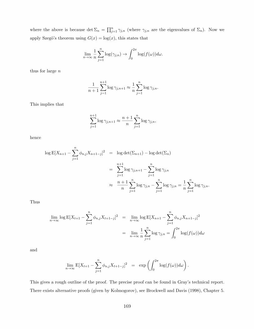
This gives a rough outline of the proof. The precise proof can be found in Gray’s technical report.
There exists alternative proofs (given by Kolmogorov), see Brockwell and Davis (1998), Chapter 5.
169
This is the reason that in many papers the assumption
Z
2⇡
0
log f(!)d! > �1
is made. This assumption essentially ensures Xt /2 X�1.
Example 5.8.1 Consider the AR(p) process Xt = �Xt�1
+ "t (assume wlog that |�| < 1) where
E["t] = 0 and var["t] = �2. We know that Xt(1) = �Xt and
E[Xt+1
�Xt(1)]2 = �2.
We now show that
exp
✓
1
2⇡
Z
2⇡
0
log f(!)d!
◆
= �2. (5.39)
We recall that the spectral density of the AR(1) is
f(!) =�2
|1� �ei!|2) log f(!) = log �2 � log |1� �ei!|2.
Thus
1
2⇡
Z
2⇡
0
log f(!)d! =1
2⇡
Z
2⇡
0
log �2d!| {z }
=log �2
� 1
2⇡
Z
2⇡
0
log |1� �ei!|2d!| {z }
=0
.
There are various ways to prove that the second term is zero. Probably the simplest is to use basic
results in complex analysis. By making a change of variables z = ei! we have