Chapter 5 Topological Graph Theory

§ 5.1. Basic Notations

Topological graph theory studies the ”drawing” of a graph on a surface.

A proper drawing on a surface of a graph G with |G| = p and ||G|| = q

follows the rules :

(1). There are p points on the surface which corresponds to the set of

vertices in G; and

(2). There are q curves joining points defined above which correspond

to the set of edges and they are pairwise disjoint except possibly for

the endpoints.

• The drawing is on a surface defined on R3.

• A 2-manifold is a connected topological space in which every point

has a neighborhood homeomorphic to the open unit disk defined on R2.

• An n-manifold is a connected topological space in which every point

has a neighborhood homeomorphic to Bn = {(x1, x2, ..., xn) ∈ Rn |n∑

i=1x2

i < 1}.

• A subspace M of R3 is bounded if there exists a positive real number

K such that M ⊆ {(x, y, z) | x2 + y2 + z2 = K}.• Let M ⊆ R3 be a 2-manifold. Then M is said to be closed if it is

bounded and the boundary of M coincides with M .

• Let M(⊆ R3) be a 2-manifold; M is said to be orientable if for

every simple closed C on M, a clockwise sense of rotation is preserved

by traveling once around C. Otherwise, M is non-orientable.

• A 2-manifold M is orientable if and only if it is two-sided.

1

Definition 5.1.1. (Orientable Surface)

A surface is a compact orientable 2-manifold that may be thought of

as a sphere on which has been placed(inserted) a number of ”handles”

(holes). A sphere, denoted by S0, is the surface of a 3-dimension ball.

More precisely, S0 = {(x, y, z)|x2 + y2 + z2 = r2, r ∈ R+}. S1 is known

as a torus, S2 a double torus, and Sh is a surface obtained by adding h

handles to S0.

Definition 5.1.2. (Non-Orientable Surface)

A surface obtained by adding k cross-caps to S0 is known as the non-

orientable surface Nk. (A cross cap is obtained from Mobius band

described in what follows.)

Cross cap: Attach the boundary of a Mobius band to a cycle on S0 to

obtain a cross cap.

d

ca

b

x

y

a d, b c, x y

Definition 5.1.3. (Embedding or Imbedding, 2-cell embed-

ding)

An embedding of a graph in a surface is a continuous 1-1 function from

a topological representation of the graph into the surface. If every

region of the embedding is homeomorphic to a 2-dim open disc, then

the embedding is a 2-cell embedding(圓盤嵌入).

2

Embedding of K5 on S1 Embedding of K3,3 on S1

Embedding of K5 on N1 Embedding of K3,3 on N1

(N1 is also known as a projective plane. )

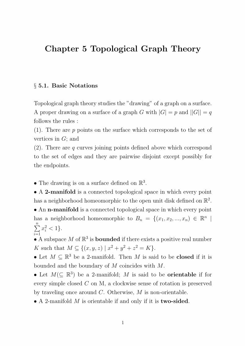
• Surfaces can be represented by a polygon (standard fundamental).

aa-1

aa

2-gon

3

4-gon

1 1 1 1

1 1 1 1aba b a b a b

1 1 1

1 1 2 2

1

1 2

( )( )

.

abab ab ab b b a a a a

where a ab and a b

4

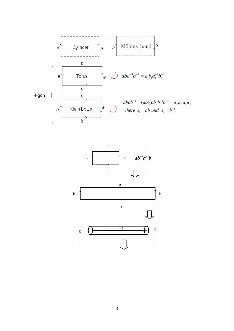
(*) The standard fundamental polygon for Sk is a1b1a−11 b−1

1 ...akbka−1k b−1

k .

(**) The standard fundamental polygon for Nh is a1a1a2a2...ahbh.

Definition 5.1.4. If a graph G can be embedded in S0, then G is

a planar graph.

Theorem 5.1.1.(Euler’s Formula)

Let G be a connected planar graph which has p vertices, q edges and

r regions. Then p − q + r = 2.

Proof. By induction on q. ¤

Corollary 5.1.2.

Let G be a planar graph which has k components, p vertices, q edges

and r regions. Then p − q + r = 1 + k.

Proof. By induction on k. k = 1 is true by Theorem 1. Assume the

assertion is true for k. Let G be a graph with p vertices, q edges and r

regions, and G have k+1(≥ 2) components. Now let G = G+e (e con-

nects two components). Then, G has p vertices, q + 1 edges, r regions

and k components. Hence, p−(q+1)+r = 1+k. This implies p−q+r =

1 + (k + 1). The proof follows. ¤

5

Definition 5.1.5. (Maximal planar graph)

A planar graph is maximal if ∀ u, v ∈ V (G), uv /∈ E(G), G + uv is not

planar.

Theorem 5.1.3. If G is a maximal planar (p, q)-graphs, then q =

3p − 6.

Proof. 3r = 2q, whenever G is maximal. ¤

Corollary 5.1.4. If G is a planar graph, then q ≤ 3p − 6.

Theorem 5.1.5. If G is a planar graph with girth g, then G has at

most gg−2(p − 2) edges, i.e., q ≤ g

g−2(p − 2).

Proof. gr ≤ 2q; p − q + r = 2; p − q + 2qq ≥ 2; p − 2 ≥ q(1 − 2

q );

p−2 ≥ q g−2g . ¤

Theorem 5.1.6. If G is a maximal planar graph (must be connected),

then 3p3 + 2p4 + p5 = p7 + 2p8 + · · · + (n − 6)pn + 12 (n = ∆(G)).

Proof. p =∑n

i=3 pi, 2q =∑n

i=3 ipi, q = 3p − 6, 3p3 + 2p4 + p5 ≥ 12

=⇒∑n

i=3 ipi = 6∑n

i=3 pi − 12. Now, the proof follows. ¤

• Every planar graph has at least one vertex of degree less than 6.

• Not every graph((p, q)-graph) with q = 3p − 6 is planar.

• If G is planar, then every subgraph is planar.

• Contracting an edge of a planar graph gives a planar graph.

G is planar=⇒ G/e is planar.

• Planar graphs and spherical graphs are planar graphs.

Definition 5.1.6. (Dual graph of planar graph)

The dual graph G∗ of a planar graph G is a plane graph whose ver-

tices correspond to the faces of G, whose edges xy correspond a common

edge of two regions x and y (in G).

6

G : p, q, r

G∗ : p∗, q∗, r∗

p∗ = r, q∗ = q, r∗ = p.

• The dual graph of a planar graph is also a planar graph.

• Some people like ”faces” than ”regions”.

Second Proof of Euler’s Formula (Pseudograph!!)

By induction on p. p = 1, G has q loops and q + 1 regions. p− q + r =

1 − q + (q + 1) = 2. done. Assume the assertion is true when p = n.

Let G be a graph with p = n + 1 vertices. Since G is connected and

p = n + 1 > 2, G has an edge e. Now, contracting e of G, we obtain a

graph G′ such that G′ has p − 1 vertices, q − 1 edges and r regions(?).

By hypothesis (p− 1)− (q − 1) + r = 2. Hence p− q + r = 2. ¤

Corollary 5.1.7 Every planar graph is 5-degenerate.

Theorem 5.1.8. Wagner[1936], Fary[1948] and Stein[1951]

Every (finite) planar graph G has an embedding in ”plane” where all

edges are straight line segments. (Known as Fary’s Theorem)

Proof. Let G be the graph which is maximally planar and G ≥ G.

Then, the proof follows by showing G can be embedded in plane such

that all edges are straight line segments. By induction on |G|.

~

| | 3G ,

~

| | 4,G

7

•••

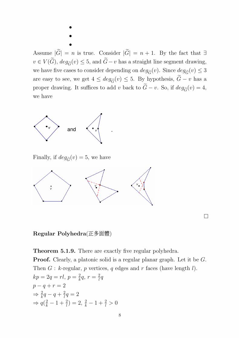
Assume |G| = n is true. Consider |G| = n + 1. By the fact that ∃v ∈ V (G), degG(v) ≤ 5, and G− v has a straight line segment drawing,

we have five cases to consider depending on degG(v). Since degG(v) ≤ 3

are easy to see, we get 4 ≤ degG(v) ≤ 5. By hypothesis, G − v has a

proper drawing. It suffices to add v back to G − v. So, if degG(v) = 4,

we have

vand v .

Finally, if degG(v) = 5, we have

.

¤

Regular Polyhedra(正多面體)

Theorem 5.1.9. There are exactly five regular polyhedra.

Proof. Clearly, a platonic solid is a regular planar graph. Let it be G.

Then G : k-regular, p vertices, q edges and r faces (have length l).

kp = 2q = rl, p = 2kq, r = 2

l q

p − q + r = 2

⇒ 2kq − q + 2

l q = 2

⇒ q(2k − 1 + 2

l ) = 2, 2k − 1 + 2

l > 0

8

⇒ 2l − kl + 2k > 0 ⇒ kl − 2k − 2l < 0

⇒ (k − 2)(l − 2) = kl − 2l − 2k + 4 < 4

Now, k ≤ 5 and thus l ≤ 5 (?) (Dual graph is also planar!).

By direct checking the graph exists if and only if

(k, l) = {(3, 3), (3, 4), (3, 5), (4, 3), (5, 3)}. This concludes the proof.

(k,l) q p r Name

(3,3) 6 4 4 Tetrahedron( )

(3,4) 12 8 6 Cube( )

(4,3) 12 6 8 Octahedron( )

(3,5) 30 20 12 Dodecahedron( )

(5,3) 30 12 20 Icosahedron( )

¤Definition 5.1.7. (Crossing Number)

The crossing number of G, cr(G), is defined to the minimum number

of crossings in a proper drawing of G on a plane.

• If G is a planar graph, then cr(G) = 0.

• If G is nonplanar, then cr(G) > 0.

• cr(K5) = 1, cr(K6) = 3.

• It is conjecture by Guy et al that cr(Kp) = 14b

p2cb

p−12 cbp−2

2 cbp−32 c and

the conjecture has been verified for p ≤ 10.

• (Conjecture) cr(Km,n) = bm2 cb

m−12 cbn

2cbn−1

2 c.The conjecture has been verified for 1 ≤ min{m,n} ≤ 6. (Kleitman)

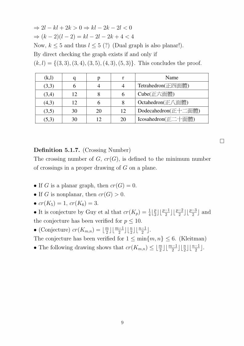
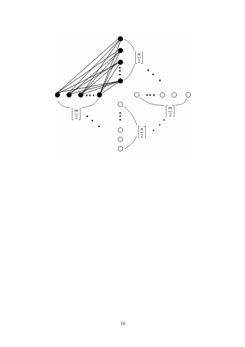
• The following drawing shows that cr(Km,n) ≤ bm2 cb

m−12 cbn

2cbn−1

2 c.

9

10

§ 5.2. Characterization of Planar Graphs

Definition 5.2.1. A subdivision of a graph is obtained from it by

replacing edges with pairwise internally disjoint paths.

Definition 5.2.2. A graph H is said to be homeomorphic from G if

either H ∼= G or H is isomorphic to a subdivision of G. A graph G1 is

homeomorphic with G2 if there exists a graph G3 such that G1 and G2

are both homeomorphic from G3.

Both of G1 and G2 are homeomorphic from G3.

1G

2G

3G

Proposition 5.2.1. If a graph G has a subgraph that is homeomor-

phic from K5 or K3,3 , then G is nonplanar.

Proof. Trivial.

In what follows, we shall prove that well-known theorem in character-

izing planar graphs.

11

Theorem 5.2.2. (Kuratowski [1930])

A graph is planar if and only if it does not contain a subgraph which

is homeomorphic from K5 or K3,3.

First, we need a couple of definitions.

Definition 5.2.3. A subdivision of K5 or K3,3 is called a Kuratowski

subgraph.

Definition 5.2.4. A minimal nonplanar graph is a nonplanar graph

such that every proper subgraph is planar.

• If F is the edge set of a region in a planar embedding (in S) of G,

then G has an embedding (in plane) with F being the edge set of the

unbounded region.

Lemma 5.2.3. Every minimal nonplanar graph G is 2-connected.

Proof. (By contraposition.)

planarplanar

(1). G is disconnected.

(2). G has a cut-vertex.

Definition 5.2.5. Let S be a set of vertices in a graph G. An S-lobe

12

of G is an induced subgraph of G whose vertex set consists of S and

the vertices of ”a” component of G − S.

Lemma 5.2.4. Let S = {x, y} be a separating 2-set of G. If G is

nonplanar, then adding the edge xy to some S-lobe of G yields a non-

planar graph.

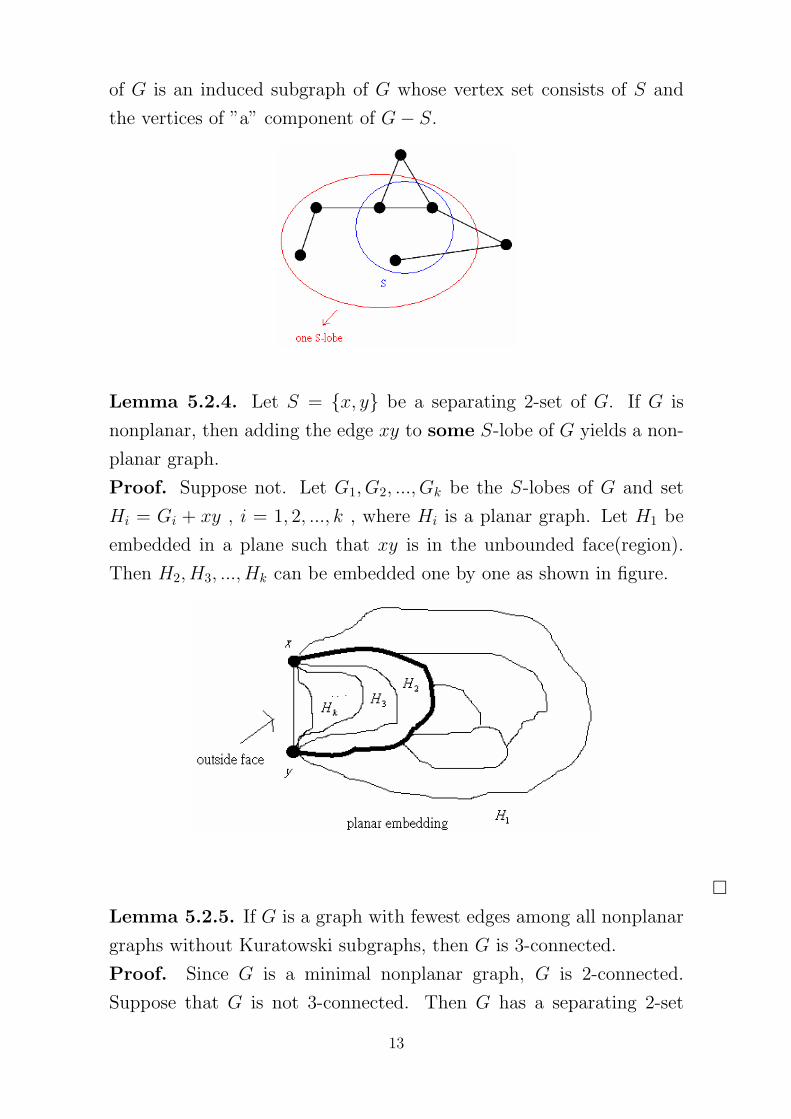
Proof. Suppose not. Let G1, G2, ..., Gk be the S-lobes of G and set

Hi = Gi + xy , i = 1, 2, ..., k , where Hi is a planar graph. Let H1 be

embedded in a plane such that xy is in the unbounded face(region).

Then H2, H3, ..., Hk can be embedded one by one as shown in figure.

¤Lemma 5.2.5. If G is a graph with fewest edges among all nonplanar

graphs without Kuratowski subgraphs, then G is 3-connected.

Proof. Since G is a minimal nonplanar graph, G is 2-connected.

Suppose that G is not 3-connected. Then G has a separating 2-set

13

S = {x, y}. Since G is nonplanar, there is an S-lobe H containing

xy which is also nonplanar. By assumption, H has a Kuratowski sub-

graphs, F , since ‖ H ‖<‖ G ‖. Now, if xy ∈ E(F ) then clearly F is

a Kuratowski subgraphs of G, a contradiction. On the other hand, if

xy ∈ F but xy /∈ E(G), then a subdivision of F is contained in G (see

the following figure).

¤Definition 5.2.6. A convex embedding of a graph is a planar embed-

ding in which each region boundary is a convex polygon.

Lemma 5.2.6. (Thomassen [1980])

Every 3-connected graph G with at least 5 vertices has an edge e such

that G/e (G · e) is 3-connected.

Proof. Let e = xy and the vertex obtained by shrinking e be xy. Now,

suppose that G/e is not 3-connected. Hence G/e has a separating 2-set

S. Clearly, xy ∈ S. Thus, let z be the other vertex in S. We call z,

the mate of xy. Observe that {x, y, z} is a separating 3-set of G. Since

every edge of G has a mate, (for otherwise the edge can be contracted

and the new graph is also 3-connected), let xy and z be chosen so that

the resulting disconnected graph G − {x, y, z} has a largest compo-

nent H. Let H ′ be another component in G − {x, y, z} (See figure).

Since {x, y, z} is a minimal separating set, each vertex in {x, y, z} has

a neighbor in each H and H ′. Let u be a neighbor of z in H ′ and v be

a mate of uz. By the definition of a mate, G−{u, z, v} is disconnected.

However, 〈V (H)∪ {x, y}〉G

is connected and for each vertex v′ in H ′ is

not a cut-vertex, for otherwise {z, v′} is a 2-separating set of G. This

implies that in G − {z, u, v} we have a component which is of order at

14

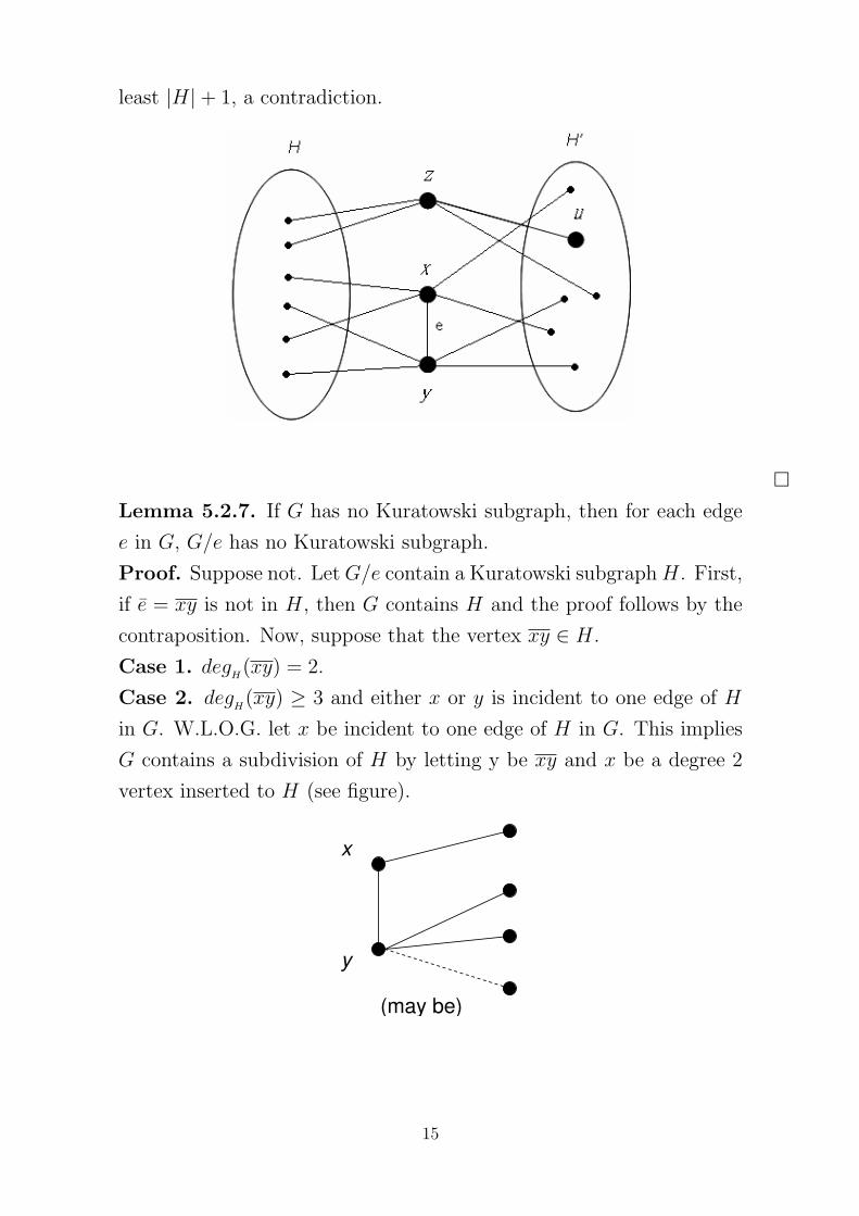
least |H| + 1, a contradiction.

¤Lemma 5.2.7. If G has no Kuratowski subgraph, then for each edge

e in G, G/e has no Kuratowski subgraph.

Proof. Suppose not. Let G/e contain a Kuratowski subgraph H. First,

if e = xy is not in H, then G contains H and the proof follows by the

contraposition. Now, suppose that the vertex xy ∈ H.

Case 1. degH(xy) = 2.

Case 2. degH(xy) ≥ 3 and either x or y is incident to one edge of H

in G. W.L.O.G. let x be incident to one edge of H in G. This implies

G contains a subdivision of H by letting y be xy and x be a degree 2

vertex inserted to H (see figure).

(may be)

x

y

15

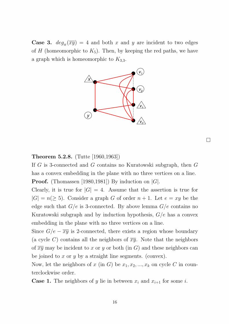
Case 3. degH(xy) = 4 and both x and y are incident to two edges

of H (homeomorphic to K5). Then, by keeping the red paths, we have

a graph which is homeomorphic to K3,3.

X

v1

v2

y

v1

v2

¤

Theorem 5.2.8. (Tutte [1960,1963])

If G is 3-connected and G contains no Kuratowski subgraph, then G

has a convex embedding in the plane with no three vertices on a line.

Proof. (Thomassen [1980,1981]) By induction on |G|.Clearly, it is true for |G| = 4. Assume that the assertion is true for

|G| = n(≥ 5). Consider a graph G of order n + 1. Let e = xy be the

edge such that G/e is 3-connected. By above lemma G/e contains no

Kuratowski subgraph and by induction hypothesis, G/e has a convex

embedding in the plane with no three vertices on a line.

Since G/e − xy is 2-connected, there exists a region whose boundary

(a cycle C) contains all the neighbors of xy. Note that the neighbors

of xy may be incident to x or y or both (in G) and these neighbors can

be joined to x or y by a straight line segments. (convex).

Now, let the neighbors of x (in G) be x1, x2, ..., xk on cycle C in coun-

terclockwise order.

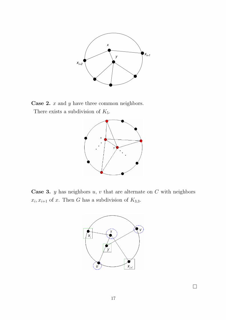
Case 1. The neighbors of y lie in between xi and xi+1 for some i.

16

x

yxi+1

xi+2

Case 2. x and y have three common neighbors.

There exists a subdivision of K5.

Case 3. y has neighbors u, v that are alternate on C with neighbors

xi, xi+1 of x. Then G has a subdivision of K3,3.

¤

17

Theorem 5.2.9. (Kuratowski [1930])

A graph is planar if and only if it does not contain a subdivision of K5

or K3,3.

Proof. (=⇒) If a graph does contain a subdivision of K5 or K3,3, then

the graph is not planar by using Euler’s Formula for K5 and a revised

version for K3,3.

(⇐=) If the graph does not contain a subdivision of K5 or K3,3 and it is

nonplanar, then we can delete some of its edges to obtain a 3-connected

”nonplanar” graph which contains no Kuratowski subgraphs. Then, by

Tutte’s Theorem for convex planar embedding, this graph must be pla-

nar, a contradiction. ¤

Theorem 5.2.10. (Schnyder [1990])

Every n-vertex planar graph has a straight-line embedding in which the

vertices are located at integer grid points in [0, n − 1] × [0, n − 1].

Proof. Omitted.

Definition 5.2.7. A graph H is a minor of a graph G if a copy of

H can be obtained from G by deleting ”or” contracting edges of G.

e.g. K5 is a minor of the Petersen graph but Petersen graph does

not contain a subdivision of K5.

• If G contains a subdivision of H, say H ′, then H is a minor of G.

We can also prove the following theorem.

Theorem 5.2.11. (Wagner [1937])

G is planar if and only if neither K5 nor K3,3 is a ”minor” of G.

e.g. Petersen graph is nonplanar.

18

§ 5.3. Graph Embeddings

Definition 5.3.1. The orientable genus of a graph G, γ(G), is the

minimum genus of a surface in which G can be embedded. The non-

orientable genus of a graph G, γ(G), is the minimum non-orientable

genus of a surface (crosscaps) in which G can be embedded.

e.g. γ(K5) = γ(K6) = γ(K7) = 1.

γ(K5) = 1 = γ(K3,3).

4

5

2

3

0

1

7 7

77

Theorem 5.3.1. (Euler-Poincare) (for pseudo-graphs)

Let G be a (p, q)-graph which has a 2-cell embedding in an orientable

surface of genus n. Then p − q + r = 2 − 2n where r is the number of

regions.

Proof. By induction on n and it is true for n = 0 which is a direct

consequence of Euler’s formula. Now, assume the assertion is true for

the surface with genus less than n and G is a graph which has an ori-

entable 2-cell embedding on Sn.

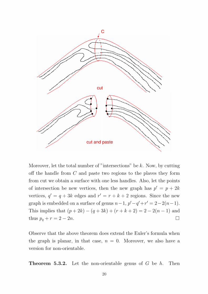
First, draw a cycle C along a handle which does not meet any vertex of

V (G), see figure below. Let C intersect m edges of G, see the following

figures.

19

cut

C

cut and paste

Moreover, let the total number of ”intersections” be k. Now, by cutting

off the handle from C and paste two regions to the plaves they form

from cut we obtain a surface with one less handles. Also, let the points

of intersection be new vertices, then the new graph has p′ = p + 2k

vertices, q′ = q + 3k edges and r′ = r + k + 2 regions. Since the new

graph is embedded on a surface of genus n−1, p′−q′+r′ = 2−2(n−1).

This implies that (p + 2k) − (q + 3k) + (r + k + 2) = 2 − 2(n − 1) and

thus pq + r = 2 − 2n. ¤

Observe that the above theorem does extend the Euler’s formula when

the graph is planar, in that case, n = 0. Moreover, we also have a

version for non-orientable.

Theorem 5.3.2. Let the non-orientable genus of G be h. Then

20

p − q + r = 2 − h.

Proof. Omitted.

Theorem 5.3.3. (The Rotational Embedding Scheme)

Let G be a nontrivial connected graph with V (G) = {v1, v2, ..., vp}. For

each 2-cell embedding of G on a surface, there exists a unique p-tuple

(π1, π2, ..., πp), where for i = 1, 2, ..., p, πi : V (i) −→ V (i) is a cyclic

permutation that describes the subscripts of the vertices adjacent to vi

in counterclockwise order about vi. Conversely, for each such p-tuple

(π1, π2, ..., πp), there exists a 2-cell embedding of G on some surface

such that for i = 1, 2, ..., p, the subscripts of the vertices adjacent to vi

and in counterclockwise order about vi are given by πi.

Key idea: π((vi, vj)) = π(vi, vj) = (vj, vπj(i)).

Proof. Omitted.

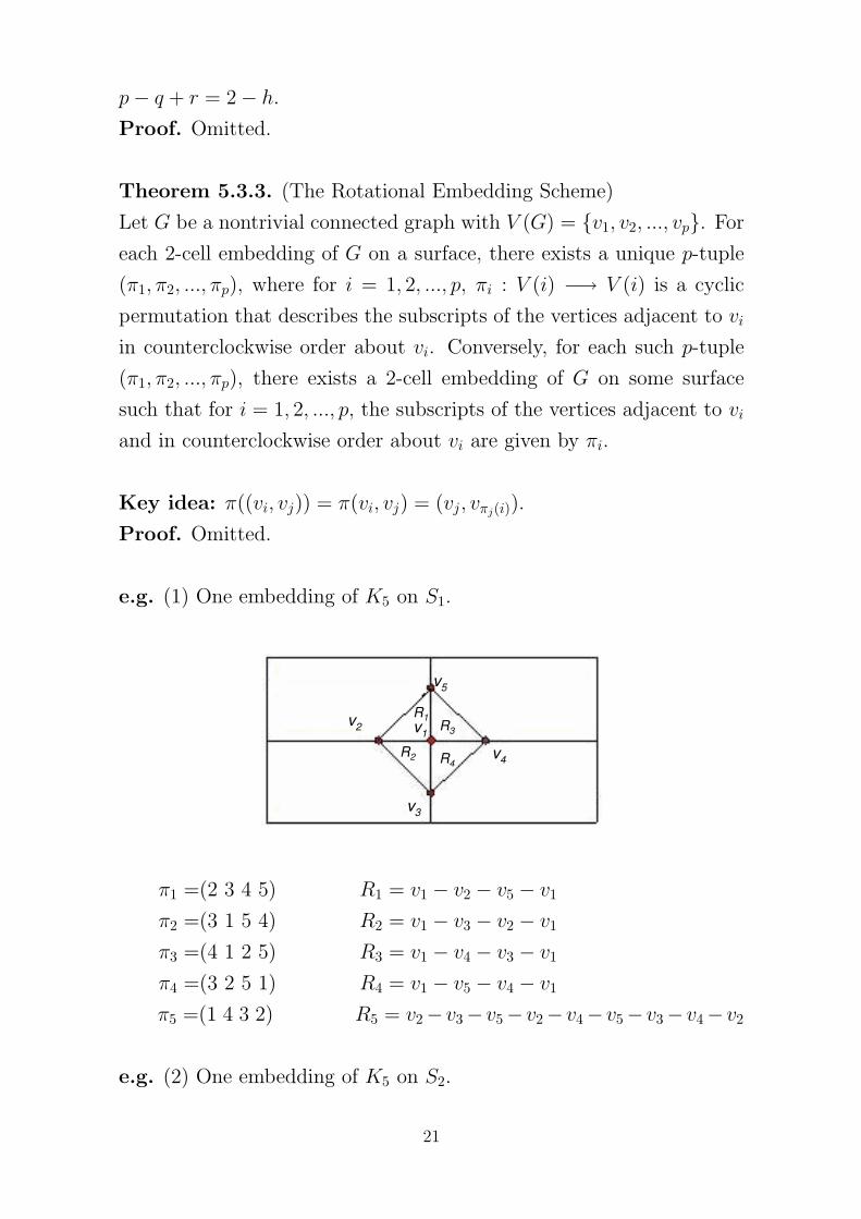
e.g. (1) One embedding of K5 on S1.

v5

v2

v3

v4

v1

R1

R2

R3

R4

π1 =(2 3 4 5) R1 = v1 − v2 − v5 − v1

π2 =(3 1 5 4) R2 = v1 − v3 − v2 − v1

π3 =(4 1 2 5) R3 = v1 − v4 − v3 − v1

π4 =(3 2 5 1) R4 = v1 − v5 − v4 − v1

π5 =(1 4 3 2) R5 = v2 − v3 − v5 − v2 − v4 − v5 − v3 − v4− v2

e.g. (2) One embedding of K5 on S2.

21

π1 =(3 2 4 5)

π2 =(3 1 5 4)

π3 =(4 1 2 5)

π4 =(3 2 5 1)

π5 =(1 4 3 2)

R1 = v1 − v2 − v5 − v1 − v3 − v2 − v1 − v4 − v3 − v1 − v2

R2 = v1 − v5 − v4 − v1 − v5

R3 = v2 − v3 − v5 − v2 − v4 − v5 − v3 − v4 − v2 − v3

e.g. (3) One embedding of K10,24 on S24.

Let A = {v1, v3, ..., v19} and B = {v2, v4, ..., v28}.Let π1 = π5 = π9 = π13 = π17 =def (2, 4, 6, ..., 28) (cycle)

π3 = π7 = π11 = π15 = π19 =def (28, 26, 24, ..., 2)

π2 = π6 = ... = π26 =def (1, 3, 5, ..., 19)

π4 = π8 = ... = π28 =def (19, 17, 15, ..., 1).

=⇒ Every region has 4 sides! Let’s see an example.

π(v7, v12) = (v12, vπ12

(7)) = (v12, v5)

π(v7, v12) = v7 − v12 − v5 − v14 − v7 − v12 = (v12, v5)

π(v12, v5) = (v5, vπ5(12)) = (v5, v14)

π(v5, v14) = (v14, vπ14

(5)) = (v14, v7)

π(v14, v7) = (v7, vπ7(14)) = (v7, v12)

We give the following result without a proof.

Theorem 5.3.4. (Interpolation Theorem, Duke [1966])

If there exist 2-cell embeddings of a connected graph G on surfaces Sm

and Sn where m < n and k is any integer m ≤ k ≤ n, then there exists

a 2-cell embedding of G on Sk.

So, it is interesting to know the maximum n such that G has a

22

2-cell embedding in Sn. Clearly, the largest possible value occurs when

the embedding has either one region or two regions depending on the

parity of p− q or equivalently q − p + 1, this is also known as the Betti

number of a (p, q)−graph.

We remark here that ”Interpolation Theorem” also holds for non-

orientable 2-cell embeddings.

Definition 5.3.2. (Maximum Genus)

The maximum genus γM(G) of G is the maximum among the genera of

all surfaces on which G can be 2-cell embedded.

• There arep∏

i=1(deg

G(vi) − 1)! p-tuples of a graph G.

⇒ γM(G) exists !

⇒ A connected graph G has a 2-cell embedding on Sk if and only if

γ(G) ≤ K ≤ γM(G).

• Finding γ(G) for a graph is very difficult, but finding γM(G) is com-

paratively easier.

Definition 5.3.3. (Betti Number of a Graph)

Let c(G) = k denote the number of components in G. Then, the Betti

number is defined to be β(G) = q − p + k. Thus, if G is connected,

then β(G) = q − p + 1.

• A tree has Betti number ”0”. So, if G is connected, β(G) ”mea-

sures” how far is G from a tree.

Theorem 5.3.5. If G is a connected graph, then γM(G) ≤ bβ(G)

2 c.Furthermore, equality holds if and only if there exists a 2-cell embed-

ding of G with 1 + δβ(G) regions where δ

β(G) =

{0 if β(G) is even ,

1 if β(G) is odd.

Proof. By Theorem 5.3.1., p − q + r = 2 − 2γM(G).

2γM(G) + r − 1 = q − p + 1 = β(G)

23

γM(G) = β(G)+1−r

2 ≤ β(G)2

⇒ γM(G) ≤ bβ(G)

2 c.

γM(G) = bβ(G)

2 c if and only if

{r = 1 if β(G) is even ,

r = 2 if β(G) is odd.¤

Definition 5.3.4. A (connected) graph G is upper embeddable if

γM(G) = bβ(G)

2 c.Definition 5.3.5. A spanning tree of a connected graph G is a split-

ting tree of G if at most one component of G−E(T ) has odd ”size”(邊

數).

Theorem 5.3.6. Let T be a splitting tree of a (p, q)-graph G. Then

every component of G−E(T ) has even size if and only if β(G) is even.

Proof. (⇒) G − E(T ) is of size q − p + 1 = β(G).

(⇐) Since at most one component of G−E(T ) is of odd size, the possible

one must be even too. ¤

Theorem 5.3.7. (Jungerman, Xuong, [1978,1979])

A graph G is upper embeddable if and only if G has a splitting tree.

Proof. A direct consequence of Theorem 5.3.9. ¤

Corollary 5.3.8. Let G be a graph which contains two edge-disjoint

spanning trees. Then G is upper embeddable.

Problem Which graph contains two edge-disjoint trees? 2 edge-connected?

3-connected? 4-edge-connected?

• γM(Kp) = b (p−1)(p−2)

4 c.• γ

M(Km,n) = b (m−1)(n−1)

2 c.• γ

M(Qn) = (n − 2)2n−2.

• γM(Km(n)) =?.

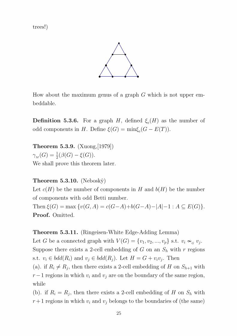
e.g. This graph is not upper emmeddable! (Contains no splitting

24

trees!)

How about the maximum genus of a graph G which is not upper em-

beddable.

Definition 5.3.6. For a graph H, defined ξ0(H) as the number of

odd components in H. Define ξ(G) = minξ0(G − E(T )).

Theorem 5.3.9. (Xuong,[1979])

γM(G) = 1

2(β(G) − ξ(G)).

We shall prove this theorem later.

Theorem 5.3.10. (Nebosky)

Let c(H) be the number of components in H and b(H) be the number

of components with odd Betti number.

Then ξ(G) = max {v(G,A) = c(G−A)+b(G−A)−|A|−1 : A ⊆ E(G)}.Proof. Omitted.

Theorem 5.3.11. (Ringeisen-White Edge-Adding Lemma)

Let G be a connected graph with V (G) = {v1, v2, ..., vp} s.t. vi �G

vj.

Suppose there exists a 2-cell embedding of G on an Sh with r regions

s.t. vi ∈ bdd(Ri) and vj ∈ bdd(Rj). Let H = G + vivj. Then

(a). if Ri 6= Rj, then there exists a 2-cell embedding of H on Sh+1 with

r−1 regions in which vi and vj are on the boundary of the same region,

while

(b). if Ri = Rj, then there exists a 2-cell embedding of H on Sh with

r+1 regions in which vi and vj belongs to the boundaries of (the same)

25

two distinct regions.

Proof. By direct checking. ¤

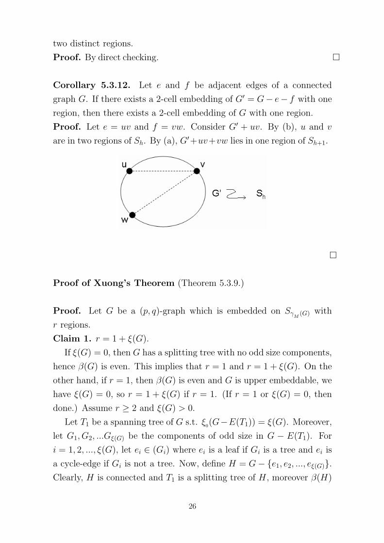
Corollary 5.3.12. Let e and f be adjacent edges of a connected

graph G. If there exists a 2-cell embedding of G′ = G− e− f with one

region, then there exists a 2-cell embedding of G with one region.

Proof. Let e = uv and f = vw. Consider G′ + uv. By (b), u and v

are in two regions of Sh. By (a), G′+uv+vw lies in one region of Sh+1.

¤

Proof of Xuong’s Theorem (Theorem 5.3.9.)

Proof. Let G be a (p, q)-graph which is embedded on SγM

(G) with

r regions.

Claim 1. r = 1 + ξ(G).

If ξ(G) = 0, then G has a splitting tree with no odd size components,

hence β(G) is even. This implies that r = 1 and r = 1 + ξ(G). On the

other hand, if r = 1, then β(G) is even and G is upper embeddable, we

have ξ(G) = 0, so r = 1 + ξ(G) if r = 1. (If r = 1 or ξ(G) = 0, then

done.) Assume r ≥ 2 and ξ(G) > 0.

Let T1 be a spanning tree of G s.t. ξ0(G−E(T1)) = ξ(G). Moreover,

let G1, G2, ...Gξ(G) be the components of odd size in G − E(T1). For

i = 1, 2, ..., ξ(G), let ei ∈ (Gi) where ei is a leaf if Gi is a tree and ei is

a cycle-edge if Gi is not a tree. Now, define H = G − {e1, e2, ..., eξ(G)}.Clearly, H is connected and T1 is a splitting tree of H, moreover β(H)

26

is even. Hence, H can be embedded on SγM

(H) with one region. Adding

the edges e1, e2, ..., eξ(G) back to H to obtain G. So, there exists a 2-cell

embedding of G on some surofaces with at most 1+ξ(G) regions. Since

G ↪→ SγM

(G) produces r regions, r ≤ 1 + ξ(G).

Now, assume that G is 2-cell embedded on SγM

(G) with r(≥ 2) regions.

Let f1 be an edge belonging to the boundary of two regions of G. Then

G − f1 ↪→ SγM

(G) with r − 1 regions. If r − 1 ≥ 2, continuing the

above process to obtain a graph G′ = G − {f1, f2, ..., fr−1} ↪→ SγM

(G)

with one region. Therefore, G′ has a splitting tree T ′. This im-

plies that G′ − E(T ′) contains only even size components and ξ(G) ≤ξ

0(G − E(T ′)) ≤ r − 1. Thus, r = 1 + ξ(G).

Now, by Euler-Poincare’s Theorem

p − q + r = 2 − 2γM(G)

2γM(G) = q − p + 1 − ξ(G) = β(G) − ξ(G)

γM(G) = 1

2(β(G)−ξ(G)). ¤

Note. β(G) − ξ(G) is always an even integer.

27

§ 5.4. Genus of Groups

We may use graph notion to give a picture of a group. It is known

that a group G can be obtained by using generators, i.e., every element

of G can be represented by a sequence (word) of g1, g2, ..., g−11 , g−1

2 , ...

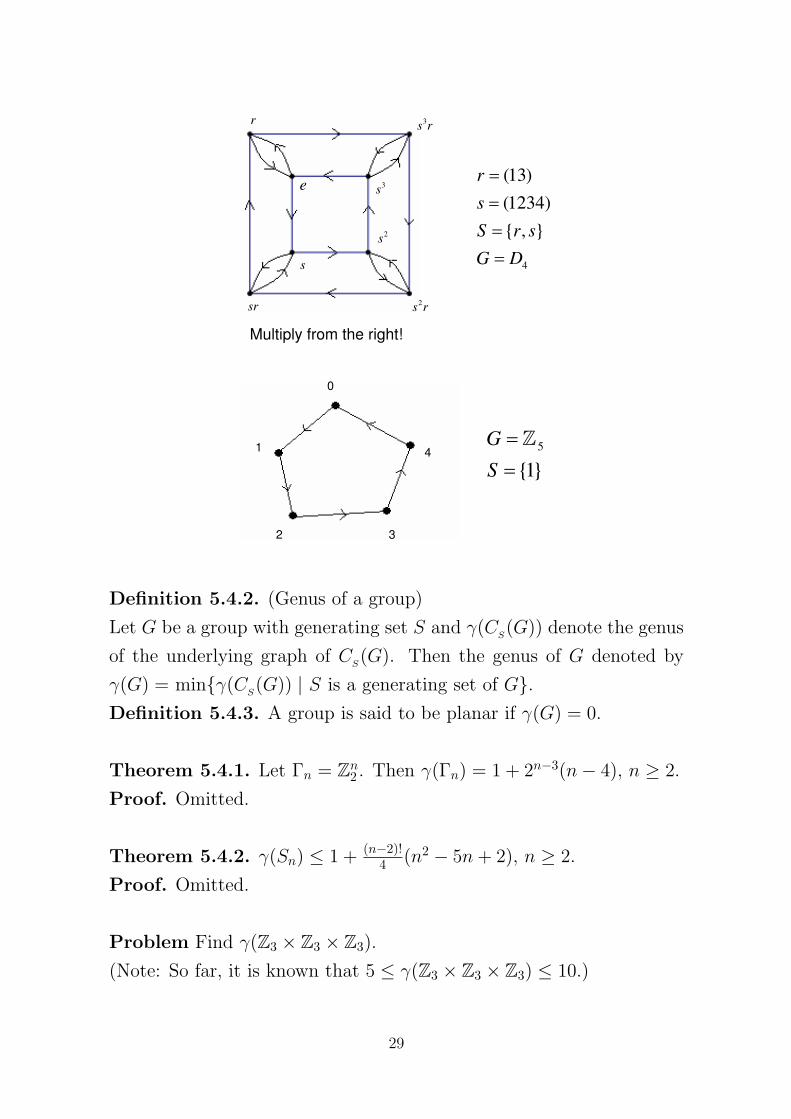
where g1, g2, ... are generators. For example, D4 can be generated by

{r = (13) and s = (1234)}.

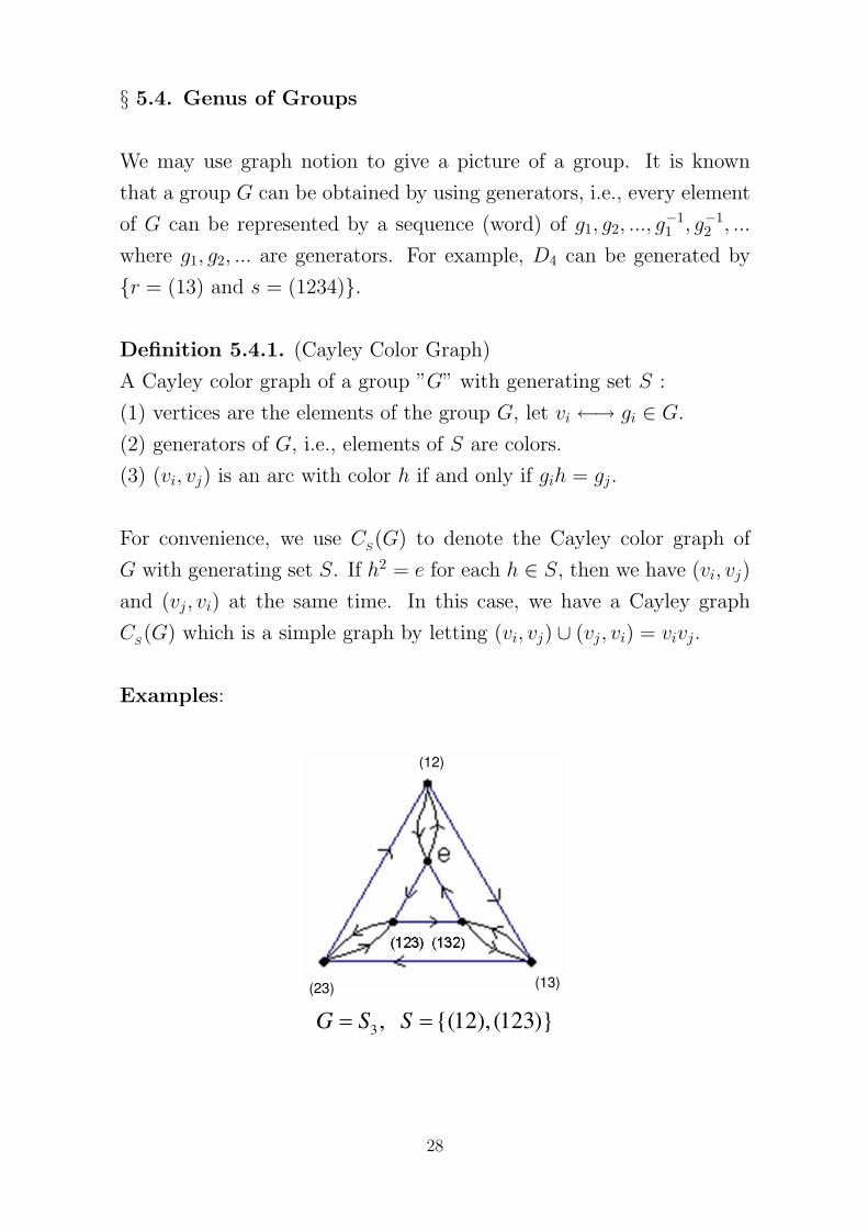
Definition 5.4.1. (Cayley Color Graph)

A Cayley color graph of a group ”G” with generating set S :

(1) vertices are the elements of the group G, let vi ←→ gi ∈ G.

(2) generators of G, i.e., elements of S are colors.

(3) (vi, vj) is an arc with color h if and only if gih = gj.

For convenience, we use CS(G) to denote the Cayley color graph of

G with generating set S. If h2 = e for each h ∈ S, then we have (vi, vj)

and (vj, vi) at the same time. In this case, we have a Cayley graph

CS(G) which is a simple graph by letting (vi, vj) ∪ (vj, vi) = vivj.

Examples:

3, {(12), (123)}G S S

(12)

(13)(23)

28

3s r

3s

2s

2s r

s

sr

e

Multiply from the right!

4

(13)

(1234)

{ , }

r

s

S r s

G D

r

0

1

2 3

45

{1}

G

S

Definition 5.4.2. (Genus of a group)

Let G be a group with generating set S and γ(CS(G)) denote the genus

of the underlying graph of CS(G). Then the genus of G denoted by

γ(G) = min{γ(CS(G)) | S is a generating set of G}.

Definition 5.4.3. A group is said to be planar if γ(G) = 0.

Theorem 5.4.1. Let Γn = Zn2 . Then γ(Γn) = 1 + 2n−3(n − 4), n ≥ 2.

Proof. Omitted.

Theorem 5.4.2. γ(Sn) ≤ 1 + (n−2)!4 (n2 − 5n + 2), n ≥ 2.

Proof. Omitted.

Problem Find γ(Z3 × Z3 × Z3).

(Note: So far, it is known that 5 ≤ γ(Z3 × Z3 × Z3) ≤ 10.)

29

§ 5.5. Selected Problem

Topological graph theory has been one of the most important topics

in the study of graph structures. Starting from the 4-color problem of

planar graphs, the progress of graph theory shows the importance of

researches in this topic. Almost all beautiful problems or conjectures

in graph theory are closely related to it. Clearly, we are not able to in-

clude all the problems here. Nevertheless, we shall list some of them in

this section. For convenience, the begining of each problem is marked

by ”•”.

• Thickness Problem

The thickness of a graph G is defined as the minimum number

of planar graphs in which G is decomposed, i.e., θ1(G) = min{n|G can

be decomposed into n planar graphs}. Clearly, the problem intends to

find θ1(G) for any given graph G. Some of the known results are:

(1). If G is a (p, q)-graph, then θ1(G) ≥ q(3p−6) .

(2). θ1(Kp) =

{bp+7

6 c if p 6= 9, 10; and ,

3 if p = 9, 10. (Beineke et al.)

(3). θ1(Qn) = bn+14 c.

(4). You may try to find θ1(Km(n)).

• Crossing Number Problem (Review)

The crossing number of a graph G, v(G), is defined to be the

minimum number of crossings in all drawings of G on a plane or corre-

spondingly a sphere. Clearly, we are interested in knowing v(G) for all

graphs of G. But, it turns out that this is also a very difficult problem.

Not much is known in general, people are working on special graphs.

Three of the most important ones are:

(1). Determine if v(G) = 14b

p2cb

p−12 cbp−2

2 cbp−32 c or not. (For p ≤ 10, it

30

is true.)

(2). Determine if v(Km,n) = bm2 cb

m−12 cbn

2cbn−1

2 c or not. (Some results

on small m and n have been obtained.)

(3). A good problem to try is finding v(Cm ×Cn). (It was conjectured

that v(Cm × Cn) = (m − 2)n when m ≤ n.)

• Genus Problem (Review)

The orientable (resp. non-orientable) genus of a graph G, γ(G) (resp.

γ(G)), is defined as the minimum number of handles of an orientable

(resp. non-orientable) surface in which G has an embedding on the

surface. Clearly, if the surface is Sk (resp. Nh), then γ(G) = k (resp.

γ(G) = h).

For example, γ(K5) = 1 and γ(K5) = 1. One of the most celebrating

theorems in graph genus in the following.

(1). γ(Kp) = d (p−3)(p−4)12 e, p ≥ 3. (Ringel and Youngs)

The result on Km,n is also outstanding.

(2). γ(Km,n) = b (m−3)(m−4)4 c, m,n ≥ 2. (Ringel)

(Note: Rotational scheme can be applied to prove (2).)

(3). Good problem to try : Find γ(Qn) and γ(Qn).

• Chromatic number of a surface

The chromatic number of a surface Sn, denoted by χ(Sn) is the

maximum chromatic number among all graphs that can be embedded

on Sn. So, the Four Color Theorem states that χ(S0) = 4. Heawood

proved χ(S1) = 7.

Theorem (The Heawood Map Coloring Theorem)

For every positive integer n, χ(Sn) = b7+√

1+48n2 c.

Proof. By the fact that γ(Kp) = d (p−3)(p−4)12 e and letting p = b7+

√1+48n2 c,

we conclude that χ(Sn) ≥ b7+√

1+48n2 c. Then, the proof follows by show-

31

ing χ(Sn) ≤ b7+√

1+48n2 c. This result has been done by Heawood long

time ago. We omit the detail here. ¤(1). Why n = 0 is not working?

(2). Can you prove the second inequality yourself?

• Book Embedding Problem

A page is a closed half-plane. A book is a collection of pages identi-

fied along the boundary of the half-planes. This common boundary is

called the spine. A book embedding is a drawing such that all vertices

lie on the spine and no edge contains a vertex on the spine other that

its ends. The page number of a graph G, pn(G), is the fewest number

of pages in a book embedding of G.

(1). For each positive integer n, pn(Cn) = 1.

(2). pn(K2,3) = 2. (?)

(3). Find pn(Km,n).

To conclude this chapter, we make the following comments:

(1). Find the genus (oriedtable or non-orientable) of a graph is going

to be very difficult, so far, no polynomial time algorithms have been

found. On the other hand, there exists a polynomial time algorithm to

find the maximum genus of a graph.

(2). Topological graph theory is an interesting topic but almost all

problems posed are very difficult to solve in general. So, special graphs

are the main ones which are of more attention.

32