Chapter 5

Traditional Analog ModulationTechniques

Mikael Olofsson — 2002–2007

Modulation techniques are mainly used to transmit information in a given frequency band.The reason for that may be that the channel is band-limited, or that we are assigned acertain frequency band and frequencies outside that band is supposed to be used by others.Therefore, we are interested in the spectral properties of various modulation techniques.

The modulation techniques described here have a long history in radio applications. Theinformation to be transmitted is normally an analog so called baseband signal. By that weunderstand a signal with the main part of its spectrum around zero. Especially, that meansthat the main part of the spectrum is below some frequency W , called the bandwidth ofthe signal.

We also consider methods to demodulate the modulated signals, i.e. to regain the originalsignal from the modulated one. Noise added by the channel will necessarily affect thedemodulated signal. We separate the analysis of those demodulation methods into onepart where we assume an ideal channel that does not add any noise, and another partwhere we assume that the channel adds white Gaussian noise.

5.1 Amplitude Modulation

Amplitude modulation, normally abbreviated AM, was the first modulation technique.The first radio broadcasts were done using this technique. The reason for that is that AMsignals can be detected very easily. Essentially, all you need is a nonlinearity. Actually,almost any nonlinearity will suffice to detect AM signals. There have even been reports ofpeople hearing some nearby radio station from their stainless steel kitchen sink. And some

67

68 Chapter 5. Traditional Analog Modulation Techniques

(including the author) have experienced that with a guitar amplifier. The crystal receiveris a demodulator for AM that can be manufactured at a low cost, which helped makingradio broadcasts popular.

In Chapter 3, Theorem 9, we noted that a convolution in the time domain corresonds to amultiplication in the frequency domain. In fact, the opposite is also true.

Theorem 10 (Fourier transform of a multiplication)Let a(t) and b(t) be signals with Fourier transforms A(f) and B(f). Then we have

F {a(t)b(t)} = (A ∗B)(f).

Proof: The proof is along the same line as the proof of Theorem 8, but starting with theinverse transform of the suggested spectrum. Based on our definitions, we have

F−1 {(A ∗B)(f)} =

∞∫

−∞

(A ∗B)(f)ej2πft df =

∞∫

−∞

∞∫

−∞

A(φ)B(f − φ) dφ ej2πft df.

We can rewrite the expression above as

F−1 {(A ∗B)(f)} =

∞∫

−∞

∞∫

−∞

A(φ)B(f − φ)ej2πft dφ df.

Now, set λ = f − φ, and we get

F−1 {(A ∗B)(f)} =

∞∫

−∞

∞∫

−∞

A(φ)B(λ)ej2π(λ+φ)t dτ dλ =

∞∫

−∞

A(φ)ej2πφt dφ

∞∫

−∞

B(λ)ej2πλt dλ.

Finally, we identify the last two integrals as the inverse Fourier transforms of A(f) andB(f), and we get

F−1 {(A ∗B)(f)} = a(t)b(t).

2

So, multiplying in the time domain corresponds to a convolution in the frequency domain.

5.1. Amplitude Modulation 69

3

2

1

0

−1

−2

−3−1 0 1

antenna

BP filter

diode

LP filter

ear-phone

3

2

1

0

−1

−2

−3−1 0 1

(a) (b) (c)

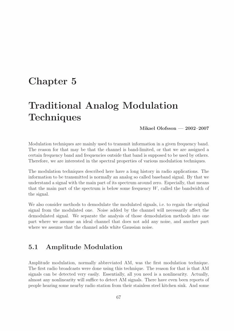
Figure 5.1: (a) A standard AM signal for the message m(t) = cos(2πt) with C = 2 and A = 1. Thedark line is C + m(t). (b) Principle of an envelope detector. (c) The correspondingoutput from an envelope detector.

Standard AM

An AM signal, x(t), corresponding to the message signal, m(t), is given by the equation

x(t) = A(C + m(t)) cos (2πfct) ,

where fc is referred to as the carrier frequency, A is some non-zero constant, and wherethe constant C is chosen such that |m(t)| < C holds for all t. In Figure 5.1a a standardAM signal is presented together with the message, which in this particular example is acosine signal.

We mentioned that AM signals can be detected using a nonlinearity. The first AM receiverwas the so called crystal receiver. It consists of an antenna, a resonance circuit (bandpassfilter), a diode and a simple low-pass filter. It extracts the envelope C + m(t) from x(t),and is therefore often called an envelope detector. The diode in Figure 5.1b is the non-linearity that makes the detection possible. The few simple components makes it possibleto manufacture the receiver at a low cost. In addition to that, it doesn’t even need a powersource of its own. The power is taken directly from the antenna. The output power is ofcourse very small, and only one listener could use the small earphone that was used. InFigure 5.1c, the AM signal is presented together with the output of an envelope detector.Note that the output is very similar to the original message. The mechanical parts inthe earphone, and the ear will further low-pass filter the output, so the listener will hearalmost the same signal as the one transmitted. Modern envelope detectors have amplifiersin various places and may be implemented digitally, but the basic construction is still abandpass filter, a diode (or some other rectifier) followed by a lowpass filter. An advantageof envelope detectors is that the BP filter that filters out everything except the intended

70 Chapter 5. Traditional Analog Modulation Techniques

Message

Carrier

Standard AM

|M(f)|

|F {cos(2πfct)}|

|X(f)|

1/21/2

lower sideband upper sidebandlower sidebandupper sideband

f

f

f

fc

fc

−fc

−fc

W−W

Figure 5.2: Spectrum for standard AM signals.

frequency band is not critical. It is enough if its center frequency is approximately correct.In other words, it does not need to know the carrier frequency exactly, or the carrier phasefor that matter.

We wish to study the spectrum of AM signals. Since an AM signal is the product of amessage and a carrier, that is easiest done based on Theorem 10. Thus, we need to findthe Fourier transform of cos(2πfct). First consider

F−1 {δ(f − fc)} =

∞∫

∞

δ(f − fc)ej2πft df = ej2πfct,

where the first equality is given by the definition of the inverse Fourier transform, andwhere the last equality is given by the definition of the unit impulse. So, we have

F {cos (2πfct)} = F{

ej2πfct + e−j2πfct

2

}

=1

2(δ(f − fc) + δ(f + fc)) .

Now we are ready to apply Theorem 10 on x(t). Let M(f) be the spectrum of m(t) andlet X(f) be the spectrum of x(t). Then we get

X(f) = F {AC cos (2πfct)}+ F {Am(t) cos (2πfct)}

=AC

2[δ(f − fc) + δ(f + fc)] +

A

2[M(f − fc) + M(f + fc)] .

5.1. Amplitude Modulation 71

It is left as an exercise to verify that the last equality holds. The involved spectraare displayed in Figure 5.2. Here AC

2(δ(f − fc) + δ(f + fc)) is referred to as the car-

rier, since that term corresponds to AC cos (2πfct). The other part of the spectrum,A2

(M(f − fc) + M(f + fc)), is referred to as the sidebands. Those sidebands are the onlyparts of the spectrum that depend on the message m(t). The sidebands are called upperand lower sidebands based on where they are compared to the carrier frequency, accordingto the following.

• Upper sideband : A2

(M(f − fc) + M(f + fc)) for |f | > fc.

• Lower sideband : A2

(M(f − fc) + M(f + fc)) for |f | < fc.

Because of those two sidebands, this type of AM modulation is often called double sideband

AM, abbreviated AM-DSB. There are also other versions of AM, but they cannot bedetected using an envelope detector.

Suppressed Carrier Modulation

All the information about the message m(t) in standard AM is in the sidebands. Thecarrier itself does not carry any information, and in that respect the carrier correspondsto unnecessary power dissipation. One version of AM that cannot be detected using anenvelope detector is called AM-SC or AM-DSB-SC, where SC should be interpreted asSuppressed Carrier. For this type of modulation, the constant C is simply set to zero, i.e.we have

x(t) = Am(t) cos (2πfct) ,

and the corresponding spectrum is

X(f) =A

2(M(f − fc) + M(f + fc)) .

So the carrier is removed from the spectrum, as the name suggests. In Figure 5.3, anAM-SC signal is presented together with the message and the corresponding envelopedetector output, as well as the absolute value of the message. Note that the output froman envelope detector in this case is close to the absolute value of the message. Thus, anenvelope detector cannot be used to receive AM-SC.

Demodulation of AM-SC can instead be done by modulating once more. Let y(t) withspectrum Y (f) be the output of that modulation. Then we have, similarily as above,

y(t) = x(t) cos (2πfct) = Am(t) cos2 (2πfct) =A

2m(t) (1 + cos(4πfct)) ,

72 Chapter 5. Traditional Analog Modulation Techniques

1

0

−1−1 0 1

1

0

−1−1 0 1

1

0

−1−1 0 1

(a) (b) (c)

Figure 5.3: (a) An AM-SC signal for the message m(t) = cos(2πt) with A = 1. The thick line ism(t). (b) The corresponding output from an envelope detector. (c) The AM-SC signaltogether with |m(t)| for comparison.

Message

AM-SC

Demodulated

|M(f)|

|X(f)|

|Y (f)|

f

f

f

fc−fc

2fc−2fc

W−W

Figure 5.4: Modulation of AM-SC and demodulation by modulating again.

5.1. Amplitude Modulation 73

and the corresponding spectrum is

Y (f) =A

2(X(f − fc) + X(f + fc)) =

A

2M(f) +

A

4(M(f − 2fc) + M(f + 2fc)) .

So, we have regained M(f), but we also have copies of M(f) centered around ±2fc. Theinvolved spectra are displayed in Figure 5.4. If W , the bandwidth of the message m(t),is smaller than fc, which normally is the case, then those copies do not overlap with theoriginal spectrum. Thus, we can use a suitable low-pass filter to remove the unwantedcopies. The further away the unwanted copies are in the frequency domain, the simplerthat filter can be. It should be noted that standard AM can also be demodulated usingthis method.

Single Sideband Modulation

Since there is a one-to-one relation between M(f) and M(−f), there is also a one-to-onerelation between the two sidebands, at least if W is smaller than fc. So, in both standardAM and AM-SC, we actually transmit our data twice in the frequency domain. No infor-mation is lost if we only transmit one of the sidebands. This type of AM is referred toas SSB, which should be interpreted as Single SideBand. There are SSB versions of bothstandard AM and AM-SC, and they can be obtained by first generating standard AMor AM-SC, and then using a suitable band-pass filter to remove the unwanted sideband.Spectra of AM-SSB and AM-SSB-SC are displayed in Figure 5.5. Obviously, SSB modula-tion only needs half the bandwidth compared to original AM or AM-SC. SSB-modulatedsignals can also be demodulated by modulating again using AM-SC, and we still get copiesnear ±2fc, that has to be removed by a low-pass filter. However these copies now containonly one sideband.

Synchronization for AM Demodulation

Demodulation by remodulation as described above is a method that can be used for detec-tion of all variants of AM. However, that demands that we have a correct carrier availablein the demodulator, with both correct frequency and at least approximately correct phase.For standard AM and for AM-SSB, where the carrier is available in the signal, it can easilybe extracted from the received signal using a narrow BP-filter with center frequency fc.For AM-SC, and for AM-SSB-SC, the absence of a carrier makes it impossible to extractthe carrier in that way. One way for the receiver to extract a carrier signal from an AM-SCsignal

x(t) = Am(t) cos (2πfct) ,

74 Chapter 5. Traditional Analog Modulation Techniques

AM-SSB

AM-SSB-SC |X(f)|

|X(f)|

upper sideband

upper sideband

f

ffc

fc

−fc

−fc

Figure 5.5: Spectra for AM-SSB and AM-SSB-SC.

NarrowLP filter

VCOcos(2πf0t)x(t) cos(φ)

2 cos(2πf0t + φ)

Figure 5.6: A phase-locked loop for generation of a well-defined carrier signal. The signal x(t) isgiven by x(t) = cos(2πf0t) cos(2πf0t + φ) = 1

2 (cos(4πf0t + φ) + cos(φ)). The devicelabelled VCO is a voltage controlled oscillator.

LP filter

LP filter

NarrowLP filter

VCO

phase shift

Am(t) cos(2πf0t)

Am(t) (cos(4πf0t + φ) + cos(φ))

Am(t) (sin(4πf0t + φ) + sin(φ))

Am(t) cos(φ)

Am(t) sin(φ)

A2m2(t) sin(2φ)∝ sin(2φ)

2 cos(2πf0t + φ)

2 sin(2πf0t + φ)

Figure 5.7: A Costas loop for detection of AM-SC.

5.1. Amplitude Modulation 75

is to produce the square

x2(t) = A2m2(t) cos2 (2πfct) =A2m2(t)

2(1 + cos (4πfct))

When we send information, the average of m2(t) is non-zero, which means that a scaledversion of cos (4πfct) can be extracted from x2(t), again using a narrow BP-filter, butwith center frequency 2fc. Extracting carriers in those ways will produce signals witha frequency that is the correct carrier frequency in the AM or AM-SSB case and twicethe carrier frequency in the AM-SC case, but the amplitude can vary from time to timedepending on the actual behaviour of the channel or the statistics of the information. Also,the extracted signal may include noise and parts of the sideband(s).

A clean carrier with both the correct frequency and a well defined amplitude, withoutany noise or residues from the sidebands, can be obtained from the extracted signal usinga phase-locked loop (PLL). There are several variants of phase-locked loops in use, anda simple variant is displayed in Figure 5.6. The signals given in Figure 5.6 assume thatthe input is already a clean sinusoid. In practice, the input is an extracted approximatecarrier which, as noted above, is polluted with noise and residues from the sidebands. Aphase-locked loop is a contol loop that produces a sinusoid with constant amplitude, thecorrect frequency f0 and an approximate phase φ. The voltage-controlled oscillator (VCO)is chosen such that the wanted carrier frequency corresponds to zero input. The frequencyfVCO(Vin) of the output of the VCO is a function of the input voltage Vin, such that thederivative of that function is positive, i.e. we have d

dVin

fVCO(Vin) > 0.

The carrier frequency in use may differ slightly from the wanted carrier frequency, and thephase-locked loop follows the carrier frequency, which means that the input to the VCOmay differ slightly from zero. In Figure 5.6 that means that the signal produced by the PLLhas phase φ for which cos(φ) ≈ 0 holds, in a point where cos(φ) has positive derivative.In other words, we have φ ≈ −π

2+ k · 2π for some integer k. We may assume any integer

value of k, since the produced signal is the same for different values of k. So, we can forinstance say that the signal has the phase φ ≈ −π

2.

For AM-SC, where we have squared the signal, and where the frequency of the extractedsignal is twice the carrier frequency, the feedback is equipped with a frequency doublerwhich can for instance be a squarer. The resulting output is then a sinusoid with thecorrect carrier frequency and phase approximately −π

4.

A special type of phase-locked loop that is especially well suited for detection of AM-SCsignals is the Costas loop, given in Figure 5.7. It extracts the carrier directly from thesignal. Again, the VCO is chosen such that the wanted carrier frequency corresponds tozero input. Thus, the loop produces a sinusoid whose frequency is the carrier frequencywith phase φ for which sin(2φ) ≈ 0 holds, in a point where sin(φ) has positive derivative.The resulting phase is therefore φ ≈ 0. The output of the Costas loop is the message m(t)scaled by cos(φ), but since we have φ ≈ 0, we also have cos(φ) ≈ 1.

76 Chapter 5. Traditional Analog Modulation Techniques

BP filter LP filterx(t) + noisex(t) + n(t)

2 cos(2πf0t)

Figure 5.8: Demodulation of AM signals in the presence of noise.

The reason that the Costas loop works is the presence of both sidebands, and the one-to-one mapping between the two sidebands. The two sidebands point at the carrier frequency,and the phase information in the sidebands gives us the carrier phase. The Costas loopcan therefore not be used for AM-SSB-SC. There is simply no way to extract the carrierfrom an AM-SSB-SC signal, due to the fact that the carrier is not available in the signal,and nothing in the spectrum gives any hint about the carrier frequency. That is the pricewe have to pay for suppressing both the carrier and one of the sidebands. Therefore, thereare a number of modifications of AM-SSB-SC, that makes it possible to extract a carrieranyway. The most simple method is not to suppress the carrier completely. Then the –however weak – carrier can be extracted from the signal. Another method is to send ashort carrier burst, and let a PLL lock on to that burst. After the burst, the oscillatorcontinues producing an internal carrier based on that burst. Of course, the oscillator willmost probably diverge from the used carrier eventually. Therefore the carrier burst isrepeated regularly. A third possibility is to keep a small part of the removed sideband, andin the receiver filter the other sideband similarily, and then extract a carrier using one ofthe methods above.

Impact of Noise in AM Demodulation

We would like to analyze the impact of noise on demodulation of AM signals. For thisanalysis we need to make some assumptions about the noise and about the demodulation.The first assumption is that the noise is dominated by thermal noise, and that it is inde-pendent of the message. As mentioned in Section 4.1, such noise can be modeled as whiteGaussian noise. We assume that the received signal is filtered by an ideal BP filter thatexactly matches the bandwidth of the AM signal before demodulation. We assume thatthe demodulation is done by remodulation by 2 · cos(2πf0t) as in the Costas loop. We alsoassume that the demodulated signal is filtered by an ideal LP filter that exactly matchesthe bandwidth of the message. See Figure 5.8.

We need to introduce some notation. Let W denote the bandwidth of the message. LetN0 denote the one-sided power spectral density of the assumed white Gaussian noise, andlet n(t) denote the noise after the BP filter. Also, introduce the following notation for theinvolved powers.

5.1. Amplitude Modulation 77

• P : The (expected) power of the message m(t).

• Pm−mod: The (expected) power of the received modulated signal x(t). Note that thismeans that A includes impacts of the channel.

• Pm: The (expected) power of the message after demodulation and LP filter.

• Pn−mod: The expected power of the ideally BP-filtered noise n(t) before demodula-tion.

• Pn: The expected power of the demodulated and LP-filtered noise.

We define the signal-to-noise ratio Pm/Pn after demodulation. We will compare this signal-to-noise ratio for DSB and SSB modulation using the same sent power Pm−mod transmittedover a channel with the same N0.

First we consider AM-SC. Then we have the signal

x(t) = Am(t) cos (2πfct)

with bandwidth 2W and expected power Pm−mod = A2P/2 since the carrier cos (2πfct)has average power 1/2. After demodulation, we regain Am(t), which means that we havePm = A2P . For the noise, we have Pn−mod = 2WN0. The demodulated noise

n(t) · 2 cos (2πfct)

has expected power 2Pn−mod, since the carrier 2 cos (2πfct) has average power 2. Half ofthat expected power is in the frequency interval |f | < W , while the other half is in thefrequency interval 2f0 −W < |f | < 2f0 + W . The latter part is removed by the LP filter,leaving us with Pn = Pn−mod. Finally, that gives us the signal-to-noise ratio

Pm

Pn

=A2P

2WN0

For AM-SSB-SC, one of the sidebands from AM-SC is removed, which means that thepower Pm−mod is reduced to half that of AM-SC. To produce an SSB signal with the samepower as in the DSB case, we therefore need to amplify the signal by

√2. So, we start

withx(t) =

√2Am(t) cos (2πfct) ,

and filter out one of the sidebands. Then we have the same sent power Pm−mod = A2P/2.After demodulation, we get a scaled version of the message. More precisely, the output isA√2m(t), which has power Pm = A2P/2. For the noise, we have Pn−mod = WN0, since the

bandwidth is W . The demodulated noise

n(t) · 2 cos (2πfct)

78 Chapter 5. Traditional Analog Modulation Techniques

still has expected power 2Pn−mod, since the carrier 2 cos (2πfct) has average power 2. Halfof that expected power is in the frequency interval |f | < W , while the other half is inthe frequency interval 2f0 −W < |f | < 2f0 + W . Actually, the other half of the poweris in the interval 2f0 −W < |f | < 2f0 if the lower sideband is used, or in the interval2f0 < |f | < 2f0 + W if the upper sideband is used. In any case, the part of the spectrumthat is near 2f0 is removed by the LP filter, leaving us with Pn = Pn−mod. Finally, thatgives us the signal-to-noise ratio

Pm

Pn

=A2P

2WN0

,

i.e. the same signal-to-noise ratio as for DSB.

5.2 Angle Modulation

Angle modulation is the common name for a class of modulation techniques, with that incommon that the bandwidth of the modulated signal is not given only by the bandwidthof the message, but also by a parameter called the modulation index. By setting thismodulation index to a suitable number, we can decide what bandwidth to use, and thelarger that index is, the better is the obtained quality. These methods, and combinationsof them are used in radio broadcasts in the FM-band (88–108 MHz).

The idea that angle modulation is based on is to let a function φ(m(t)) of the messagem(t) be the phase of a carrier, i.e. the sent signal is

x(t) = A · cos (2πfct + φ(m(t))) ,

where A is some non-zero constant, and where fc again is referred to as the carrier fre-quency. We say that φ(m(t)) is the momentary phase of x(t). Then the phase deviationφd(t) is the difference between the momentary phase and the average of the momentaryphase. Typically, m(t) has average zero, and the function f is chosen such that φ(m(t))also has average 0. Then we have

φd(t) = φ(m(t)),

and the peak phase deviation is defined as

φd,max = max |φd(t)|.

The peak phase deviation is also called the phase modulation index, and is denoted µp.

An alternative interpretation of the varying phase of the signal x(t), is to say that x(t) hasvarying frequency. We define the momentary frequency as

fmom(t) =1

2π· d

dt(2πfct + φ(m(t))) = fc +

1

2π· d

dtφ(m(t)).

5.2. Angle Modulation 79

Note, that this frequency is a function of time, just as the momentary phase also is afunction of time. The frequency deviation fd(t) is the difference between the momentaryfrequency and the carrier frequency, i.e.

fd(t) = fmom(t)− fc,

and the peak frequency deviation is defined as

fd,max = max |fd(t)|.

The frequency modulation index µf is defined as

µf =fd,max

W,

where W is the bandwidth of the message m(t), or rather the highest frequency componentin m(t). If m(t) is a stationary sine, then the two modulation indices are equal.

Spectrum of Angle Modulation

The spectra of angle modulated signals are generally hard to determine, due to the factthat angle modulation is non-linear. For the simple example

x(t) = A · cos (2πfct + µ sin(2πfmt)) ,

for fm ≪ fc, it is easily shown that µ is both the phase modulation index and the frequencymodulation index of that signal. It can also be shown that we have

x(t) =∞

∑

n=−∞

A · Jn(µ) cos (2π(fc + nfm)t) ,

where Jn(µ) is the Bessel function of order n. We will not at all try to perform that proof.The spectrum of that signal is

X(f) =∞

∑

n=−∞

A · Jn(µ)

2[δ(f + fc + nfm) + δ(f − fc − nfm)] .

The Bessel function of order n is given by

Jn(µ) =∞

∑

k=0

(−1)k

k!(n + k)!

(µ

2

)n+2k

for positive integers n. It can also be written as

80 Chapter 5. Traditional Analog Modulation Techniques

−0.5

0.5

1

µ0 2 4 6 8 10 12 14 16 18 20

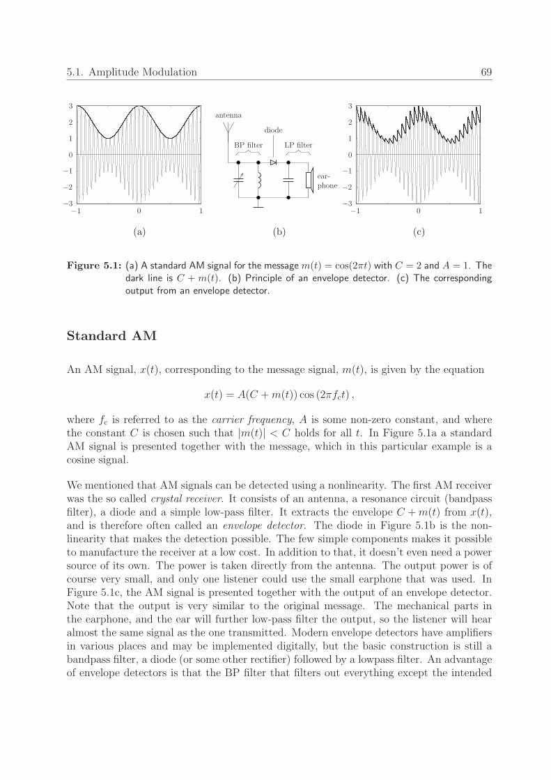
J0(µ)J1(µ) J2(µ) J3(µ) J4(µ) J5(µ) J6(µ) J7(µ)

Figure 5.9: Bessel functions Jn(µ) for n up to 7.

µ = 1

µ = 5

µ = 10

f

f

ffc

fc

fc

fm

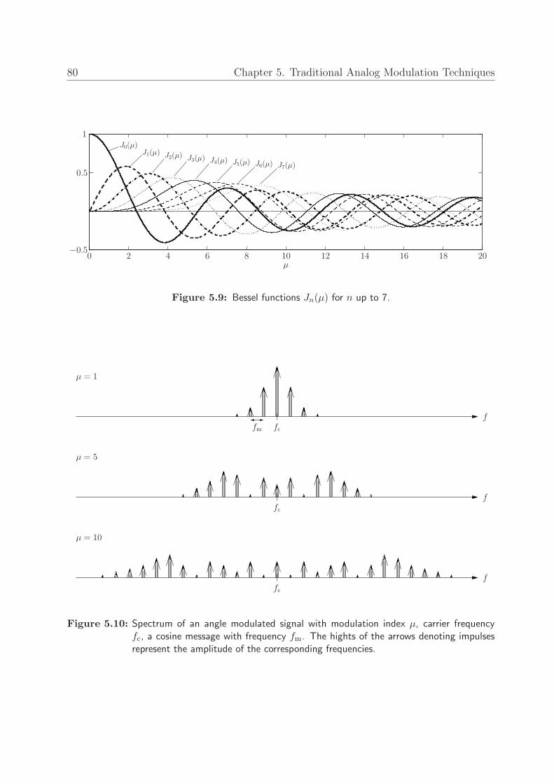
Figure 5.10: Spectrum of an angle modulated signal with modulation index µ, carrier frequencyfc, a cosine message with frequency fm. The hights of the arrows denoting impulsesrepresent the amplitude of the corresponding frequencies.

5.2. Angle Modulation 81

Jn(µ) =1

π

∫ π

0

cos(µ sin(φ)− nφ) dφ,

still for positive integers n. For negative integers n, we have

Jn(µ) = (−1)nJ−n(µ).

Formally, the bandwidth of this signal is infinite. However, the coefficients Jn(µ) decreaserapidly towards 0 for |n| > µ, see Figure 5.9. Thus, we can state that the bandwidth of thesignal is approximately 2µfm. A common approximation of the bandwidth is 2(µ + 1)fm,which is known as Carson’s rule. Using the identity µ = fd,max/fm, we can express the

bandwidth as 2(

1 + 1µ

)

fd,max. In Figure 5.10, we have plotted the spectra for three

different values of the modulation index µ, with a sine shaped message. Note how thebandwidth grows with the modulation index.

Phase Modulation

Phase modulation is normally abbreviated PM or PhM. The message, m(t), is in thistechnique used directly to determine the momentary phase, i.e. we have

φ(m(t)) = a ·m(t),

where a is some constant. The modulated signal, x(t), is thus given by

x(t) = A · cos (2πfct + a ·m(t)) .

The momentary frequency for this modulation is

fmom(t) =1

2π· d

dt(2πfct + a ·m(t)) = fc +

a

2π· d

dtm(t),

the frequency deviation is

fd(t) =a

2π· d

dtm(t).

and the peak frequency deviation is

fd,max =a

2π·max

∣

∣

∣

∣

d

dtm(t)

∣

∣

∣

∣

.

Finally, the frequency modulation index is given by

µf =a

2πW·max

∣

∣

∣

∣

d

dtm(t)

∣

∣

∣

∣

.

We notice that the peak frequency deviation depends on a · max∣

∣

ddt

m(t)∣

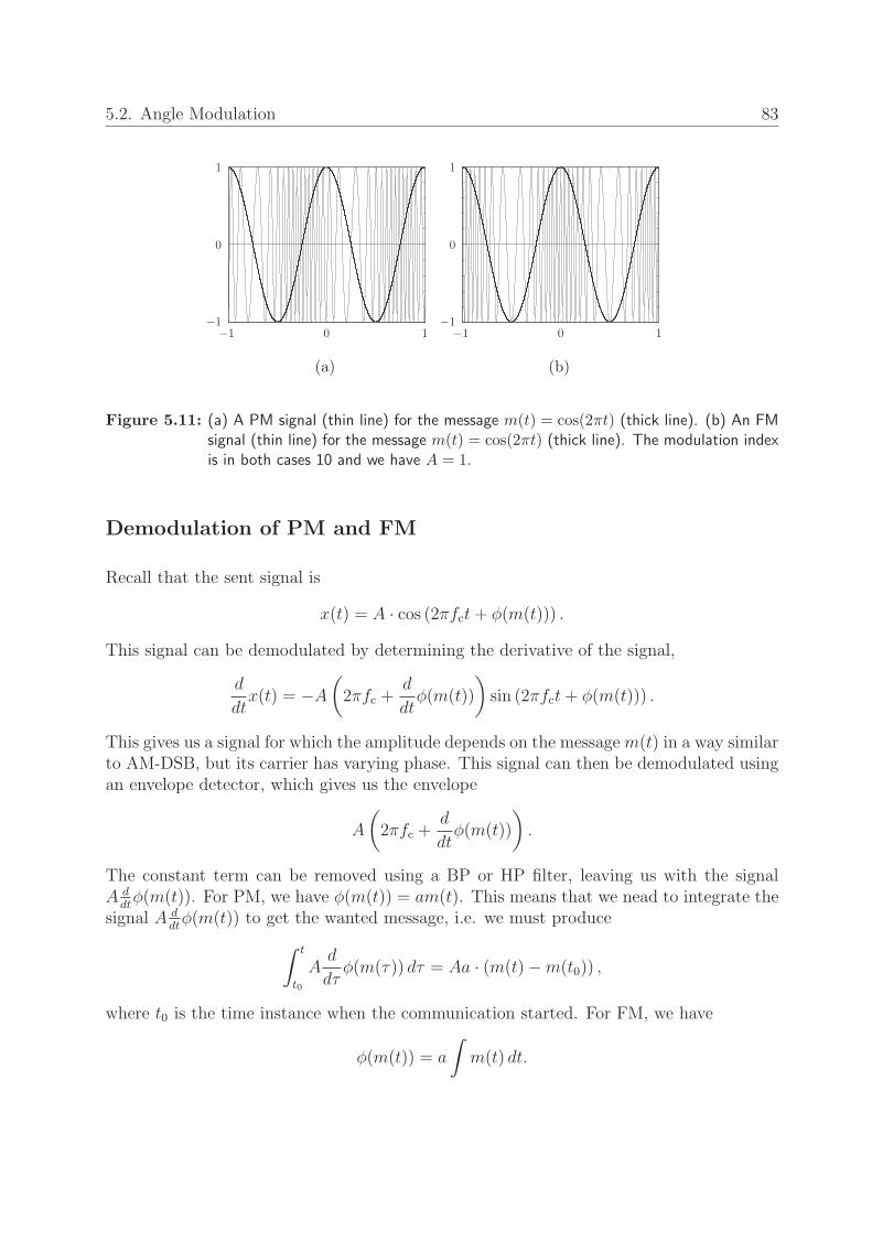
∣. Hence, thebandwidth of x(t) depends on the bandwidth of m(t), but also on the amplitude of m(t).In Figure 5.11a, a PM signal is presented together with the corresponding message.

82 Chapter 5. Traditional Analog Modulation Techniques

Frequency Modulation

Frequency modulation is normally abbreviated FM. As for PM, the message, m(t), deter-mines the phase of the carrier, but not directly. Instead, the derivative of the phase isproportional to m(t), i.e. the phase is a scaled indefinite integral of m(t). More precisely,we have

φ(m(t)) = a

∫

m(t) dt,

where a is some constant. The modulated signal, x(t), is then given by

x(t) = cos

(

2πfct + a

∫

m(t) dt

)

,

and the momentary frequency is given by

fmom(t) =1

2π· d

dt

(

2πfct + a

∫

m(t) dt

)

= fc +a

2π·m(t).

Thus, the momentary frequency is directly given by the message. Note that any indefiniteintegral of m(t) can be used as the phase. A natural choice is

φ(m(t)) = a

∫ t

t0

m(τ) dτ,

where t0 is the time instance when the communication starts. The frequency deviation is

fd(t) =a

2π·m(t).

and the peak frequency deviation is

fd,max =a

2π·max |m(t)|.

Finally, the frequency modulation index is given by

µf =a

2πB·max |m(t)|.

We notice that the frequency deviation depends on max |m(t)|. Hence, the bandwidth ofx(t) depends on the amplitude of m(t), but not on the bandwidth of m(t). In Figure 5.11b,an FM signal is presented together with the corresponding message.

5.2. Angle Modulation 83

1

0

−1−1 0 1

1

0

−1−1 0 1

(a) (b)

Figure 5.11: (a) A PM signal (thin line) for the message m(t) = cos(2πt) (thick line). (b) An FMsignal (thin line) for the message m(t) = cos(2πt) (thick line). The modulation indexis in both cases 10 and we have A = 1.

Demodulation of PM and FM

Recall that the sent signal is

x(t) = A · cos (2πfct + φ(m(t))) .

This signal can be demodulated by determining the derivative of the signal,

d

dtx(t) = −A

(

2πfc +d

dtφ(m(t))

)

sin (2πfct + φ(m(t))) .

This gives us a signal for which the amplitude depends on the message m(t) in a way similarto AM-DSB, but its carrier has varying phase. This signal can then be demodulated usingan envelope detector, which gives us the envelope

A

(

2πfc +d

dtφ(m(t))

)

.

The constant term can be removed using a BP or HP filter, leaving us with the signalA d

dtφ(m(t)). For PM, we have φ(m(t)) = am(t). This means that we nead to integrate the

signal A ddt

φ(m(t)) to get the wanted message, i.e. we must produce

∫ t

t0

Ad

dτφ(m(τ)) dτ = Aa · (m(t)−m(t0)) ,

where t0 is the time instance when the communication started. For FM, we have

φ(m(t)) = a

∫

m(t) dt.

84 Chapter 5. Traditional Analog Modulation Techniques

ddt

Envelopedetector BP filter

∫ t

t0x(t) A ·m(t)

Figure 5.12: Demodulation of PM.

ddt

Envelopedetector BP filterx(t) A ·m(t)

Figure 5.13: Demodulation of FM.

sgn(x) ddt

|x| LP filterx(t) ∝ fmom(t)

Figure 5.14: Detection of momentary frequency in angle modulated signals using zero crossings.

Then we have the signal

Ad

dtφ(m(t)) = A

d

dta

∫

m(t) dt = Aa ·m(t).

Therefore, demodulation of PM and FM can be done as indicated in Figures 5.12 and 5.13,respectively.

Alternatively, PM and FM can be demodulated by extracting the momentary frequency ofthe modulated signal x(t). That can be done by detecting the zero crossings of x(t). Thedemodulator in Figure 5.14 is based on this approach. The first block outputs the sign ofits input, i.e. its output is sgn(x(t)). The sgn function is defined as

sgn(x) =

1, x > 0,0, x = 0,-1, x < 0.

In practice, this block is an amplifier with very high gain. The second block producesthe derivative of its input. The result is that the output of the second block is a positive(negative) impulse when x(t) passes zero with positive (negative) derivative. After thethird block, which is a rectifier, all those impulses are positive, with momentary frequencythat is twice the momentary frequency of x(t). All that is left to produce the message is anLP filter, which is the last block in Figure 5.14. This produces a signal that is proportionalto the momentary frequency fmom(t) of x(t). For FM this is essentially the message m(t),and for PM this is essentially d

dtm(t). All we have left to do is to remove the DC component

5.2. Angle Modulation 85

that originates from the carrier frequency, using a HP filter, or by replacing the LP filterin Figure 5.14 by a BP filter. For PM, we also have to integrate the output to get themessage.

Impact of Noise in PM and FM Demodulation

We assume that the demodulation is carried out as described above, and we assume thatthe noise is dominated by white Gaussian noise with one-sided power spectral density N0.We use the same notation for the involved powers as we did for AM demodulation.

• P : The (expected) power of the message m(t).

• Pm−mod: The average power of the modulated signal x(t).

• Pm: The (expected) power of the message after demodulation and LP filter.

• Pn−mod: The expected power of the ideally BP-filtered noise before demodulation.

• Pn: The expected power of the demodulated and LP-filtered noise.

The signal x(t) is a cosine with amplitude A. The average power Pm−mod of the modulatedsignal x(t) is therefore given by Pm−mod = A2/2. The varying phase - or frequency for thatmatter - is irrelevant in this respect. For both PM and FM, the demodulated signal isAa ·m(t), which gives us Pm = A2a2P . The bandwidth of x(t) is approximately 2fd,max.The expected power Pn−mod of the ideally BP-filtered noise before demodulation is thereforePn−mod = 2fd,maxN0/2 = fd,maxN0.

Angle modulation methods are non-linear. That makes the analysis of detection in thepresence of noise a lot more complicated than for AM. We simply skip that analysis andstate the noise power for the two cases, under the assumption that the signal-to-noise ratioon the channel Pm−mod/Pn−mod is high.

We start with PM. Then it can be shown that the noise power is given by

Pn = 2WN0.

This gives us the signal-to-noise ratio

Pm

Pn

=A2a2P

2WN0

.

We would like to express this signal-to-noise ratio using the phase modulation index µp.We get

µp = max |φ(m(t))| = a ·max |m(t)|,

86 Chapter 5. Traditional Analog Modulation Techniques

from which we get

a =µp

max |m(t)| .

We use this relation to rewrite the signal-to-noise ration as

Pm

Pn

=

(

µp

max |m(t)|

)2A2P

2WN0

.

As we can see, we get increased signal-to-noise ratio with increased phase modulationindex.

Now we turn to FM. It can be shown that the noise power is given by

Pn =2W 3N0

3.

This gives us the signal-to-noise ratio

Pm

Pn

=A2a2P

2W 3N0/3.

Now we would like to express the signal-to-noise ratio using the frequency modulationindex µf . We have already noted that we have

µf =a ·max |m(t)|

2πW,

from which we geta

W=

2πµf

max |m(t)| .

We use this relation to rewrite the signal-to-noise ratio as

Pm

Pn

= 12π2

(

µf

max |m(t)|

)2A2P

2WN0

.

Here we get increased signal-to-noise ratio with increased frequency modulation index.

Pre-emphasized FM

The resulting noise after demodulating PM signals is evenly distributed over frequenciesfrom 0 to W , which resembles the situation for AM. That is not the case for FM, whereinstead the resulting noise is dominated by high frequencies (near W ). More precisely, thepower spectral density of the resulting noise after demodulating FM as described above is2N0f

2, where f is frequency. Therefore, if we could combine PM and FM in such a way thatPM is used for high frequencies in the message m(t) and FM is used for low frequencies,

5.2. Angle Modulation 87

we could hope for reduced noise compared to any of the two methods by themselves. Sucha combination exists and is called pre-emphasized FM. Then the message is first filteredusing a pre-emphasis filter with frequency response

H1(f) = 1 + jf/f0.

The output of that filter is then frequency modulated. In the receiver, after ordinarydemodulation of the FM signal, the result is filtered with an inverse filter of H1(f) calleda de-emphasis filter. That filter has frequency response

H2(f) =1

H1(f)=

1

1 + jf/f0

.

The result is that we regain the original signal, and that the resulting noise is smaller thanif we would have used ordinary PM or FM. The transmissions on the so called FM band(88-108 MHz) are done using pre-emphasized FM with f0 = 2122 Hz.