Chapter 6 Applications of the Laplace Transform

01(0 ) ( )Cv i dC

λ λ−

−

−∞

= ∫

In analyzing the circuit , we first wrote down the differential equation using KVL

Initial condition

Taking Laplace Transform for both side

were

Inverse Back

( )i t

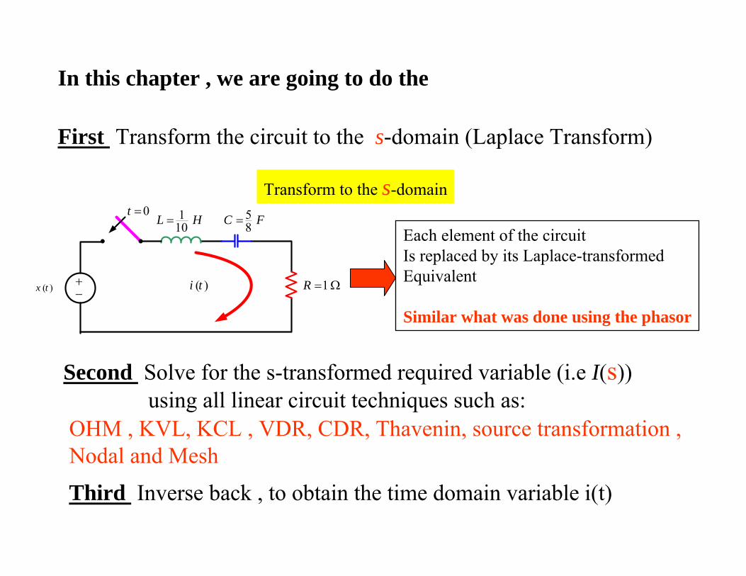
In this chapter , we are going to do the

Transform to the s-domain

Each element of the circuitIs replaced by its Laplace-transformedEquivalent

Similar what was done using the phasor

Transform)Laplacedomain (-sTransform the circuit to the First

))s(Ii.etransformed required variable (-Solve for the sSecondusing all linear circuit techniques such as:

)i(tInverse back , to obtain the time domain variable Third

OHM , KVL, KCL , VDR, CDR, Thavenin, source transformation , Nodal and Mesh

+−

1 R = Ω( ) i t

0 t = 1 10L H= 5 8C F=

( )x t

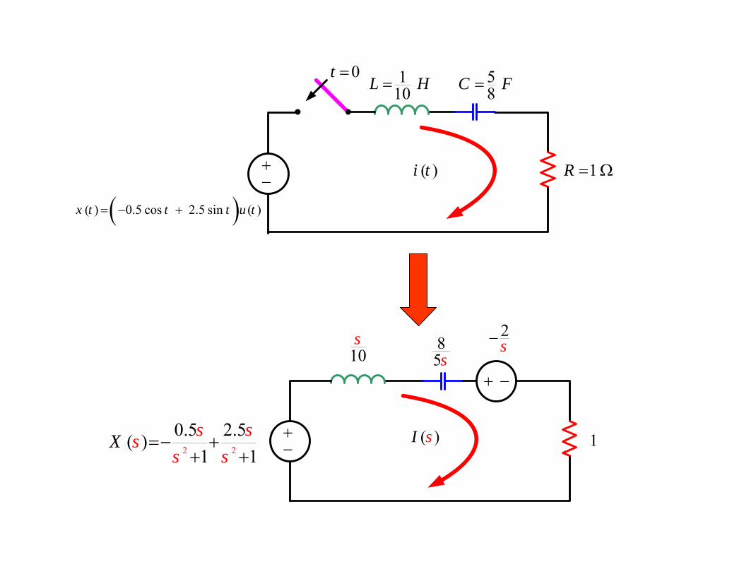
Example 6-1

R1 Z 1 R = Ω =⇒ Ω

2 2

0.5 2.5( ) ( )1 1

ssx t X ss s

=− ++ +

⇒

(0 ) 2 Cv V− = −(0 ) 0 Li V− =

L1 Z 10 10L H s= =⇒ Ω

C5 8 Z 58 F sC =⇒= Ω

+−

1 R = Ω

( )( ) 0.5 cos 2.5 sin ( )x t t t u t= − +

( ) i t

0 t = 110L H= 5 8C F=

10s

+−

8 5s+ −

1

2s−

2 2

0.5 2.5( )1 1

X s sss s

=− ++ +

( ) I s

+−

1 R = Ω

( )( ) 0.5 cos 2.5 sin ( )x t t t u t= − +

( ) i t

0 t = 110L H= 5 8C F=

10s

+−

8 5s+ −

1

2s−

2 2

0.5 2.5( )1 1

X s sss s

=− ++ +

( ) I s

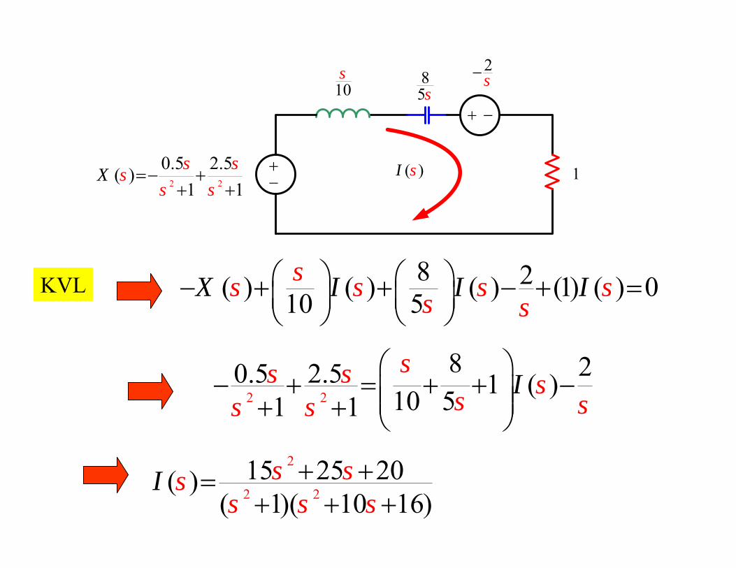
KVL 8 2( ) ( ) ( ) (1) ( ) 010 5X Iss s s ss sI I⎛ ⎞ ⎛ ⎞− + + − + =⎜ ⎟ ⎜ ⎟

⎝ ⎠ ⎝ ⎠

2 2

8 20.5 2.5 1 ( )10 51 1I

ss s ss ss s⎛ ⎞

− + = + + −⎜ ⎟⎜ ⎟+ + ⎝ ⎠2

2 215 25 20( )

( 1)( 10 16)s ss

s s sI + +=

+ + +

10s

+−

85s

+ −

1

2 s−

2 2

0.5 2.5( )1 1

X s sss s

=− ++ +

( ) I s

2

2 215 25 20( )

( 1)( 10 16)s ss

s s sI + +=

+ + +

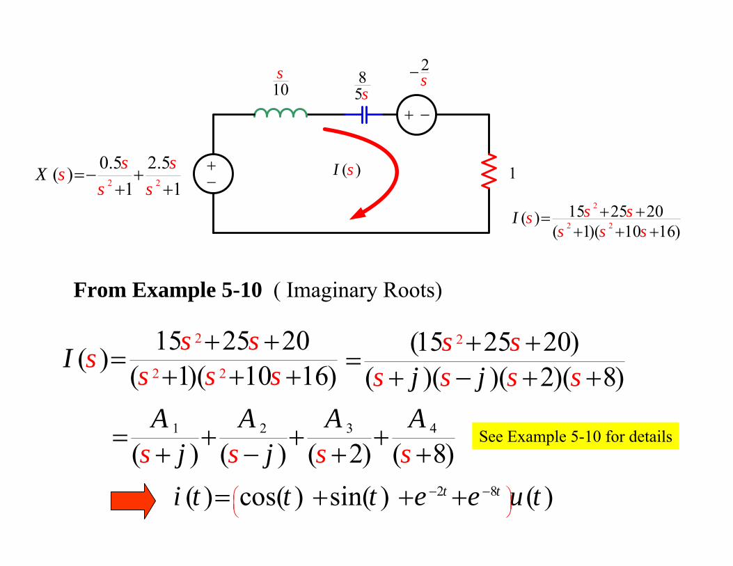
From Example 5-10 ( Imaginary Roots)

2

2 2

15 25 20( ) ( 1)( 10 16)s ss s s sI + +

=+ + +

2(15 25 20)( )( )( 2)( 8)j

s ss js s s

+ +=

+ − + +

1 2 3 4

( ) ( ) ( 2) ( 8)s s sA A A A

j sj= + + ++ − + +

2 8( ) cos( ) sin( ) ( )t ti t t t e e u t− −⎛ ⎞⎜ ⎟⎝ ⎠

= + + +

See Example 5-10 for details

6-4 Transfer FunctionsConsider the following circuit

+−

R( )x t ( ) i t

L

C

( )y t

+

−

input output

We want a relation (an equation) between the input x(t) and output y(t)

1( ) ' '( ) ( ) + ( )

tdi tx t L Ri t i t dtdt C

−∞

= + ∫KVL

2

2

( ) ( ) ( )( ) + dx t di t i tdi tL Rdt dt Cdt

= +

+−

R( )x t ( ) i t

L

C

( )y t

+

−

input output

2

2

( ) ( ) ( )( ) + dx t di t i tdi tL Rdt dt Cdt

= +

( )Since ( )

y ti t

R=

2

2

( ) ( ) ( )( ) + dx t L dy t y tdy t Rdt R dt RCdt

= +⇒

Writing the differential equation as 2

2

( ) ( )( ) + ( ) dx t dy tdy tRC LC RC y tdt dtdt

= +

+−

R( )x t ( ) i t

L

C

( )y t

+

−

input output

2

2

( ) ( )( ) + ( ) 1RC dx t dy tdy t y tdt dtd

LCt

RC= +

Real coefficients, non negative which results from system components R, L, C

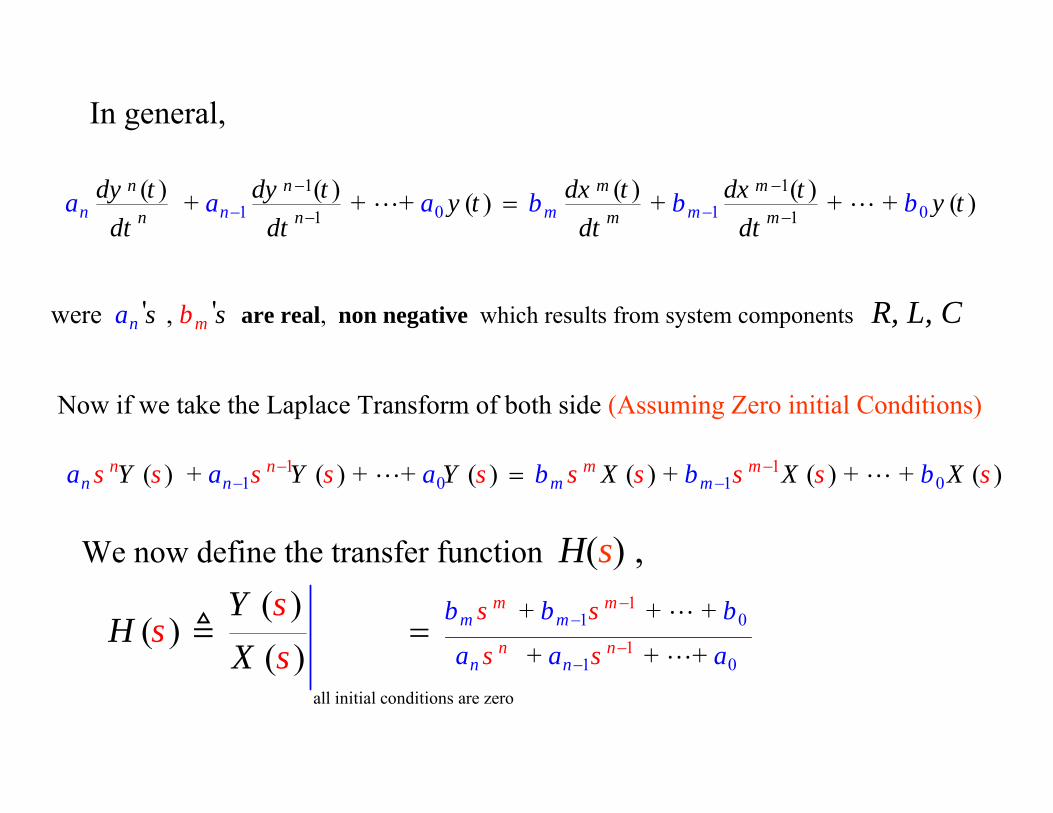
In general,

1 11 0 1 01 1

( ) ( ) ( ) ( ) + + + ( ) + + + ( )n n m m

n n m mn n m mdy t dy t dx t dx ty t y t

dt dt dt da a b b

ta b

− −

− −− −=

' 'were , n ms ba s are real, non negative which results from system components R, L, C

Now if we take the Laplace Transform of both side (Assuming Zero initial Conditions)

1 01

11

0( ) + ( ) + + ( ) ( ) + ( ) + + ( )n nn m

mn m

ma a a b bs s s s s s s s s sY Y bY X X X−− −

−=

We now define the transfer function H(s) ,

all initial conditions are zero

( )( )

( )Y

HX

ss

s1 0

1

11 0

+ + +

+ + + m m

n

m m

n nn

b b b

a a a

s s

s s −

−

−

−

=

1 11 0 1 01 1

( ) ( ) ( ) ( ) + + + ( ) + + + ( )n n m m

n n m mn n m mdy t dy t dx t dx ty t x t

dt dt dt da a b b

ta b

− −

− −− −=

1 01

1 0

1+ + +

+ + +

( )( ) ( )m

m

nm

n n

m

n

b b b

sa

s

as a

sYH ssXs

−−

−−

=

' 'Sin ce , n ms ba s are real, non negative

( ) ( )N sD s

The roots of the polynomials N(s) , D(s) are either real oroccur in complex conjugate

The roots of N(s) are referred to as the zero of H(s) ( H(s) = 0 )

The roots of D(s) are referred to as the pole of H(s) ( H(s) = ± ∞ )

The Degree of N(s) ( which is related to input) must be less than orEqual of D(s) ( which is related to output) for the system to be Bounded-input, bounded-output (BIBO)

( ) ( )N sD s

1 01

1 0

1+ + +

+ + +

( )( ) ( )m

m

nm

n n

m

n

b b b

sa

s

as a

sYH ssXs

−−

−−

=

Example :3 2

24 + 2 1

6 8( ) s s

ss

ssH + +

+ +=

Using polynomial division , we obtain 219 174 + 2 +

6 8( ) ss

s ssH − +

+ +=

Now assume the input x(t) = u(t) (bounded input) 1( ) s sX⇒ =

2

2 1 19 174 + + 6 8

( ) ( ) ( ) ss s s s

Y Xs s sH ⎛ ⎞⎜ ⎟⎜ ⎟⎝ ⎠

− ++ +

= =

1

219 174 ( ) + 2 +

( 6 8)( ) st

s s sy t Lδ

⎛ ⎞⎜ ⎟⎜ ⎟⎜ ⎟⎝ ⎠

− − ++ +

= unbounded

)

(

→ ∞

We see that for finite boundedInput (i.e x(t) =u(t) )We get an infinite (unbounded)output

for m n≤ BIBO

( ) ( )N sD s

1 01

1 0

1+ + +

+ + +

( )( ) ( )m

m

nm

n n

m

n

b b b

sa

s

as a

sYH ssXs

−−

−−

=

The poles of H(s) must have real parts which are negative

The poles must lie in the left half of the s-plan

Components of System Response

Consider the following differential equation ( Input / Output ),

1 0 0 ( ) ( ) ( ) dy t ya a bt x tdt + =

Taking Laplace Transform of both side,

1 0 0( ) (0 ) + ( ) )] ([ Y y Ya a bs s s sX−− =

1 0 10 ( ) ( ) (0[ )]s s sa Y X ya b a −− = +

1

1 0

0 ( ) (0 )( )

[ ] b as

aY

as

sX y −+

=−

1

1 0 1 0

0 (0 )

( ) ( ) + [ ] [ ]

s ss s

yb aa a a a

Y X−

=− −

1 0 0 ( ) ( ) ( ) dy t ya a bt x tdt + =

1

1 0 1 0

0 (0 )

( ) ( ) + [ ] [ ]

s ss s

yb aa a a a

Y X−

=− −

1 0

0

[ ]( ) ( )

Y

bs

a asX s=

−

all initial conditions are zero

( ) ( )( ) ( )( ) Y Ns sHX

s sDs

=1 0

0

][

sb

a a=

−

1

(0 )( ) ( ) ( ) +

( )s s

sy

Y H sXD

a −=

( ) ( ) ( ) + ( )sCH Xs

Ds

s=

A polynomial related to initial conditions

Transfer FunctionAll initial conditions are zeros

If initial conditions are zeros

1 0 0 ( ) ( ) ( ) dy t ya a bt x tdt + =

1

1 0 1 0

0 (0 )

( ) ( ) + [ ] [ ]

s ss s

yb aa a a a

Y X−

=− −

1

(0 )( ) ( ) ( ) +

( )s s

sy

Y H sXD

a −=

( ) ( ) ( ) + ( )sCH Xs

Ds

s=

A polynomial related to initial conditions

Transfer FunctionAll initial conditions are zeros

1 1 ( ) ( ) +

( )( [ ] ) ( )s sH X

sCy t L L D s

− − ⎡ ⎤⎢ ⎥⎣ ⎦

=

( ) ( ) + ( )y t y t y t=ZSR ZIR

Zero State Response

(Steady State)Zero State Response

(Steady State)

Example 6-7