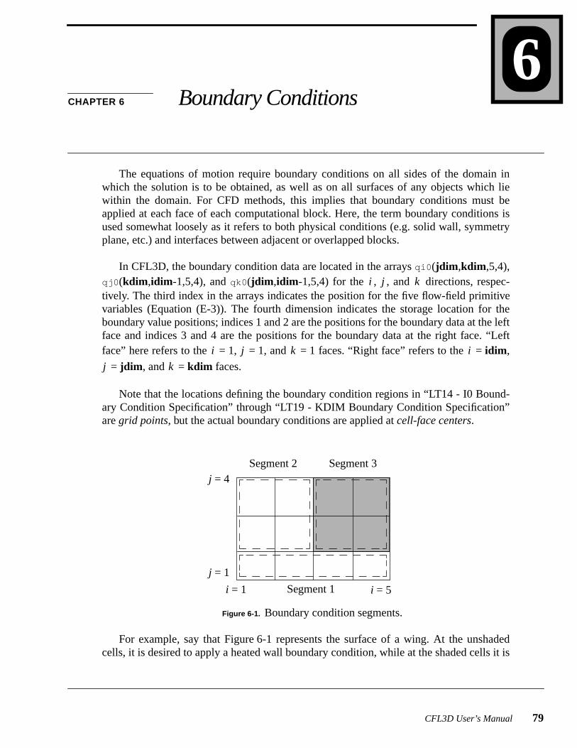
CHAPTER 6 Boundary Conditions - CFL3D

CFL3D User’s Manual 79

6CHAPTER 6 Boundary Conditions

The equations of motion require boundary conditions on all sides of the domain inwhich the solution is to be obtained, as well as on all surfaces of any objects which liewithin the domain. For CFD methods, this implies that boundary conditions must beapplied at each face of each computational block. Here, the term boundary conditions isused somewhat loosely as it refers to both physical conditions (e.g. solid wall, symmetryplane, etc.) and interfaces between adjacent or overlapped blocks.

In CFL3D, the boundary condition data are located in the arraysqi0(jdim,kdim,5,4),qj0(kdim,idim-1,5,4), andqk0(jdim,idim-1,5,4) for the , , and directions, respec-tively. The third index in the arrays indicates the position for the five flow-field primitivevariables (Equation (E-3)). The fourth dimension indicates the storage location for theboundary value positions; indices 1 and 2 are the positions for the boundary data at the leftface and indices 3 and 4 are the positions for the boundary data at the right face. “Leftface” here refers to the= 1, = 1, and = 1 faces. “Right face” refers to the = idim,

= jdim, and = kdim faces.

Note that the locations defining the boundary condition regions in “LT14 - I0 Bound-ary Condition Specification” through “LT19 - KDIM Boundary Condition Specification”aregrid points, but the actual boundary conditions are applied atcell-face centers.

For example, say that Figure6-1 represents the surface of a wing. At the unshadedcells, it is desired to apply a heated wall boundary condition, while at the shaded cells it is

Figure 6-1. Boundary condition segments.

i j k

i j k i

j k

i = 1 i = 5

j = 1

j = 4 Segment 2 Segment 3

Segment 1

CHAPTER 6 Boundary Conditions

80 CFL3D User’s Manual

desired to apply an adiabatic wall boundary condition. One way to accomplish this objec-tive would be to divide theK0 boundary condition into three segments, as indicated by thedashed lines in the figure. The CFL3D input file would look like this:

Line Type18 K0: GRID SEGMENT BCTYPE ISTA IEND JSTA JEND NDATA

1 1 2004 1 5 1 2 2twtype Cq1.6 0.0

1 2 2004 1 3 2 4 2twtype Cq1.6 0.0

1 3 2004 3 5 2 4 2twtype Cq0.0 0.0

Note that, for example, thegrid points to 5, to 2 define the boundary of thecells at which the boundary condition type for segment 1 is applied.

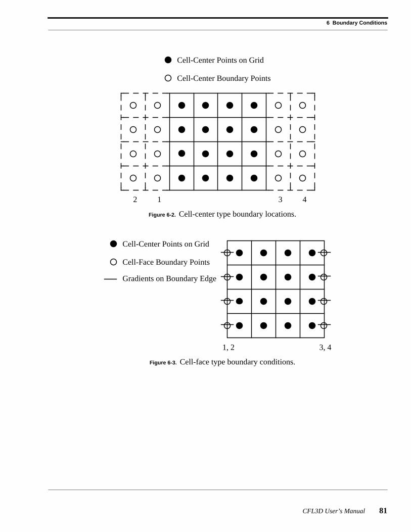
Two types of boundary condition representations are employed in CFL3D, namely,cell-center and cell-face. For cell-center type boundary conditions, the flow-field variablesare specified at “ghost” points corresponding to two cell-center locations analyticallyextended outside the grid as illustrated in Figure6-2. For example,qi0( , ,l,1) contains

the boundary data at the ghost point locations right next to the = 1 cell-center data and

qi0( , ,l,2) contains the boundary data in the second set of ghost point locations at the

left boundary. Likewise,qi0( , ,l,3) contains the boundary data at the ghost point loca-

tions right next to the = idim cell-center data andqi0( , ,l,4) contains the boundarydata in the second set of ghost point locations at the right boundary. The same boundarydata location definitions apply for theqj0 andqk0 arrays.

For cell-face type boundary conditions, the flow-field variables and their gradients arespecified at the cell-face boundary as illustrated in Figure6-3. For cell-face type boundaryconditions,qi0( , ,l,1) contains the flow-field variable data at the= 1 grid cell-face and

qi0( , ,l,2) contains the flow-field variable gradients at the= 1 grid cell-face. Likewise,

qi0( , ,l,3) contains the flow-field variable data at the = idim grid cell-face and

qi0( , ,l,4) contains the flow-field variable gradients at the= idim grid cell-face. Thesame boundary data location definitions apply for theqj0 andqk0 arrays.

Note that when running in 2-d mode (i2d = 1), it does not matter what boundary con-ditions are used on the= 1 and = idim faces (provided that the boundary conditionitself does not require more than one interior cell).Bctype is generally set to 1002 onthese faces.

Boundary conditions for the eddy viscosity are stored invi0, vj0, andvk0, whileboundary conditions for the field equation turbulence models are stored inti0, tj0, andtk0. Both of these are cell-center type, although only the first ghost points (1 and 3) areused. The field equation turbulence model boundary conditions are described in moredetail in SectionH.7 on page296.

i 1= j 1=

j k

i

j k

j k

i j k

j k i

j k i

j k i

j k i

i i


6 Boundary Conditions

Figure 6-2. Cell-center type boundary locations.

Figure 6-3. Cell-face type boundary conditions.

Cell-Center Points on Grid

Cell-Center Boundary Points

12 3 4


Cell-Face Boundary Points

Gradients on Boundary Edge

1, 2 3, 4



6.1Physical Boundary Conditions

The 1000 series of boundary condition types are used for physical boundary condi-tions and are specified at any of a block’s six faces in “LT14 - I0 Boundary ConditionSpecification” on page32 through “LT19 - KDIM Boundary Condition Specification” onpage35. In each case,ndata = 0, since no additional information is required for imple-mentation of the condition. The 1000 series boundary condition types currently supportedare as follows:

6.1.1Free Stream

bctype 1000

The free stream boundary conditions are cell-center type boundary conditions. Thefive flow-field variables for both sets of ghost points are set equal to the initial values,which are:

(6-1)

where .

bctype boundary condition1000 free stream1001 general symmetry plane1002 extrapolation1003 inflow/outflow1004 (no longer available, use 2004 instead)1005 inviscid surface1008 tunnel inflow1011 singular axis – half-plane symmetry1012 singular axis – full plane1013 singular axis – partial plane

ρini tial 1.0=

uini tial M∞ α βcoscos=

vini tial M– ∞ βsin=

wini tial M∞ α βcossin=

pini tial ρini tial aini tial( )2 γ⁄=

aini tial 1.0=


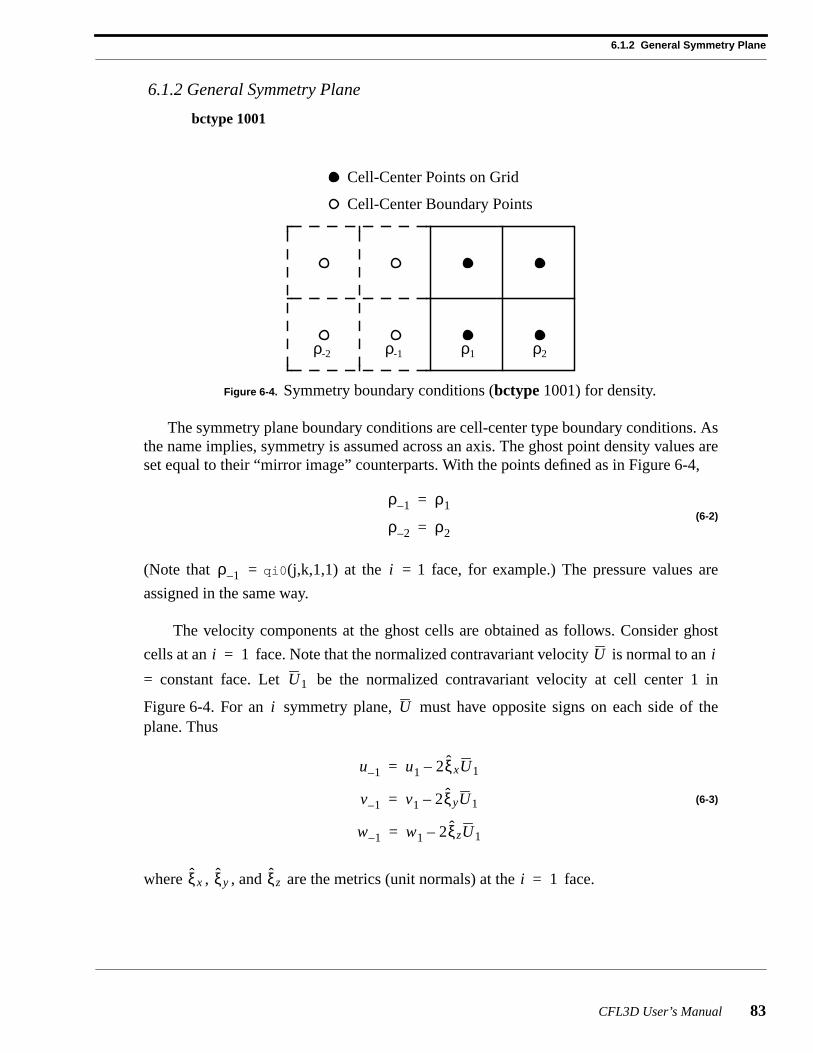
6.1.2 General Symmetry Plane

6.1.2General Symmetry Plane

bctype 1001

The symmetry plane boundary conditions are cell-center type boundary conditions. Asthe name implies, symmetry is assumed across an axis. The ghost point density values areset equal to their “mirror image” counterparts. With the points defined as in Figure6-4,

(6-2)

(Note that = qi0(j,k,1,1) at the = 1 face, for example.) The pressure values are

assigned in the same way.

The velocity components at the ghost cells are obtained as follows. Consider ghost

cells at an face. Note that the normalized contravariant velocity is normal to an

= constant face. Let be the normalized contravariant velocity at cell center 1 in

Figure6-4. For an symmetry plane, must have opposite signs on each side of theplane. Thus

(6-3)

where , , and are the metrics (unit normals) at the face.

Figure 6-4. Symmetry boundary conditions (bctype 1001) for density.



ρ1 ρ2ρ-1ρ-2

ρ 1– ρ1=

ρ 2– ρ2=

ρ 1– i

i 1= U i

U1

i U

u 1– u1 2ξxU1–=

v 1– v1 2ξyU1–=

w 1– w1 2ξzU1–=

ξx ξy ξz i 1=



Since , . The velocity components at ghost cell

center –2 are set in a similar manner using the data at cell center 2. (Note that this is now a“general” symmetry condition, applicable to any plane, not just the plane as in ear-lier versions of the code. Consequently, there is no longer abctype 1006.)

6.1.3Extrapolation

bctype 1002

The extrapolation boundary conditions are cell-center type boundary conditions. Theghost points are extrapolated from the computational domain. Based on the locations of

and depicted in Figure6-4, the extrapolated values would be

(6-4)

The same zeroth order extrapolation is used for the boundary values of the other four flow-field variables.

6.1.4Inflow/Outflow

bctype 1003

The inflow/outflow boundary conditions are cell-face type boundary conditions. In thefar field, the velocity normal to the far boundary (pointingout of the grid) and the speed ofsound are obtained from two locally 1-d Riemann invariants:

(6-5)

where the boundary is considered a surface of constant (in this example) with decreas-

ing corresponding to the interior of the domain and

(6-6)

(6-7)

R– can be evaluated locally from conditions outside the computational domain and R+ canbe determined locally from inside the domain. The normal velocity and speed of sound aredetermined from

ξx( )2

ξy( )2

ξz( )2

+ + 1= U 1– U1=

x z–

ρ1 ρ 1–, ρ 2–

ρ 1– ρ1=

ρ 2– ρ1=

R u2a

γ 1–-----------±≡

ξξ

u Uξt

∇ξ----------–=

Uξx

∇ξ----------u

ξy

∇ξ----------v

ξz

∇ξ----------w

ξt

∇ξ----------+ + +=


6.1.4 Inflo w/Outflo w

(6-8)

The Cartesian velocities are determined by decomposing the normal and tangential veloc-ity vectors:

(6-9)

For inflow, . For outflow, represents the values from the cell inside thedomain adjacent to the boundary.

The sign of the normal velocity determines whether the

condition is at inflow ( ) or outflow ( ). The entropy is deter-

mined using the value from outside the domain for inflow and from inside the domain foroutflow. The entropy and speed of sound are used to determine the density and pressure onthe boundary:

(6-10)

Note that wheni2d = –1, the 1003 boundary condition is augmented by the far-fieldpoint-vortex correction38 (for 2-d, plane only).

u face12--- R

+R

–+( )=

a faceγ 1–

4----------- R

+R

––( )=

u face uref

ξx

∇ξ---------- u face uref–( )+=

v face vref

ξy

∇ξ---------- u face uref–( )+=

w face wref

ξz

∇ξ---------- u face uref–( )+=

ref ∞⇒ ref

U face u face ξt ∇ξ⁄+=

U face 0< U face 0> p ργ⁄

ρ face

a face( )2

γ sface-------------------

1γ 1–-----------

=

p face

ρ face a face( )2

γ--------------------------------=

x z–



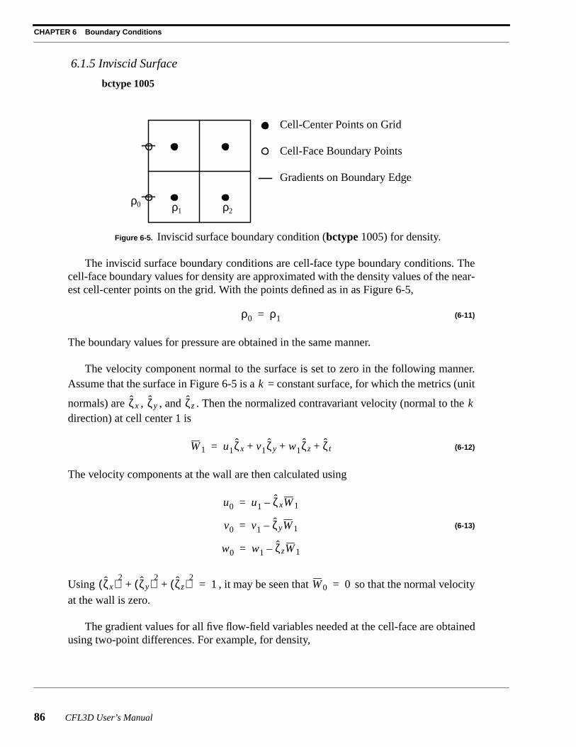
6.1.5Inviscid Surface

bctype 1005

The inviscid surface boundary conditions are cell-face type boundary conditions. Thecell-face boundary values for density are approximated with the density values of the near-est cell-center points on the grid. With the points defined as in as Figure6-5,

(6-11)

The boundary values for pressure are obtained in the same manner.

The velocity component normal to the surface is set to zero in the following manner.Assume that the surface in Figure6-5 is a = constant surface, for which the metrics (unit

normals) are , , and . Then the normalized contravariant velocity (normal to thedirection) at cell center 1 is

(6-12)

The velocity components at the wall are then calculated using

(6-13)

Using , it may be seen that so that the normal velocity

at the wall is zero.

The gradient values for all five flow-field variables needed at the cell-face are obtainedusing two-point differences. For example, for density,

Figure 6-5. Inviscid surface boundary condition (bctype 1005) for density.

ρ1 ρ2ρ0


Cell-Face Boundary Points

Gradients on Boundary Edge

ρ0 ρ1=

k

ζx ζy ζz k

W1 u1ζx v1ζy w1ζz ζt+ + +=

u0 u1 ζxW1–=

v0 v1 ζyW1–=

w0 w1 ζzW1–=

ζx( )2

ζy( )2

ζz( )2

+ + 1= W0 0=


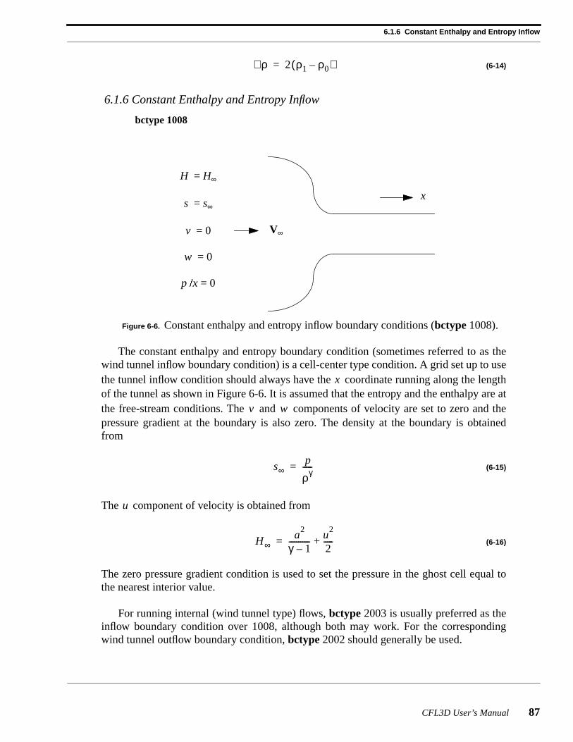
6.1.6 Constant Enthalp y and Entr opy Inflo w

(6-14)

6.1.6Constant Enthalpy and Entropy Inflow

bctype 1008

The constant enthalpy and entropy boundary condition (sometimes referred to as thewind tunnel inflow boundary condition) is a cell-center type condition. A grid set up to usethe tunnel inflow condition should always have the coordinate running along the lengthof the tunnel as shown in Figure6-6. It is assumed that the entropy and the enthalpy are atthe free-stream conditions. The and components of velocity are set to zero and thepressure gradient at the boundary is also zero. The density at the boundary is obtainedfrom

(6-15)

The component of velocity is obtained from

(6-16)

The zero pressure gradient condition is used to set the pressure in the ghost cell equal tothe nearest interior value.

For running internal (wind tunnel type) flows, bctype 2003 is usually preferred as theinflow boundary condition over 1008, although both may work. For the correspondingwind tunnel outflow boundary condition,bctype 2002 should generally be used.

Figure 6-6. Constant enthalpy and entropy inflow boundary conditions (bctype 1008).

ρ∇ 2 ρ1 ρ0–( )=

H = H∞

s = s∞

v = 0

w = 0

p�x = 0

x

V∞

x

v w

s∞p

ργ-----=

u

H∞a

2

γ 1–----------- u

2

2-----+=



6.1.7Singular Axis Using Half-plane Symmetry

bctype 1011

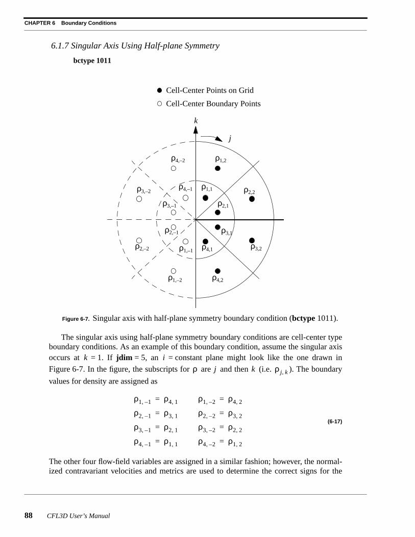
The singular axis using half-plane symmetry boundary conditions are cell-center typeboundary conditions. As an example of this boundary condition, assume the singular axisoccurs at = 1. If jdim = 5, an = constant plane might look like the one drawn in

Figure6-7. In the figure, the subscripts for are and then (i.e. ). The boundary

values for density are assigned as

(6-17)

The other four flow-field variables are assigned in a similar fashion; however, the normal-ized contravariant velocities and metrics are used to determine the correct signs for the

Figure 6-7. Singular axis with half-plane symmetry boundary condition (bctype 1011).



ρ1,1

ρ2,1

ρ2,2

ρ1,2

ρ4,–1

ρ3,–1

ρ3,–2

ρ4,–2

ρ3,1

ρ3,2

ρ4,2

ρ1,–1

ρ2,–1

ρ2,–2

ρ1,–2

j

k

ρ4,1

k i

ρ j k ρ j k,

ρ1 1–, ρ4 1,= ρ1 2–, ρ4 2,=

ρ2 1–, ρ3 1,= ρ2 2–, ρ3 2,=

ρ3 1–, ρ2 1,= ρ3 2–, ρ2 2,=

ρ4 1–, ρ1 1,= ρ4 2–, ρ1 2,=


6.1.8 Singular Axis Using Full Plane , Flux Specified

velocity components in a manner similar to boundary condition type 1001. First note thatby the assumption of half-plane symmetry, the direction cosines on are the same as

apart from the sign; let these metrics be denoted, , and . Then, for

example,

(6-18)

(6-19)

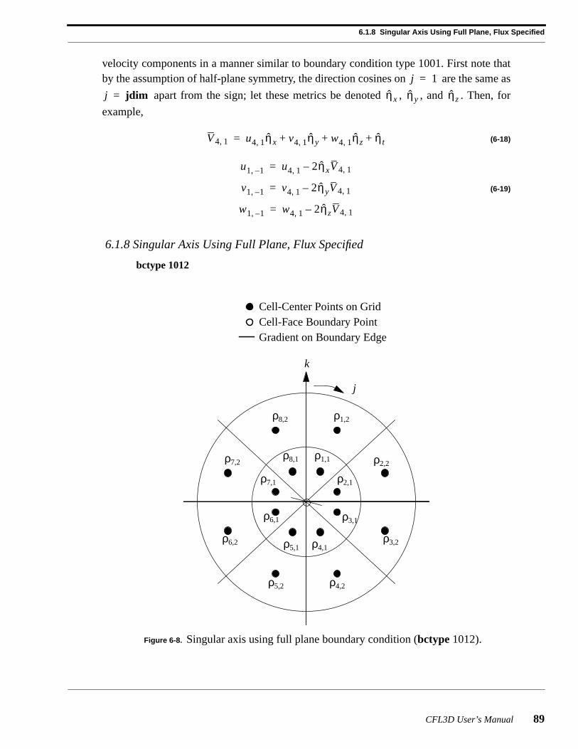
6.1.8Singular Axis Using Full Plane, Flux Specified

bctype 1012

Figure 6-8. Singular axis using full plane boundary condition (bctype 1012).

j 1=

j jdim= ηx ηy ηz

V4 1, u4 1, ηx v4 1, ηy w4 1, ηz ηt+ + +=

u1 1–, u4 1, 2ηxV4 1,–=

v1 1–, v4 1, 2ηyV4 1,–=

w1 1–, w4 1, 2ηzV4 1,–=

Cell-Center Points on GridCell-Face Boundary PointGradient on Boundary Edge

ρ1,1

ρ2,1

ρ2,2

ρ1,2

ρ8,1

ρ7,1

ρ7,2

ρ8,2

ρ3,1

ρ3,2

ρ4,2

ρ5,1

ρ6,1

ρ6,2

ρ5,2

j

k

ρ4,1



The singular axis using full plane boundary conditions are cell-face type boundaryconditions. As an example of this boundary condition, assume the singular axis occurs at

= 1. If jdim = 9, an = constant plane might look like the one drawn in Figure6-8. In

the figure, the subscripts for are and then (i.e. ).

For the cell-face boundary point value of density ( ), an average value of all the val-

ues at = 1 is obtained, i.e.

(6-20)

The flux value is obtained with a two point extrapolation using and :

(6-21)

The boundary values for all five flow-field variables are assigned as described for density.

A known problem exists when using this boundary condition with the Baldwin-Lomaxturbulence model. In such cases, the code employs the “wall” Baldwin-Lomax equationoption rather than the “wake” Baldwin-Lomax equation option at the 1012 boundary.

6.1.9Singular Axis Using Extrapolation (Partial Plane)

bctype 1013

The singular axis using extrapolation boundary conditions are cell-center type bound-ary conditions. The ghost points are extrapolated from the computational domain. Thisboundary condition is used with singular axes for which neither boundary condition type1011 or 1012 is appropriate (quarter planes, for instance). For example, the density bound-ary values would be approximated as

(6-22)

The same first order extrapolation is used for the boundary values of the other flow-fieldvariables.

6.1.10A Word About Singular Metrics

Version 5.0 will automatically detect collapsed grid lines (e.g. singular metrics, cellfaces with zero area) on block boundaries. (Collapsed grid lines in the “interior” of a block

k i

ρ j k ρ j k,

ρ0

k

ρ j 0,

ρ j 1,j 1=

jdim 1–

∑jdim 1–

--------------------------=

ρ1 ρ0

ρ∇( ) j 2 ρ j 1, ρ j 0,–( )=

ρ 1– ρ1=

ρ 2– ρ1=


6.2 Physical Boundary Conditions with Auxiliary Data

are not allowed.) The detection of singular metrics is no longer keyed to the specificationof eitherbctype 1011, 1012, or 1013. While these boundary conditions are still applicable,the new singular metric detection allows any other standard boundary condition that doesnot rely on the grid metrics at the boundary to be used as well. Note that the followingboundary conditions rely on the grid metrics at the boundary and so should not be used ona singular face/face segment: 1001 (symmetry), 1005 (inviscid), 1003 (inflow/outflow),2003 (inflow with specified total conditions) and 2006 (radial equilibrium).

When CFL3D detects singular metrics on a particular block, a message is written tothe main output file (unit 11) indicating the location. It is always a good idea to verify thatany singular block faces/face segments are in fact correctly detected. Metrics are treated assingular if the total area of a face/face segment is less than a parameteratol (set near thetop of subroutinemetric, in modulelbcx.f). In certain cases,atol may need to bechanged (increased in magnitude if faces that are known to be non-singular are flagged assingular and decreased if faces that are known to be singular are not flagged as such, inwhich case the code will give floating point overflow in subroutinemetric).

6.2Physical Boundary Conditions with Auxiliary Data

For the “2000” series of boundary conditions, auxiliary data is required. Therefore,ndata �� wing sections describe the boundary condition types for constant inputdata (ndata > 0). For these conditions, the information in “LT14 - I0 Boundary ConditionSpecification” on page32 through “LT19 - KDIM Boundary Condition Specification” onpage35 is immediately followed by a header line, then a single data line with thendatavalues appropriate for the particular boundary condition. Section6.2.8 describes how touse the same boundary condition types with variable input data.

Input values forbctype (i.e. boundary condition types currently supported) as follows:

bctype boundary condition2002 specified pressure ratio2003 inflow with specified total conditions2004 no-slip wall2005 periodic in space2006 set pressure to satisfy the radial equilibrium equation2007 set all primitive variables2102 pressure ratio specified as a sinusoidal function of time



6.2.1Specified Pressure Ratio

bctype 2002

The specified pressure ratio boundary condition, generally used as the outflow bound-ary condition for internal flows, is a cell-center type boundary condition. A single pressureratio, , is specified on input. The parameterndata must be set to 1 for the input

pressure ratio value to be read. This pressure ratio is used to set both cell-center pressureboundary values ( and ). Extrapolation from inside the computational domain is

used to set the boundary values for , and . See “Extrapolation” on page84. Anexample of the input lines is:

p/pinf0.910

When usingbctype 2002 as the outflow condition for internal (wind tunnel type)flows, the tunnel Mach number and/or mass flow should be monitored andp/pinf adjustedaccordingly to obtain the correct conditions. This is usually an iterative process.

6.2.2Inflow With Specified Total Conditions

bctype 2003

The inflow with specified total conditions boundary condition (sometimes referred toas an “engine inflow” boundary condition because it is often used to specify the conditionsat an inflow face where an engine exhaust is located) is a cell-center type boundary condi-tion. The following five pieces of information are provided on input (ndata = 5): an esti-mated inflow Mach number ( ), the total pressure ratio ( ), the total temperature

ratio ( ), and the flow directions ( and ) in degrees. These values are used as theexternal state in a 1-d characteristic boundary condition. An example of the input lines is:

Mach Pt/Pinf Tt/Tinf Alphae Betae0.300 4.000 1.17555 0.0 0.0

Boundary condition type 2003 is very similar to boundary condition type 1003 in thateither interior or exterior values are chosen, depending on the sign of the characteristics atthe boundary. One difference between them is that, while 1003 uses far-field reference-state levels for the exterior values, 2003 uses the total temperature, pressure, Mach num-ber, and flow angle that are input to determine the reference exterior values. Another dif-ference is the way the density and pressure boundary condition values are determined.Boundary condition type 1003 calculates these values as shown in Equation (6-10).Boundary condition type 2003 first determines a Mach number at the boundary using thevelocities and speed of sound at the boundary (which were calculated through the charac-teristic method):

p p∞⁄

p 1– p 2–

ρ u v, , w

Me pt p∞⁄

Tt T∞⁄ α β


6.2.3 Viscous Surface

(6-23)

It should be noted that the inflow Mach number may end up slightly different from theinput for a converged solution. The pressure and density boundary conditions are then

determined with

(6-24)

The boundary condition velocity components are determined the same way as for bound-ary condition type 1003.

6.2.3Viscous Surface

bctype 2004

The viscous surface boundary conditions are cell-face type boundary conditions. Theno-slip condition ( ) is applied at the surface. Two pieces of auxiliary information

are supplied on input (ndata = 2): the wall temperature ( ) and the mass flow ( ),

where . ( is zero if there is no flow through the wall.) An

example of the input lines is:

Twtype Cq0.95 -0.05

where

Twtype > 0 sets = TwtypeTwtype = 0 sets adiabatic wallTwtype < 0 sets at the stagnation temperatureCq < 0 results in suction (mass flow OUT of the zone)

Cq > 0 results in blowing (mass flow INTO the zone)

Cq = 0 results in no flow through the wall (same as oldbctype 1004)

M2 u

2v

2w

2+ +

a2

-----------------------------=

Me

ppt p∞⁄

γ 1γ 1–

2-----------M

2+

γ γ 1–( )⁄--------------------------------------------------------=

ρ γp

a2

-----=

V 0=

Tw T∞⁄ Cq

Cq ρunormal( ) ρu( )∞⁄= Cq

Tw T∞⁄

Tw



Note that for a dynamic grid,bctype 2004 gives no-slip relative to the moving wall. Toset the wall velocity to zero relative to a non-moving reference frame when the mesh ismoving, use –2004 instead of 2004; this option makes sense only if the grid motion is tan-gential to the surface.

Also note that boundary condition type 2004 supersedes boundary condition types1004and 2004 in previous versions of CFL3D. The main reason for the replacement isthat 1004 relied on global parametersisnd andc2spe to determine whether adiabatic wallor constant-temperature wall conditions were invoked. As a consequence, all 1004 seg-ments had to be the same. Now, with 2004 (along with its additional data fieldTwtype),every no-slip wall segment can be set with different wall temperature conditions, ifdesired. Boundary condition type 2004 also allows for mass flow through the wall (suctionor blowing) through the second additional data fieldCq.

The no-slip wall boundary condition is implemented as follows:

• The nondimensional pressure on the body is determined through linear extrapola-

tion:

(6-25)

But if , then . Here the indices 1 and 2 indicate the first and second cell-

center values away from the wall, respectively.

• The nondimensional square of the speed of sound, variablec2, at the wall is next deter-

mined. (Note thatc2 = .)

If Twtype > 0,c2 = Twtype.

If Twtype < 0,c2 = .

If Twtype = 0,c2 = .

• The surface velocities are then determined as

(6-26)

pb

pb p1 p2 p1–( ) 2⁄–=

pb 0< pb p1=

aw a∞⁄( )2Tw T∞⁄=

1γ 1–

2----------- M∞( )2

+

a1

a∞------

21

γ 1–2

----------- M1( )2+

uw M∞Cq

ξx

∇ξ---------- c2( )

γ pb----------- umesh+=

vw M∞Cq

ξy

∇ξ---------- c2( )

γ pb----------- vmesh+=

ww M∞Cq

ξz

∇ξ---------- c2( )

γ pb----------- wmesh+=


6.2.4 Periodic (In Space)

where , , and are the velocity components of the mesh (they equal 0

if the grid/body is not in motion).

• Since 2004 is a cell-face boundary condition type (i.e. the boundary conditions andtheir gradient are applied at the cell face rather than in ghost cells),

(6-27)

The gradients at the wall for all the primitive variables are determined via, etc.

Note thatsmin is computed from viscous wallsonly. If a wall is inviscid, then as far assmin is concerned, it is invisible. This is important to remember when viscous boundaryconditions are turned on after running a case inviscidly for some time sincesmin maynever have been computed!

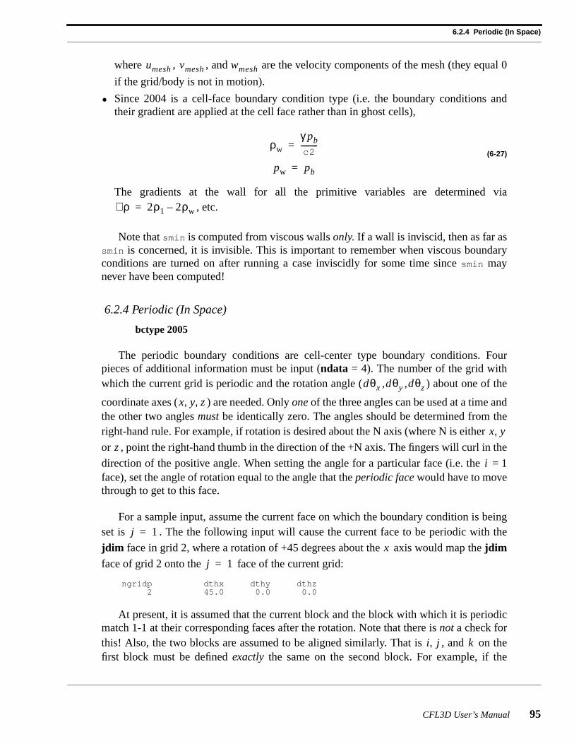
6.2.4Periodic (In Space)

bctype 2005

The periodic boundary conditions are cell-center type boundary conditions. Fourpieces of additional information must be input (ndata = 4). The number of the grid withwhich the current grid is periodic and the rotation angle (, , ) about one of the

coordinate axes ( ) are needed. Onlyoneof the three angles can be used at a time andthe other two anglesmust be identically zero. The angles should be determined from theright-hand rule. For example, if rotation is desired about the N axis (where N is either

or , point the right-hand thumb in the direction of the +N axis. The fingers will curl in the

direction of the positive angle. When setting the angle for a particular face (i.e. the = 1face), set the angle of rotation equal to the angle that theperiodicface would have to movethrough to get to this face.

For a sample input, assume the current face on which the boundary condition is beingset is . The the following input will cause the current face to be periodic with the

jdim face in grid 2, where a rotation of +45 degrees about the axis would map thejdimface of grid 2 onto the face of the current grid:

ngridp dthx dthy dthz2 45.0 0.0 0.0

At present, it is assumed that the current block and the block with which it is periodicmatch 1-1 at their corresponding faces after the rotation. Note that there isnot a check forthis! Also, the two blocks are assumed to be aligned similarly. That is , and on thefirst block must be definedexactly the same on the second block. For example, if the

umesh vmesh wmesh

ρw

γ pb

c2---------=

pw pb=

ρ∇ 2ρ1 2ρw–=

dθx dθy dθz

x y z, ,

x y,z

i

j 1=

x

j 1=

i j, k



= kdim face of the current block has the periodic boundary condition applied to it, it is

implicitly assumed that it is periodic with the face of the specified second block

and and run in the exact same directions on both blocks. Note that this means that twoof the dimensions (idim andjdim in the example) must be the same on both blocks.

The periodic boundary condition also works for a grid with one cell (two grid planes)in the periodic direction if the grid is set to be periodic with itself. Note, however, that if aparticular block is periodic with adifferent block, then neither block should be only onecell wide in the periodic direction.

In addition, the periodic boundary condition may be used for linear displacement, pro-vided the rotation angles are set to zero. Alternatively, the 1-1 block connection can beused (linear displacement only!). The 1-1 internal check will flag geometric mismatches,which should be equal to the desired linear periodic displacement. This is a good check ofthe input which is not available with boundary condition type 2005.

Boundary condition type 2005 is a limited-use periodic (in space) boundary condition.For example, if one is solving for flow through a duct and it is known that the solution isperiodic over 90 degrees (i.e. the solution is identical in each of the four quadrants of theduct), then a solution need only be obtained on a grid spanning 90 degrees, with periodicboundary conditions applied at the two edges.

For an illustration of how this boundary condition works, consider Figure6-9. Thisexample is for flow through a 90 degree wedge (the flow direction is in the third dimen-sion, out of the page). The flow is periodic over 90 degrees, so periodic boundary condi-tions are applied at the and faces.

Figure 6-9. Periodic boundary condition (bctype 2005) example.

k

k 1=

i j

j 0= j jdim=

jdim–2

1 2

qj0(1)qj0(2)

qj0(3)

qj0(4)

jdim–1

z

y


6.2.5 Radial Pressure Equilibrium

For density and pressure, boundary condition type 2005 sets:

(6-28)

The boundary conditions for the velocity components , , and are assigned simi-

larly, except that they are first rotated through the periodic angle, in this case. Forexample,

(6-29)

For an example of how this boundary condition can be used for linear displacement,see the 2-d vibrating plate sample test case in Section9.1.6 on page177.

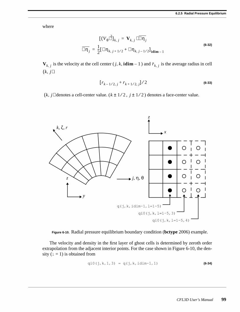
6.2.5Radial Pressure Equilibrium

bctype 2006

Boundary condition type 2006 is a cell-center type boundary condition. Radial pres-sure equilibrium is used as a downstream boundary condition when it is desired to specifya pressure, but a large swirling component is present in the flow. Typically, this boundarycondition would be used in turbomachinery applications in which a swirling flow is estab-lished by a rotor that is not corrected by the presence of stators or exit guide vanes.

Four additional pieces of information are needed for this boundary condition type(ndata = 4). The grid number (ngridc) of the gridfrom which the integration of pressureis to be continued is specified. If the integration in this grid is not continued from anothergrid, input 0. A value for is input. Ifngridc = 0, this value will be the starting value

for the integration. Ifngridc 0, then the pressure value from the connecting point in gridngridc is used as the starting value for the integration in the current block. The direction inwhich integration is to proceed is specified with the parameterintdir. It may have an abso-lute value of 1, 2, or 3 for integration in the , or directions, respectively. The sign ofintdir indicates whether the integration proceeds in the increasing (positive) or decreasing(negative) coordinate direction. Theintdir direction must be the radial direction. Thefourth piece of information needed is the physical direction along which the radial axislies, denoted with the parameteraxcoord. It may have the values of +1, +2, or +3 for aradial axis aligned with the , or axes. The input lines for this boundary conditiontype would look like:

ngridc P/Pinf intdir axcoord

qj0(1) q(jdim-1)=

qj0(2) q(jdim-2)=

qj0(3) q(1)=

qj0(4) q(2)=

u v w

90°

u1 BC, qj0 k i 2 1, , ,( ) q j k i 2, , ,( ) (unchanged)= =

v1 BC, qj0 k i 3 1, , ,( ) q j k i 3, , ,( ) θp q j k i 4, , ,( ) θpsin–cos= =

w1 BC, qj0 k i 4 1, , ,( ) q j k i 3, , ,( ) θp q j k i 4, , ,( ) θpcos+sin= =

p p∞⁄

i j, k

x y, z



0 0.9 +3 1

The radial equilibrium condition requires that the pressure satisfy

(6-30)

where is the circumferential velocity component and is the radius. The pressure

ratio, , is set at either the bottom or the top of the block face and then the radial

equilibrium equation is integrated in either the increasing or decreasing radial direction togive the pressure at all other radii. The trapezoidal rule is used to perform the integration.The other flow-field variables ( ) are extrapolated from inside the computationaldomain. See “Extrapolation” on page84.

This boundary condition assumes that one coordinate direction on the block face isessentially radial and the other is essentially circumferential and that the integration isbeing carried out in the radial direction. Since there is no way to verify this in the code,caremust be exercised when using this boundary condition to insure that this and the fol-lowing restrictions are met. Continuation of the radial equilibrium condition through blockboundaries is restricted to blocks that have thesame orientation. For example, if the equi-librium condition is to be continued through a boundary from an adjacent block, then

and must run in the same direction in both blocks. This also implies that the boundary

must be = 1 in one block and = kdim in the second (i.e. the boundary can not be

= 1 in both blocks). Also, the segment must run the entire length of the block face in thedirection in which the integration is being carried out. For example, if the integration isbeing carried out in the direction, thenksta must be set to 1 andkend must be set tokdim. This restriction applies only if the integration is being continued from anotherblock.

Consider a case in which boundary condition 2006 is to be applied at an = idim face,

with = constant radial lines (i.e. lines of constant angle) and = constant circumfer-

ential lines (i.e. lines of constant radius). Assume the block face lies in an = constantplane, as shown in Figure6-10.

Assuming integration in the + direction (intdir = 3), the pressure (l = 5) in the firstplane of ghost cells is obtained from

(6-31)

dpdr------ ρ

Vθ( )2

r--------------=

Vθ r

p p∞⁄

ρ u v w, , ,

k i

j k

k k

k

k

i

j θ k

x

k

qi0(j,1,5,3)p

p∞------

p∞=

qi0(j,k,5,3) pk j, pk 1 j,–

ρk j, Vθ( )2[ ]k j,r k j,

-----------------------------------∆r k j,+= = k 2 kdim 1–,=


6.2.5 Radial Pressure Equilibrium

where

(6-32)

is the velocity at the cell center ( ) and is the average radius in cell

:

(6-33)

denotes a cell-center value. ( , ) denotes a face-center value.

The velocity and density in the first layer of ghost cells is determined by zeroth orderextrapolation from the adjacent interior points. For the case shown in Figure6-10, the den-sity (l = 1) is obtained from

qi0(j,k,1,3) = q(j,k,idim-1,1) (6-34)

Figure 6-10. Radial pressure equilibrium boundary condition (bctype 2006) example.

Vθ( )2[ ]k j, Vk j, ∇η j⋅=

∇η j12--- ∇ηk j 1 2⁄+, ∇ηk j 1 2⁄–,+[ ]idim 1–=

Vk j, j k idim 1–, , r k j,

k j,( )

r k 1 2⁄ j,– r k 1 2⁄ j,++[ ] 2⁄

k j,( ) k 1 2⁄± j 1 2⁄±

q(j,k,idim-1,l=1-5)

qi0(j,k,l=1-5,3)

qi0(j,k,l=1-5,4)

z

xk, ζ, r

j, η, θz

y



All flow quantities in the second layer of ghost cells are obtained by zeroth orderextrapolation from the first layer of ghost cells:

qi0(j,k,l=1-5,4) = qi0(j,k,l=1-5,3) (6-35)

6.2.6Specify All Primitive Variables

bctype 2007

Boundary condition type 2007 is a cell-center type boundary condition. It involves set-ting the boundary conditions with the five (ndata = 5) primitive variables, using standard

CFL3D normalizations: , , , , and . An example of

the input lines is:

rho/rho_inf u/a_inf v/a_inf w/a_inf p/(rho_inf*a_inf**2)1.0 0.3 0.0 0.0 0.71

Note that the input pressure isnot but rather . Also note that the turbu-

lence quantities arenot currently allowed to be specified in the same way as theq’s.Instead, they are extrapolated from the interior whenbctype 2007 is employed.

6.2.7Specified Pressure Ratio As Sinusoidal Time Function

bctype 2102

The specified pressure ratio as a sinusoidal function of time boundary conditions arecell-center type boundary conditions. The pressure ratio, , is specified as a sinusoi-

dal function of time. The other flow-field variables ( ) are extrapolated frominside the computational domain. Three pieces of additional information are specified oninput (ndata = 4): the desired baseline (steady) pressure ratio ( ), the amplitude of

the pressure oscillation ( ), the reduced frequency of the pressure oscillation (),

and the “grid equivalent” of the dimensional reference length used to define the reducedfrequency ( ). The pressure will vary as

(6-36)

The reduced frequency is non-dimensionalized by

(6-37)

where is the frequency in cycles per second, is a characteristic length and is thefree-stream speed of sound. (Note that this definition of reduced frequency differs from

ρ ρ∞⁄ u a∞⁄ v a∞⁄ w a∞⁄ p ρ∞ a∞( )2[ ]⁄

p p∞⁄ p γ p∞( )⁄

p p∞⁄

ρ u v w, , ,

p p∞⁄

∆ p p∞⁄ kr

Lref

γpp

p∞------

∆ pp∞------- 2πkr t( )sin+=

krf La∞-------=

f L a∞


6.2.8 Variable Data for the 2000 Series

the “standard” definition .) An example of the lines in the input file for this

boundary condition is:

p/pinf deltap/pinf rfreqp lref0.910 0.001 175.93 1.0

6.2.8Variable Data for the 2000 Series

To use this option, setndata = –(the ndata used for the constant data value(s) asdescribed above). Then, instead of the line containing the constant data value(s), substitutea line with the name (up to 60 characters) of a formatted file that has the appropriate arrayof data values. The data file will then be read with the following format:

read(iunit,*) header/titleread(iunit,*) mdim,ndim,np mdim,ndim = cell-center dimensions of segment

np = number of planes of ghost cell dataread(iunit,*) nvalues number of data values;nvalues = abs(ndata)read(iunit,*)((((bcdata(m,n,ip,l),m=1,mdim),n=1,ndim),ip=1,np),

l=1,nvalues)

The roles ofm,n vary depending on which face the segment is located:

Note that zeroes arenot acceptable formdim or ndim. Use the actual values of jdim-1,kdim-1, and/oridim-1 for the full face. Only boundary condition type 2007 can make useof two planes of data. For all other boundary conditions, setnp = 1.

6.3Block Interface Boundary Conditions

For all the types of block interface boundary conditions, setbctype = 0. If bctype 0,but block interface boundary conditions are set, the block interface boundary conditionswill supersede. All block interface boundary conditions (one-to-one, patched, and overset)are cell-center type boundary conditions.

on the = 1 and the = idim faces wheremdim = jend–jsta andndim = kend–kstaon the = 1 and the = jdim faces wheremdim = kend–ksta andndim = iend–istaon the = 1 and the = kdim faces wheremdim = jend–jsta andndim = iend–ista

kr f L V ∞⁄=

m n, j k,→ i i

m n, k i,→ j j

m n, j i,→ k k



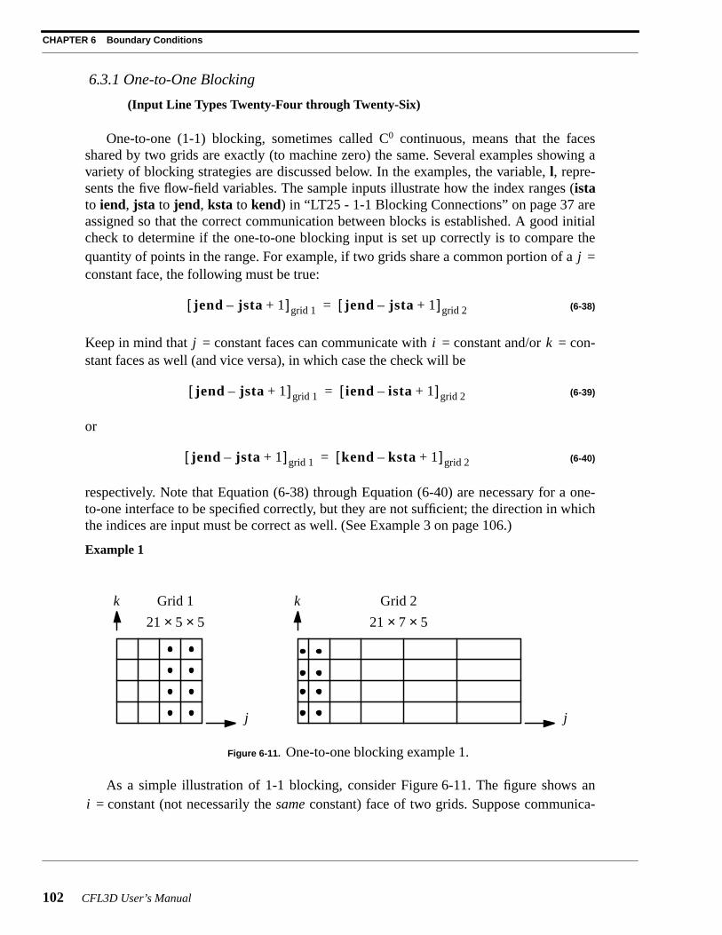
6.3.1One-to-One Blocking

(Input Line Types Twenty-Four through Twenty-Six)

One-to-one (1-1) blocking, sometimes called C0 continuous, means that the facesshared by two grids are exactly (to machine zero) the same. Several examples showing avariety of blocking strategies are discussed below. In the examples, the variable,l, repre-sents the five flow-field variables. The sample inputs illustrate how the index ranges (istato iend, jsta to jend, ksta to kend) in “LT25 - 1-1 Blocking Connections” on page37 areassigned so that the correct communication between blocks is established. A good initialcheck to determine if the one-to-one blocking input is set up correctly is to compare thequantity of points in the range. For example, if two grids share a common portion of a =constant face, the following must be true:

(6-38)

Keep in mind that = constant faces can communicate with = constant and/or = con-stant faces as well (and vice versa), in which case the check will be

(6-39)

or

(6-40)

respectively. Note that Equation (6-38) through Equation (6-40) are necessary for a one-to-one interface to be specified correctly, but they are not sufficient; the direction in whichthe indices are input must be correct as well. (See Example 3 on page106.)

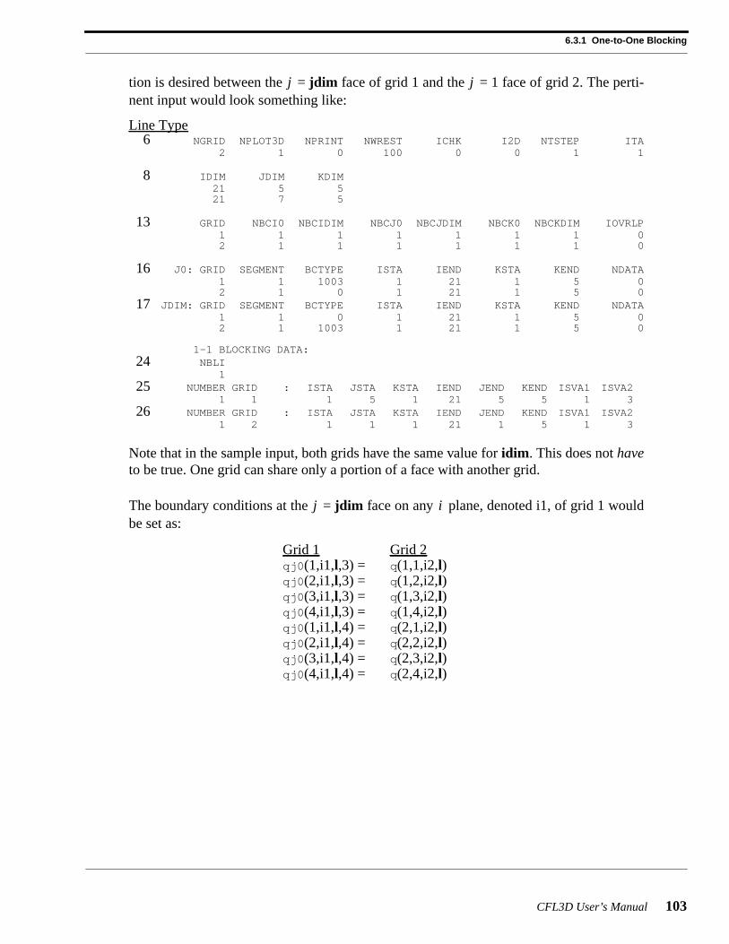
Example 1

As a simple illustration of 1-1 blocking, consider Figure6-11. The figure shows an= constant (not necessarily thesame constant) face of two grids. Suppose communica-

Figure 6-11. One-to-one blocking example 1.

j

jend jsta– 1+[ ]grid 1 jend jsta– 1+[ ]grid 2=

j i k

jend jsta– 1+[ ]grid 1 iend ista– 1+[ ]grid 2=

jend jsta– 1+[ ]grid 1 kend ksta– 1+[ ]grid 2=

k k

j j

Grid 1 Grid 2

21 × 5 × 5 21 × 7 × 5

i


6.3.1 One-to-One Blocking

tion is desired between the = jdim face of grid 1 and the = 1 face of grid 2. The perti-nent input would look something like:

Line Type6 NGRID NPLOT3D NPRINT NWREST ICHK I2D NTSTEP ITA

2 1 0 100 0 0 1 1

8 IDIM JDIM KDIM21 5 521 7 5

13 GRID NBCI0 NBCIDIM NBCJ0 NBCJDIM NBCK0 NBCKDIM IOVRLP1 1 1 1 1 1 1 02 1 1 1 1 1 1 0

16 J0: GRID SEGMENT BCTYPE ISTA IEND KSTA KEND NDATA1 1 1003 1 21 1 5 02 1 0 1 21 1 5 0

17 JDIM: GRID SEGMENT BCTYPE ISTA IEND KSTA KEND NDATA1 1 0 1 21 1 5 02 1 1003 1 21 1 5 0

1-1 BLOCKING DATA:24 NBLI

125 NUMBER GRID : ISTA JSTA KSTA IEND JEND KEND ISVA1 ISVA2

1 1 1 5 1 21 5 5 1 326 NUMBER GRID : ISTA JSTA KSTA IEND JEND KEND ISVA1 ISVA2

1 2 1 1 1 21 1 5 1 3

Note that in the sample input, both grids have the same value for idim. This does not haveto be true. One grid can share only a portion of a face with another grid.

The boundary conditions at the = jdim face on any plane, denoted i1, of grid 1 wouldbe set as:

Grid 1 Grid 2qj0(1,i1,l,3) = q(1,1,i2,l)qj0(2,i1,l,3) = q(1,2,i2,l)qj0(3,i1,l,3) = q(1,3,i2,l)qj0(4,i1,l,3) = q(1,4,i2,l)qj0(1,i1,l,4) = q(2,1,i2,l)qj0(2,i1,l,4) = q(2,2,i2,l)qj0(3,i1,l,4) = q(2,3,i2,l)qj0(4,i1,l,4) = q(2,4,i2,l)

j j

j i



The boundary conditions at the= 1 face on any plane, denoted i2, of grid 2 would beset as:

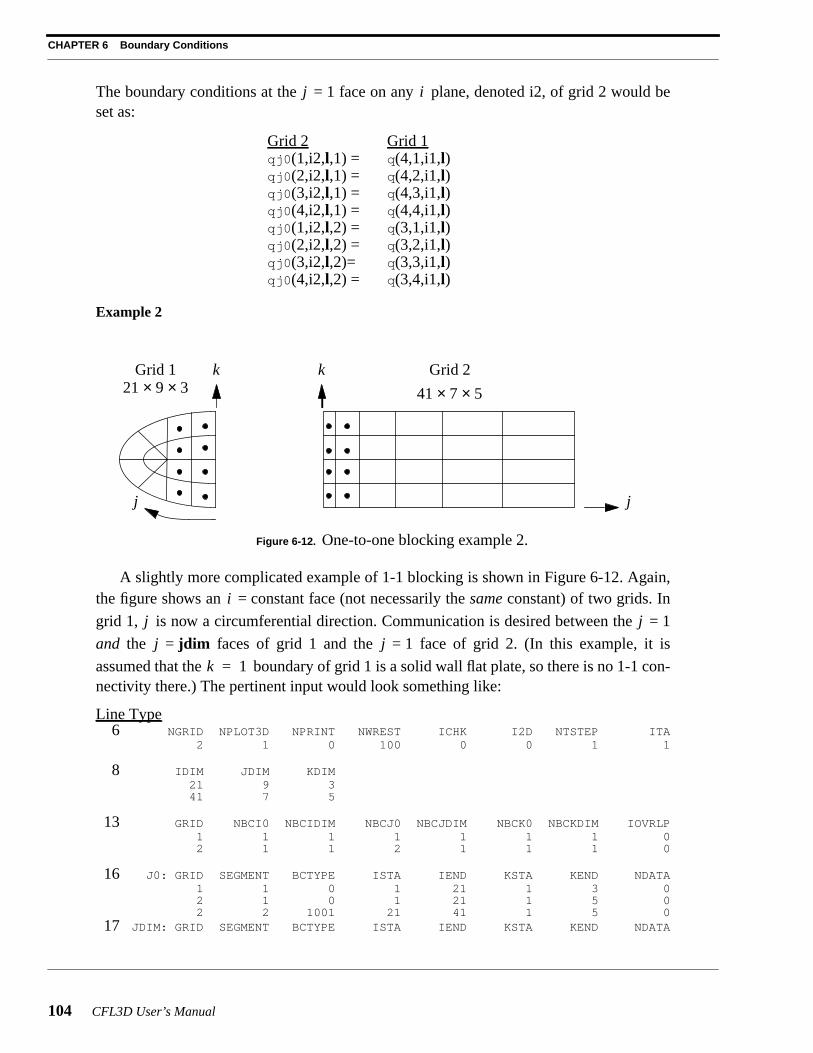
Example 2

A slightly more complicated example of 1-1 blocking is shown in Figure6-12. Again,the figure shows an = constant face (not necessarily thesame constant) of two grids. In

grid 1, is now a circumferential direction. Communication is desired between the= 1

and the = jdim faces of grid 1 and the = 1 face of grid 2. (In this example, it is

assumed that the boundary of grid 1 is a solid wall flat plate, so there is no 1-1 con-nectivity there.) The pertinent input would look something like:


2 1 0 100 0 0 1 1



16 J0: GRID SEGMENT BCTYPE ISTA IEND KSTA KEND NDATA1 1 0 1 21 1 3 02 1 0 1 21 1 5 02 2 1001 21 41 1 5 0

17 JDIM: GRID SEGMENT BCTYPE ISTA IEND KSTA KEND NDATA

Grid 2 Grid 1qj0(1,i2,l,1) = q(4,1,i1,l)qj0(2,i2,l,1) = q(4,2,i1,l)qj0(3,i2,l,1) = q(4,3,i1,l)qj0(4,i2,l,1) = q(4,4,i1,l)qj0(1,i2,l,2) = q(3,1,i1,l)qj0(2,i2,l,2) = q(3,2,i1,l)qj0(3,i2,l,2)= q(3,3,i1,l)qj0(4,i2,l,2) = q(3,4,i1,l)


j i

k

j j

Grid 1 Grid 2 k21 × 9 × 3 41 × 7 × 5

i

j j

j j

k 1=



1 1 0 1 21 1 3 02 1 1003 1 41 1 5 0



1 1 1 1 1 21 1 3 1 32 1 1 9 1 21 9 3 1 3

26 NUMBER GRID : ISTA JSTA KSTA IEND JEND KEND ISVA1 ISVA21 2 1 1 3 21 1 1 1 32 2 1 1 3 21 1 5 1 3

Note how ranges on grid 2 to coincide with the appropriate points on the = 1 and

= jdim faces of grid 1. This sample input also shows how grid 1 can share only a portion

of the = 1 face of grid 2 in the direction.

The boundary conditions at the = 1 face on any plane, denoted i1, of grid 1 would beset as:

The boundary conditions at the = jdim face for the i1 plane of grid 1 would be set as:

The boundary conditions at the = 1 face on any plane, denoted i2, of grid 2 would beset as:

Grid 1 Grid 2qj0(1,i1,l,1) = q(1,2,i2,l)qj0(2,i1,l,1) = q(1,1,i2,l)qj0(1,i1,l,2) = q(2,2,i2,l)qj0(2,i1,l,2) = q(2,1,i2,l)

Grid 1 Grid 2qj0(1,i1,l,3) = q(1,3,i2,l)qj0(2,i1,l,3) = q(1,4,i2,l)qj0(1,i1,l,4) = q(2,3,i2,l)qj0(2,i1,l,4) = q(2,4,i2,l)

Grid 2 Grid 1qj0(1,i2,l,1) = q(1,2,i1,l)qj0(2,i2,l,1) = q(1,1,i1,l)qj0(3,i2,l,1) = q(8,1,i1,l)qj0(4,i2,l,1) = q(8,2,i1,l)qj0(1,i2,l,2) = q(2,2,i1,l)qj0(2,i2,l,2) = q(2,1,i1,l)qj0(3,i2,l,2) = q(7,1,i1,l)qj0(4,i2,l,2) = q(7,2,i1,l)

k k j

j

j i

j i

j

j i



Example 3

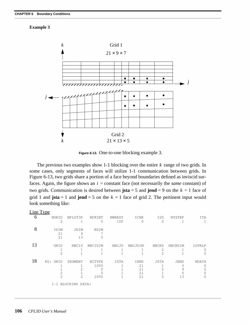
The previous two examples show 1-1 blocking over the entire range of two grids. Insome cases, only segments of faces will utilize 1-1 communication between grids. InFigure6-13, two grids share a portion of a face beyond boundaries defined as inviscid sur-faces. Again, the figure shows an = constant face (not necessarily thesame constant) of

two grids. Communication is desired betweenjsta = 5 andjend = 9 on the = 1 face of

grid 1 andjsta = 1 andjend = 5 on the = 1 face of grid 2. The pertinent input wouldlook something like:


2 1 0 100 0 0 1 1



18 K0: GRID SEGMENT BCTYPE ISTA IEND JSTA JEND NDATA1 1 1005 1 21 1 5 01 2 0 1 21 5 9 02 1 0 1 21 1 5 02 2 1005 1 21 5 13 0

1-1 BLOCKING DATA:


j

j

k

k

Grid 1

Grid 2

21 × 9 × 7

21 × 13× 5

k

i

k

k



24 NBLI1

25 NUMBER GRID : ISTA JSTA KSTA IEND JEND KEND ISVA1 ISVA21 1 1 5 1 21 9 1 1 2

26 NUMBER GRID : ISTA JSTA KSTA IEND JEND KEND ISVA1 ISVA21 2 1 5 1 21 1 1 1 2

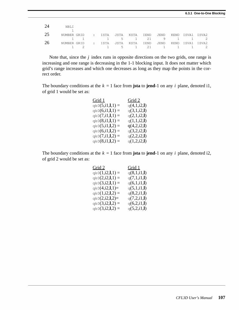
Note that, since the index runs in opposite directions on the two grids, one range isincreasing and one range is decreasing in the 1-1 blocking input. It does not matter whichgrid’s range increases and which one decreases as long as they map the points in the cor-rect order.

The boundary conditions at the= 1 face fromjsta to jend-1 on any plane, denoted i1,of grid 1 would be set as:

The boundary conditions at the= 1 face fromjsta to jend-1 on any plane, denoted i2,of grid 2 would be set as:

Grid 1 Grid 2qk0(5,i1,l,1) = q(4,1,i2,l)qk0(6,i1,l,1) = q(3,1,i2,l)qk0(7,i1,l,1) = q(2,1,i2,l)qk0(8,i1,l,1) = q(1,1,i2,l)qk0(5,i1,l,2) = q(4,2,i2,l)qk0(6,i1,l,2) = q(3,2,i2,l)qk0(7,i1,l,2) = q(2,2,i2,l)qk0(8,i1,l,2) = q(1,2,i2,l)

Grid 2 Grid 1qk0(1,i2,l,1) = q(8,1,i1,l)qk0(2,i2,l,1) = q(7,1,i1,l)qk0(3,i2,l,1) = q(6,1,i1,l)qk0(4,i2,l,1)= q(5,1,i1,l)qk0(1,i2,l,2) = q(8,2,i1,l)qk0(2,i2,l,2)= q(7,2,i1,l)qk0(3,i2,l,2) = q(6,2,i1,l)qk0(3,i2,l,2) = q(5,2,i1,l)

j

k i

k i



Example 4

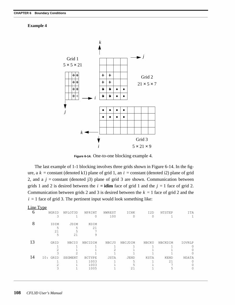
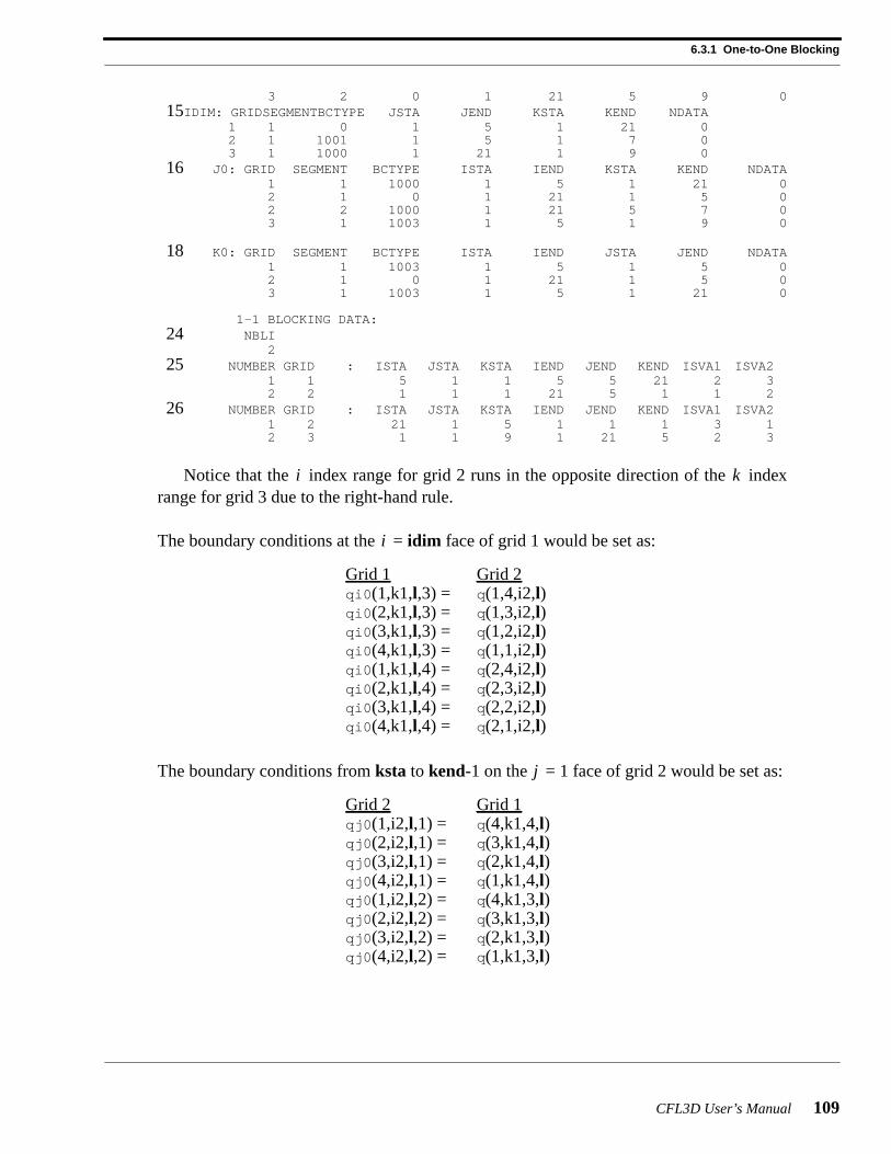
The last example of 1-1 blocking involves three grids shown in Figure6-14. In the fig-ure, a = constant (denoted k1) plane of grid 1, an= constant (denoted i2) plane of grid

2, and a = constant (denoted j3) plane of grid 3 are shown. Communication between

grids 1 and 2 is desired between the= idim face of grid 1 and the = 1 face of grid 2.

Communication between grids 2 and 3 is desired between the = 1 face of grid 2 and the

= 1 face of grid 3. The pertinent input would look something like:


3 1 0 100 0 0 1 1

8 IDIM JDIM KDIM5 5 21

21 5 75 21 9

13 GRID NBCI0 NBCIDIM NBCJ0 NBCJDIM NBCK0 NBCKDIM IOVRLP1 1 1 1 1 1 1 02 1 1 2 1 1 1 03 2 1 1 1 1 1 0

14 I0: GRID SEGMENT BCTYPE JSTA JEND KSTA KEND NDATA1 1 1003 1 5 1 21 02 1 1003 1 5 1 7 03 1 1005 1 21 1 5 0


i

j

k

j

i

k

Grid 1

Grid 2

Grid 3

21 × 5 × 7

5 × 21× 9

5 × 5 × 21

k i

j

i j

k

i



3 2 0 1 21 5 9 015IDIM: GRIDSEGMENTBCTYPE JSTA JEND KSTA KEND NDATA

1 1 0 1 5 1 21 02 1 1001 1 5 1 7 03 1 1000 1 21 1 9 0

16 J0: GRID SEGMENT BCTYPE ISTA IEND KSTA KEND NDATA1 1 1000 1 5 1 21 02 1 0 1 21 1 5 02 2 1000 1 21 5 7 03 1 1003 1 5 1 9 0

18 K0: GRID SEGMENT BCTYPE ISTA IEND JSTA JEND NDATA1 1 1003 1 5 1 5 02 1 0 1 21 1 5 03 1 1003 1 5 1 21 0



1 1 5 1 1 5 5 21 2 32 2 1 1 1 21 5 1 1 2

26 NUMBER GRID : ISTA JSTA KSTA IEND JEND KEND ISVA1 ISVA21 2 21 1 5 1 1 1 3 12 3 1 1 9 1 21 5 2 3

Notice that the index range for grid 2 runs in the opposite direction of the indexrange for grid 3 due to the right-hand rule.

The boundary conditions at the = idim face of grid 1 would be set as:

The boundary conditions from ksta to kend-1 on the = 1 face of grid 2 would be set as:

Grid 1 Grid 2qi0(1,k1,l,3) = q(1,4,i2,l)qi0(2,k1,l,3) = q(1,3,i2,l)qi0(3,k1,l,3) = q(1,2,i2,l)qi0(4,k1,l,3) = q(1,1,i2,l)qi0(1,k1,l,4) = q(2,4,i2,l)qi0(2,k1,l,4) = q(2,3,i2,l)qi0(3,k1,l,4) = q(2,2,i2,l)qi0(4,k1,l,4) = q(2,1,i2,l)

Grid 2 Grid 1qj0(1,i2,l,1) = q(4,k1,4,l)qj0(2,i2,l,1) = q(3,k1,4,l)qj0(3,i2,l,1) = q(2,k1,4,l)qj0(4,i2,l,1) = q(1,k1,4,l)qj0(1,i2,l,2) = q(4,k1,3,l)qj0(2,i2,l,2) = q(3,k1,3,l)qj0(3,i2,l,2) = q(2,k1,3,l)qj0(4,i2,l,2) = q(1,k1,3,l)

i k

i

j



The boundary conditions at the = 1 face of grid 2 would be set as:

The boundary conditions from ksta to kend-1 on the = 1 face of grid 3 would be set as:

Grid 2 Grid 3qk0(1,i2,l,1) = q(j3,8,1,l)qk0(2,i2,l,1) = q(j3,7,1,l)qk0(3,i2,l,1) = q(j3,6,1,l)qk0(4,i2,l,1) = q(j3,5,1,l)qk0(1,i2,l,2) = q(j3,8,2,l)qk0(2,i2,l,2) = q(j3,7,2,l)qk0(3,i2,l,2) = q(j3,6,2,l)qk0(4,i2,l,2) = q(j3,5,2,l)

Grid 3 Grid 2qi0(j3,5,l,1) = q(4,1,i2,l)qi0(j3,6,l,1) = q(3,1,i2,l)qi0(j3,7,l,1) = q(2,1,i2,l)qi0(j3,8,l,1) = q(1,1,i2,l)qi0(j3,5,l,2) = q(4,2,i2,l)qi0(j3,6,l,2) = q(3,2,i2,l)qi0(j3,7,l,2) = q(2,2,i2,l)qi0(j3,8,l,2) = q(1,2,i2,l)

k

i


6.3.2 Patched-Grid Interpolation

6.3.2Patched-Grid Interpolation

(Input Line Type Twenty-Seven)

6.3.2.1General Information

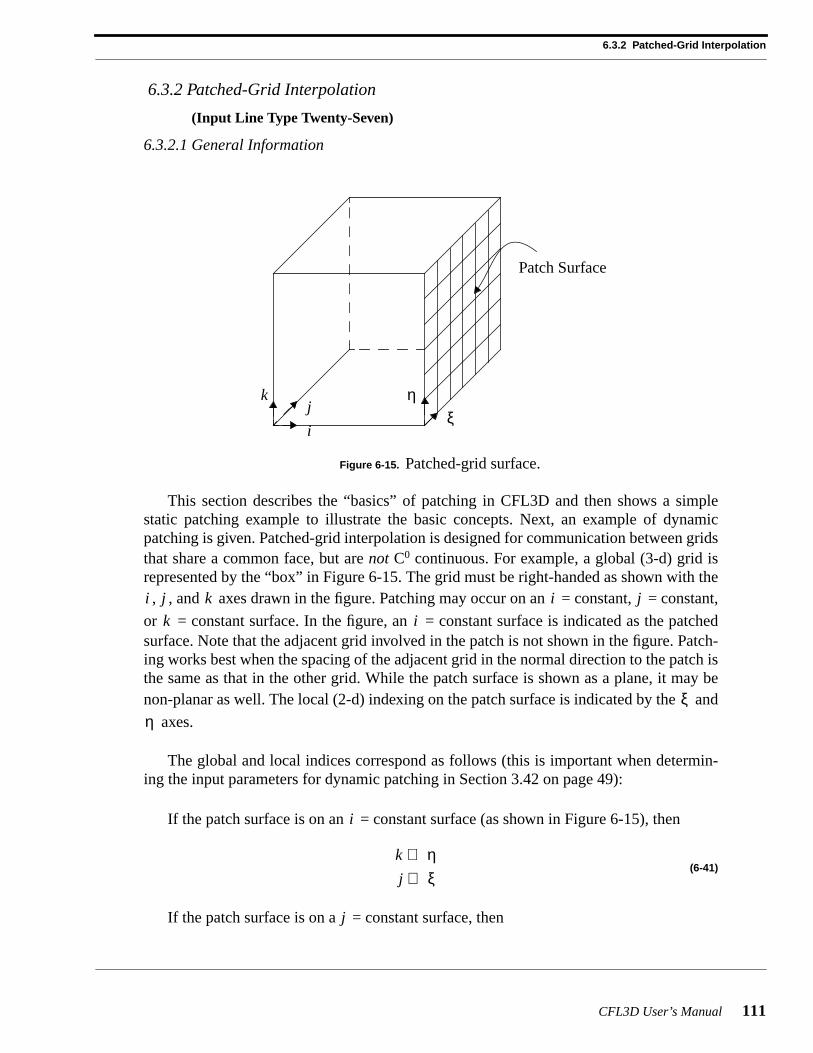
This section describes the “basics” of patching in CFL3D and then shows a simplestatic patching example to illustrate the basic concepts. Next, an example of dynamicpatching is given. Patched-grid interpolation is designed for communication between gridsthat share a common face, but arenot C0 continuous. For example, a global (3-d) grid isrepresented by the “box” in Figure6-15. The grid must be right-handed as shown with the, , and axes drawn in the figure. Patching may occur on an = constant, = constant,

or = constant surface. In the figure, an = constant surface is indicated as the patchedsurface. Note that the adjacent grid involved in the patch is not shown in the figure. Patch-ing works best when the spacing of the adjacent grid in the normal direction to the patch isthe same as that in the other grid. While the patch surface is shown as a plane, it may benon-planar as well. The local (2-d) indexing on the patch surface is indicated by the and

axes.

The global and local indices correspond as follows (this is important when determin-ing the input parameters for dynamic patching in Section3.42 on page49):

If the patch surface is on an = constant surface (as shown in Figure6-15), then

(6-41)

If the patch surface is on a = constant surface, then

Figure 6-15. Patched-grid surface.

j

i

k ηξ

Patch Surface

i j k i j

k i

ξη

i

k η⇔j ξ⇔

j



(6-42)

If the patch surface is on a = constant surface, then

(6-43)

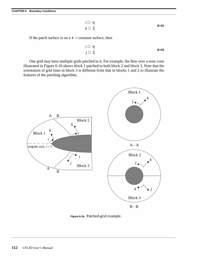
One grid may have multiple grids patched to it. For example, the flow over a nose coneillustrated in Figure6-16 shows block 1 patched to both block 2 and block 3. Note that theorientation of grid lines in block 3 is different from that in blocks 1 and 2 to illustrate thefeatures of the patching algorithm.

Figure 6-16. Patched-grid example.

i η⇔k ξ⇔

k

i η⇔j ξ⇔

k

i

k

i

j Block 3

Block 2

Block 1

A

AB

B

jk

jk

k j

Block 1

Block 2

Block 3

i

A - A

B - B

singular axis,i = 1



To provide two-way communication between all blocks, a total of seven interpolationsare required for this case, as follows:

The interpolations may be input in any order (but must be consistent once the order is cho-sen).

6.3.2.2Description/Discussion of Input Parameters

Basically, the patch algorithm works as follows. The interpolations are cycled through,one at a time, so that at any given time there is one surface being interpolated to. Note,however, that there may be more than one surface being interpolated from. In order tointerpolate from one (or more) block(s) to another, interpolation coefficients are required.These are found by expressing the cell-center coordinates on the “to” side of the

patch surface in terms of a nonlinear polynomial in , where are the local coordi-nates on the “from” side of the patch surface. Newton iteration is used to invert the poly-nomial to find the local coordinates of the cell center, .

Because of the nonlinearity of the equation, problems may arise in the iteration pro-cess. The parametersifit , limit , anditmax may be adjusted to try to overcome any conver-gence difficulties. There must beninter2 values for each of these three parameters.Limitis the maximum step size in or allowed during the search procedure. The value 1seems to be a good general choice.Itmax is the maximum number of search steps allowedper grid point. A rule of thumb is maximum dimension of, , oron a patch surface.

Ifit controls the order of the polynomial fit used to relate, , or to and . Ifit =

1 for linear in both and (bilinear).Ifit = 2 for quadratic in both and (degenerate

biquadratic).Ifit = 3 for quadratic in , linear in . Ifit = 4 for linear in , quadratic in .

Some tips for choosingifit are:

• A grid with highly curved grid lines in one of thelocal directions will need a quadraticpolynomial in that direction.

• Refer to Section6.3.2.1 and the user’s own knowledge of the grid to decide which (ifany) of the local directions or are highly curved.

• Use the lowest order fit which seems reasonable in each direction.

Interpolation: Description:1 To i = idim of block 1fromi = 1 of blocks 2 and 3 (two “from” blocks)2 To i = 1 of block 2fromi = idim of block 13 To i = 1 of block 3fromi = idim of block 14 To j = 1 of block 2fromk = 1 of block 35 To j = jdim of block 2fromk = kdim of block 36 To k = 1 of block 3fromj = 1 of block 27 To k = kdim of block 3fromj = jdim of block 2

xc yc zc, ,

ξ η, ξ η,

ξc ηc,

ξ η

limit itmax the≈× i j k

x y z ξ ηξ η ξ η

ξ η ξ η

ξ η



• One-to-one patching can always be done with a bilinear fit, regardless of curvature.

To andfrom are numbers containing attributes of the “to” side of the patch surface andthe “from” side of the patch surface. For each of theninter2 interpolations there is onlyone value ofto, but there may be more than one value offrom which is set by the parame-ter nfb. (Nfb is the number of blocks on the “from” side of the patch surface.) The valuesof to andfrom are of the form:

to/from = Nmn

where “N” indicates the block number; “m” indicates the coordinate which is constant onthe patch surface (may differ on either side of the patch):

and “n” indicates on which of the two possible m = constant surfaces the patch surfaceoccurs:

The following inputs pertain to the nose cone case in Figure6-16:

Interpolation # to nfb from1 112 2 211, 3112 211 1 1123 311 1 1124 221 1 331

m 1 i⇒ constant= =

m 2 j⇒ constant= =

m 3 k⇒ constant= =

n 1 for patch onm 1 surface= =

n 2 for patch onm mdim surface= =



Example

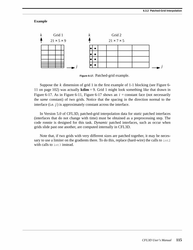
Suppose the dimension of grid 1 in the first example of 1-1 blocking (see Figure6-11 on page102) was actuallykdim = 9. Grid 1 might look something like that drawn inFigure6-17. As in Figure6-11, Figure6-17 shows an = constant face (not necessarilythe same constant) of two grids. Notice that the spacing in the direction normal to theinterface (i.e. ) is approximately constant across the interface.

In Version 5.0 of CFL3D, patched-grid interpolation data forstatic patched interfaces(interfaces that do not change with time) must be obtained as a preprocessing step. Thecode ronnie is designed for this task.Dynamic patched interfaces, such as occur whengrids slide past one another, are computed internally in CFL3D.

Note that, if two grids with very different sizes are patched together, it may be neces-sary to use a limiter on the gradients there. To do this, replace (hard-wire) the calls toint2

with calls toint3 instead.

Figure 6-17. Patched-grid example.

k k

j j

Grid 1 Grid 2

21 × 5 × 9 21 × 7 × 5

k

i

j



6.3.3Chimera Grid Interpolation

(Input Line Type Ten)

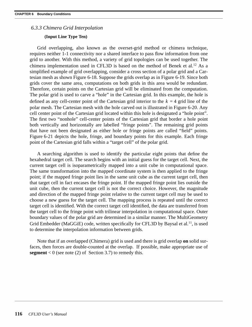
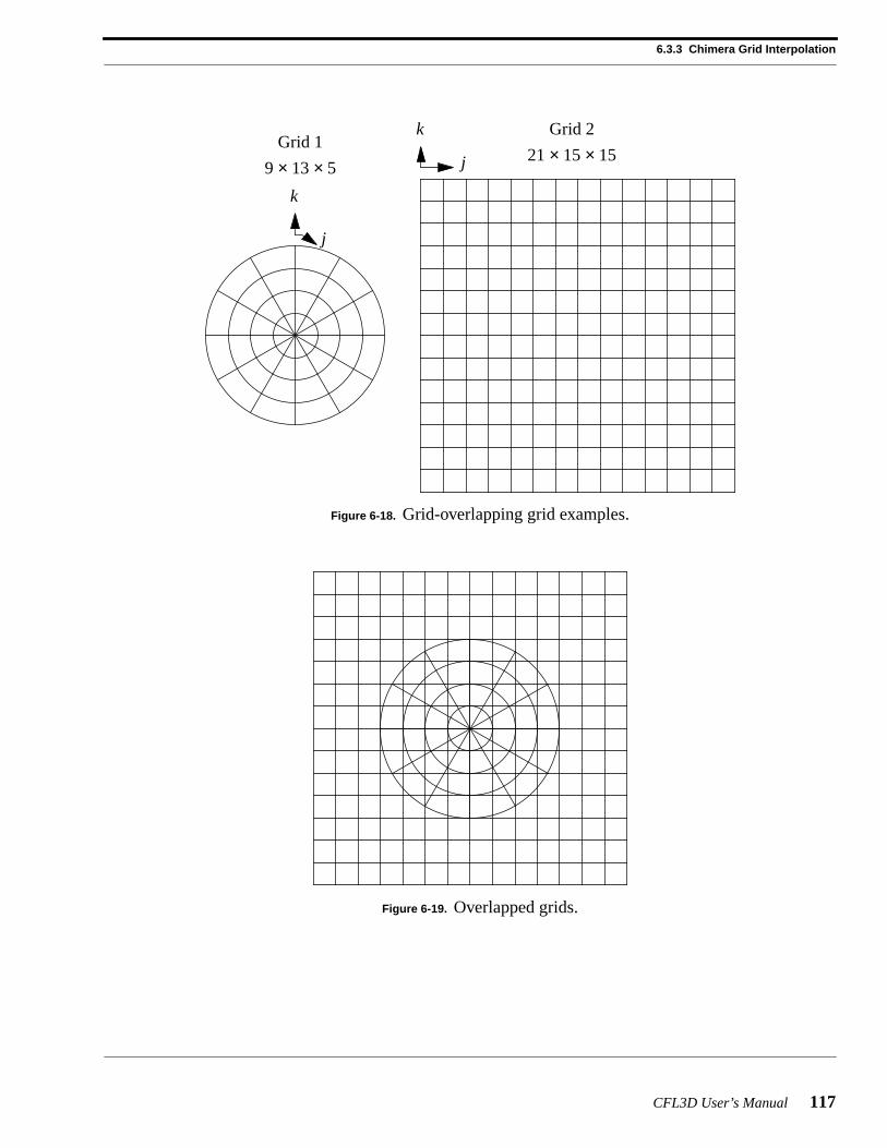
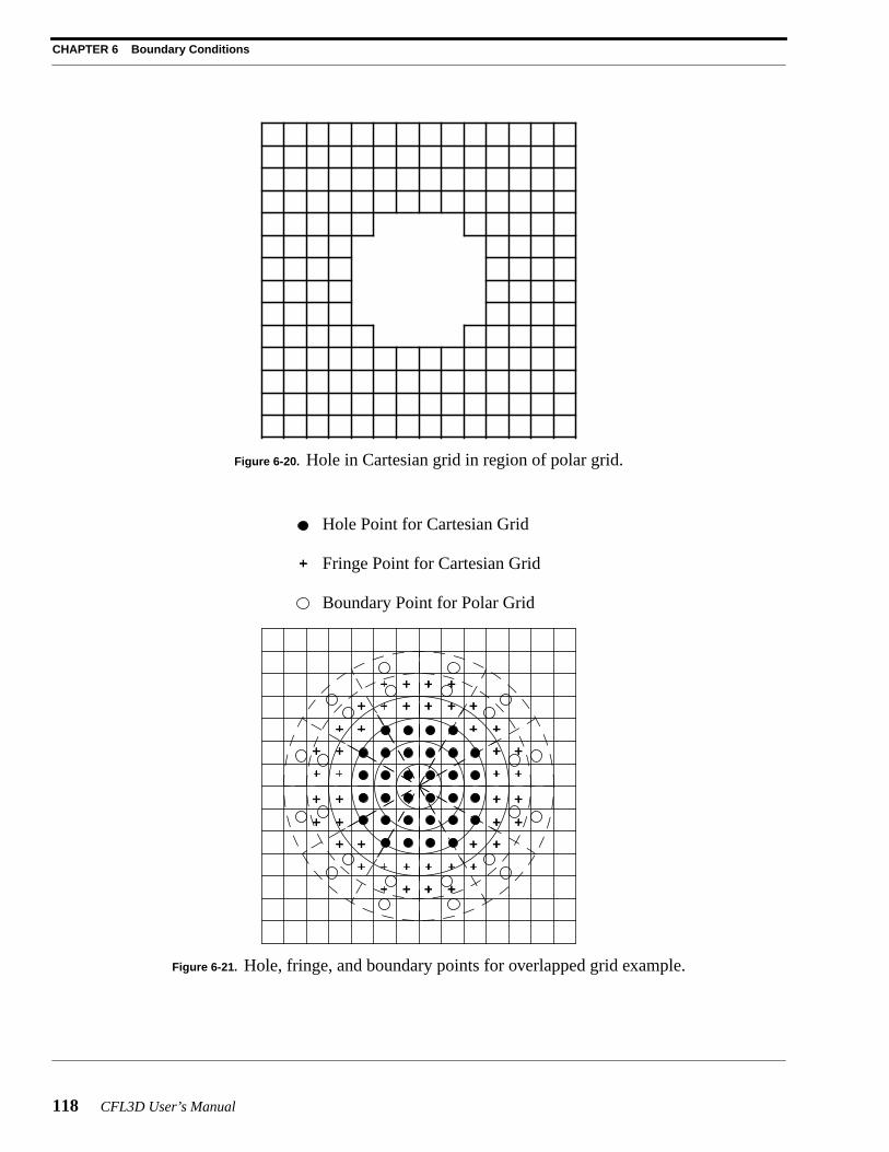
Grid overlapping, also known as the overset-grid method or chimera technique,requires neither 1-1 connectivity nor a shared interface to pass flow information from onegrid to another. With this method, a variety of grid topologies can be used together. Thechimera implementation used in CFL3D is based on the method of Benek et al.12 As asimplified example of grid overlapping, consider a cross section of a polar grid and a Car-tesian mesh as shown Figure6-18. Suppose the grids overlap as in Figure6-19. Since bothgrids cover the same area, computations on both grids in this area would be redundant.Therefore, certain points on the Cartesian grid will be eliminated from the computation.The polar grid is used to carve a “hole” in the Cartesian grid. In this example, the hole isdefined as any cell-center point of the Cartesian grid interior to the= 4 grid line of thepolar mesh. The Cartesian mesh with the hole carved out is illustrated in Figure6-20. Anycell center point of the Cartesian grid located within this hole is designated a “hole point”.The first two “nonhole” cell-center points of the Cartesian grid that border a hole pointboth vertically and horizontally are labelled “fringe points”. The remaining grid pointsthat have not been designated as either hole or fringe points are called “field” points.Figure6-21 depicts the hole, fringe, and boundary points for this example. Each fringepoint of the Cartesian grid falls within a “target cell” of the polar grid.

A searching algorithm is used to identify the particular eight points that define thehexahedral target cell. The search begins with an initial guess for the target cell. Next, thecurrent target cell is isoparametrically mapped into a unit cube in computational space.The same transformation into the mapped coordinate system is then applied to the fringepoint; if the mapped fringe point lies in the same unit cube as the current target cell, thenthat target cell in fact encases the fringe point. If the mapped fringe point lies outside theunit cube, then the current target cell is not the correct choice. However, the magnitudeand direction of the mapped fringe point relative to the current target cell may be used tochoose a new guess for the target cell. The mapping process is repeated until the correcttarget cell is identified. With the correct target cell identified, the data are transferred fromthe target cell to the fringe point with trilinear interpolation in computational space. Outerboundary values of the polar grid are determined in a similar manner. The MultiGeometryGrid Embedder (MaGGiE) code, written specifically for CFL3D by Baysal et al.11, is usedto determine the interpolation information between grids.

Note that if an overlapped (Chimera) grid is used and there is grid overlapon solid sur-faces, then forces are double-counted at the overlap. If possible, make appropriate use ofsegment < 0 (see note (2) of Section3.7) to remedy this.

k


6.3.3 Chimera Grid Interpolation

Figure 6-18. Grid-overlapping grid examples.

Figure 6-19. Overlapped grids.

j

k

k

j

Grid 1Grid 2

9 × 13 × 521 × 15 × 15



Figure 6-20. Hole in Cartesian grid in region of polar grid.

Figure 6-21. Hole, fringe, and boundary points for overlapped grid example.

Hole Point for Cartesian Grid

Fringe Point for Cartesian Grid

Boundary Point for Polar Grid


6.3.4 Embedded Mesh

6.3.4Embedded Mesh

Regular refinement of coarse mesh

Embedded grids are useful when high gradient areas are limited to an identifiableregion (see reference 25). An embedded grid can be placed in that region to resolve theflow field without refining the entire mesh. As an example, an embedded grid scheme isshown in Figure6-22 for two dimensions. The diagram represents full refinement in bothdirections. The solid lines define a finer mesh embedded completely within a coarser meshdepicted by the dashed lines. In the figure, a portion of the flow field is covered by both theembedded mesh and a portion of the coarser grid. The grids are coupled together duringthe solution process. The cell-center variables on a coarser grid cell which underlies a finerembedded grid cell are replaced with a volume-weighted restriction of variables from thefour (2-d) or eight (3-d) finer grid cells, similar to the restriction operators used in a globalmultigrid scheme.

For the embedded grid, the computational boundaries occur either at a physical bound-ary, such as a wing, a symmetry plane, an inflow/outflow plane along a zonal interface(one-to-one, patched, or overset), or along an interior computational surface of a coarsergrid. Along an interior surface, two additional lines of data corresponding to an analyticalcontinuation of the finer grid cell centers are constructed from linear interpolation of thecoarser grid state variables. An enlarged view of the lower-left corner of the embedded

Figure 6-22. Embedded grid example.

Embedded Grid Cell-Center Point

Embedded Grid Boundary Point

Global Grid Cell-Center Point



mesh of Figure6-22 is shown in Figure6-23. Arrows indicate which coarse grid points areused in the linear interpolation scheme to obtain a couple of the boundary points drawn. Ifthe input parametericonsf = 1 (“LT20 - Mesh Sequencing and Multigrid”), then globalconservation is enforced by replacing the coarse grid flux at an embedded grid boundarywith the sum of the finer grid fluxes which share the common interface. Ificonsf = 0, thecoarse grid flux is computed using the volume-weighted restriction from the fine grid, andconservation is not insured.

When designing an embedded mesh, it is important to remember that at least two lay-ers of coarse grid cells should surround the embedded boundaries unless the embeddedboundary is set with a physical boundary condition (e.g. solid wall, plane of symmetry, orfar-field) or a zonal boundary such as a one-to-one, patched, or overset type. In the exam-ple of Figure6-22, there are two layers of coarse grid cells above and below the embeddedmesh and three layers of coarse grid cells on the left and right sides of the embeddedmesh.

Suppose the grids in Figure6-22 are in an = constant plane. Also,jdim = 9 andkdim = 7 for the coarse grid andjdim = 5 andkdim = 5 for the embedded mesh. The per-tinent input would look something like:

Figure 6-23. Enlarged portion of embedded mesh.

Embedded Grid Cell-Center Point

Embedded Grid Boundary Point

Global Grid Cell-Center Point

i


6.3.4 Embedded Mesh


2 1 0 100 0 0 1 17 NCG IEM IADVANCE IFORCE IVISC(I) IVISC(J) IVISC(K)

0 0 0 0 0 0 00 1 0 0 0 0 0


10 INEWG IGRIDC IS JS KS IE JE KE0 0 0 0 0 0 0 00 1 1 4 3 21 6 5

20 MSEQ MGFLAG ICONSF MTT NGAM1 0 1 0 0

22 NCYC MGLEVG NEMBL NITFO1 1 1 0

In this example, the embedded mesh extends the entire length of the global grid in the direction. The dimensions of the embedded mesh must satisfy a particular relationship to

the data in “LT10 - Embedded Mesh Specifications”. The input parametersis, ie, js, je, ks,andke are indices in the global grid to which the embedded mesh is connected. Thus, thefollowing must be true:

(6-44)

Analogous relationships hold for the and directions. Note that the only exception to

Equation (6-44) occurs in the direction for 2-d cases, whereis = 2, ie = 1 and

.

There is also an option called “semi-coarsening” in which the number of points in the direction are the same for the embedded grid and the global grid in the embedded region.

This is helpful if there are sufficient points in the direction, but grid enrichment inplanes is desirable. There is an internal check for this option and the only change in theinput sample above is to setidim = 21 for the embedded grid as well. Note that semi-coarsening can only be used in the direction.

Another nice option with grid embedding is to add an embedded grid to a previously-run coarse grid problem. For instance, suppose a converged coarse grid solution isobtained and the flow field looks well resolved everywhere except in a vortex region. Anembedded grid for that region can be tacked on to the original grid file and the caserestarted. On thefirst run of the restart, setinewg = 1 for the embedded grid. This lets thecode know that a solution not on the current restart file is beginning. On the next run, theembedded grid solutionwill be on the restart file, so setinewg = 0.

i

idimembedded 2 ie is–( )global 1+=

j k

i

idimembedded idimglobal 2= =

i

i j k–

i



Date post:	10-Feb-2022
Category:	Documents
Upload:	others
View:	6 times
Download:	0 times

CHAPTER 6 Boundary Conditions - CFL3D

Documents