October 25, 2013 Data Mining: Concepts and Techniques 1 Chapter 6. Classification and Prediction What is classification? What is prediction? Issues regarding classification and prediction Classification by decision tree induction Classification by back propagation Lazy learners (or learning from your neighbors) Frequent-pattern-based classification Other classification methods Prediction Accuracy and error measures
Transcript
October 25, 2013 Data Mining: Concepts and Techniques 1
Chapter 6. Classification and Prediction
� What is classification? What is
prediction?
� Issues regarding classification and
prediction
� Classification by decision tree
induction
� Classification by back propagation
� Lazy learners (or learning from
your neighbors)
� Frequent-pattern-based
classification
� Other classification methods
� Prediction
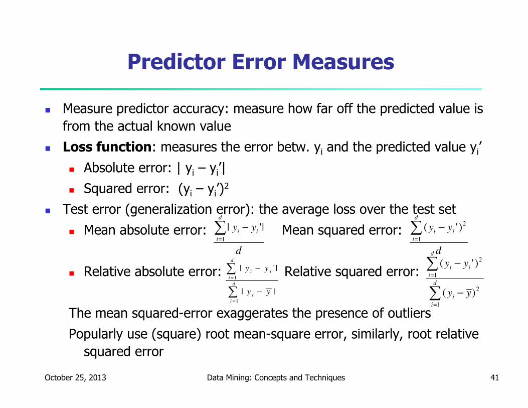
� Accuracy and error measures
October 25, 2013 Data Mining: Concepts and Techniques 2
Supervised vs. Unsupervised Learning
� Supervised learning (classification)
� Supervision: The training data (observations,
measurements, etc.) are accompanied by labels
indicating the class of the observations
� New data is classified based on the training set
� Unsupervised learning (clustering)
� The class labels of training data is unknown
� Given a set of measurements, observations, etc. with
the aim of establishing the existence of classes or
clusters in the data
October 25, 2013 Data Mining: Concepts and Techniques 3
� Classification
� predicts categorical class labels (discrete or nominal)
� classifies data (constructs a model) based on the training set and the values (class labels) in a classifying attribute and uses it in classifying new data
� Prediction
� models continuous-valued functions, i.e., predicts unknown or missing values
� Typical applications
� Credit/loan approval:
� Medical diagnosis: if a tumor is cancerous or benign
� Fraud detection: if a transaction is fraudulent
� Web page categorization: which category it is
Classification vs. Prediction
October 25, 2013 Data Mining: Concepts and Techniques 4
Classification—A Two-Step Process
� Model construction: describing a set of predetermined classes
� Each tuple/sample is assumed to belong to a predefined class, as determined by the class label attribute
� The set of tuples used for model construction is training set
� The model is represented as classification rules, decision trees, or mathematical formulae
� Model usage: for classifying future or unknown objects
� Estimate accuracy of the model
� The known label of test sample is compared with the classified result from the model
� Accuracy rate is the percentage of test set samples that are correctly classified by the model
� Test set is independent of training set, otherwise over-fitting will occur
� If the accuracy is acceptable, use the model to classify datatuples whose class labels are not known
October 25, 2013 Data Mining: Concepts and Techniques 5
Process (1): Model Construction
Training
Data
NAME RANK YEARS TENURED
Mike Assistant Prof 3 no
Mary Assistant Prof 7 yes
Bill Professor 2 yes
Jim Associate Prof 7 yes
Dave Assistant Prof 6 no
Anne Associate Prof 3 no
Classification
Algorithms
IF rank = ‘professor’
OR years > 6
THEN tenured = ‘yes’
Classifier
(Model)
October 25, 2013 Data Mining: Concepts and Techniques 6
Process (2): Using the Model in Prediction
Classifier
Testing
Data
NAME RANK YEARS TENURED
Tom Assistant Prof 2 no
Merlisa Associate Prof 7 no
George Professor 5 yes
Joseph Assistant Prof 7 yes
Unseen Data
(Jeff, Professor, 4)
Tenured?
October 25, 2013 Data Mining: Concepts and Techniques 7
Issues: Data Preparation
� Data cleaning
� Preprocess data in order to reduce noise and handle
missing values
� Relevance analysis (feature selection)
� Remove the irrelevant or redundant attributes
� Data transformation
� Generalize and/or normalize data
October 25, 2013 Data Mining: Concepts and Techniques 8
Issues: Evaluating Classification Methods
� Accuracy
� classifier accuracy: predicting class label
� predictor accuracy: guessing value of predicted attributes
� Speed
� time to construct the model (training time)
� time to use the model (classification/prediction time)
� Robustness: handling noise and missing values
� Scalability: efficiency in disk-resident databases
� Interpretability
� understanding and insight provided by the model
� Other measures, e.g., goodness of rules, such as decision tree size or compactness of classification rules
October 25, 2013 Data Mining: Concepts and Techniques 9
Decision Tree Induction: Training Dataset
age income student credit_rating buys_computer
<=30 high no fair no
<=30 high no excellent no
31…40 high no fair yes
>40 medium no fair yes
>40 low yes fair yes
>40 low yes excellent no
31…40 low yes excellent yes
<=30 medium no fair no
<=30 low yes fair yes
>40 medium yes fair yes
<=30 medium yes excellent yes
31…40 medium no excellent yes
31…40 high yes fair yes
>40 medium no excellent no
This follows an example of Quinlan’s ID3 (Playing Tennis)
October 25, 2013 Data Mining: Concepts and Techniques 10
Output: A Decision Tree for “buys_computer”
age?
overcast
student? credit rating?
<=30 >40
no yes yes
yes
31..40
no
fairexcellentyesno
October 25, 2013 Data Mining: Concepts and Techniques 11
Algorithm for Decision Tree Induction
� Basic algorithm (a greedy algorithm)
� Tree is constructed in a top-down recursive divide-and-conquer
manner
� At start, all the training examples are at the root
� Attributes are categorical (if continuous-valued, they are
discretized in advance)
� Examples are partitioned recursively based on selected attributes
� Test attributes are selected on the basis of a heuristic or
statistical measure (e.g., information gain)
� Conditions for stopping partitioning
� All samples for a given node belong to the same class
� There are no remaining attributes for further partitioning –
majority voting is employed for classifying the leaf
� There are no samples left
October 25, 2013 Data Mining: Concepts and Techniques 12
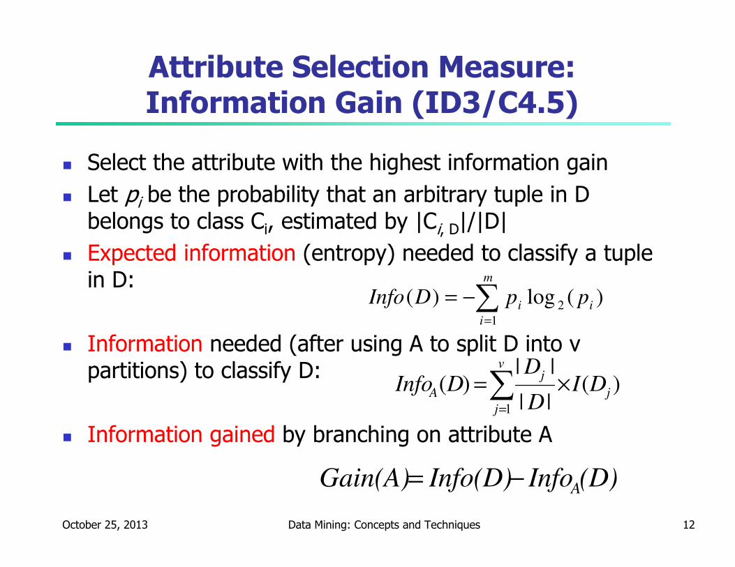
Attribute Selection Measure: Information Gain (ID3/C4.5)
� Select the attribute with the highest information gain
� Let pi be the probability that an arbitrary tuple in D belongs to class Ci, estimated by |Ci, D|/|D|
� Expected information (entropy) needed to classify a tuple in D:
� Information needed (after using A to split D into v partitions) to classify D:
� Information gained by branching on attribute A
)(log)( 2
1
i
m
i
i ppDInfo ∑=
−=
)(||
||)(
1
j
v
j
j
A DID
DDInfo ×=∑
=
(D)InfoInfo(D)Gain(A) A−=
October 25, 2013 Data Mining: Concepts and Techniques 13
Attribute Selection: Information Gain
g Class P: buys_computer = “yes”
g Class N: buys_computer = “no”
means “age <=30” has 5
out of 14 samples, with 2 yes’es
and 3 no’s. Hence
Similarly,
age pi ni I(pi, ni)
<=30 2 3 0.971
31…40 4 0 0
>40 3 2 0.971
694.0)2,3(14
5
)0,4(14
4)3,2(
14
5)(
=+
+=
I
IIDInfo age
048.0)_(
151.0)(
029.0)(
=
=
=
ratingcreditGain
studentGain
incomeGain
246.0)()()( =−= DInfoDInfoageGain ageage income student credit_rating buys_computer
<=30 high no fair no
<=30 high no excellent no
31…40 high no fair yes
>40 medium no fair yes
>40 low yes fair yes
>40 low yes excellent no
31…40 low yes excellent yes
<=30 medium no fair no
<=30 low yes fair yes
>40 medium yes fair yes
<=30 medium yes excellent yes
31…40 medium no excellent yes
31…40 high yes fair yes
>40 medium no excellent no
)3,2(14
5I
940.0)14
5(log
14
5)
14
9(log
14
9)5,9()( 22 =−−== IDInfo
October 25, 2013 Data Mining: Concepts and Techniques 14
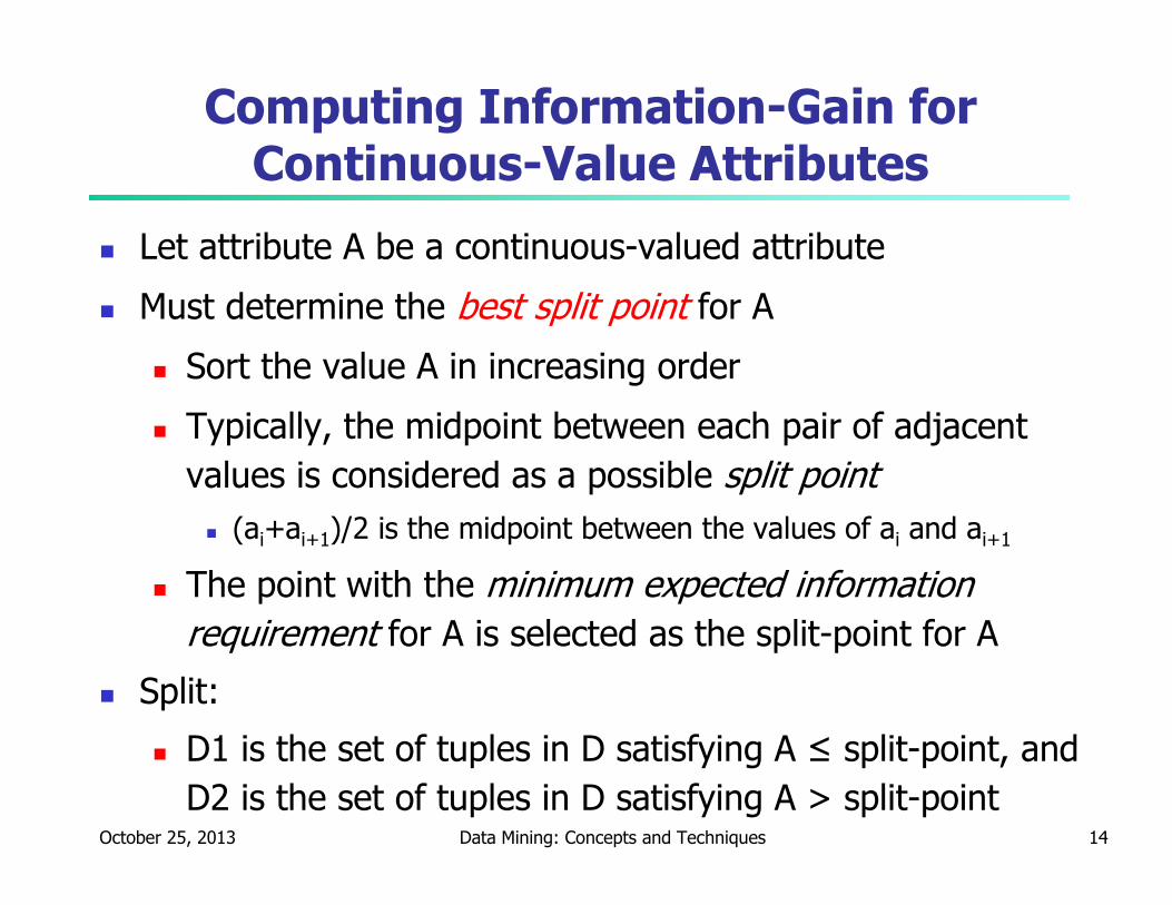
Computing Information-Gain for Continuous-Value Attributes
� Let attribute A be a continuous-valued attribute
� Must determine the best split point for A
� Sort the value A in increasing order
� Typically, the midpoint between each pair of adjacent
values is considered as a possible split point
� (ai+ai+1)/2 is the midpoint between the values of ai and ai+1
� The point with the minimum expected information
requirement for A is selected as the split-point for A
� Split:
� D1 is the set of tuples in D satisfying A ≤ split-point, and
D2 is the set of tuples in D satisfying A > split-point
October 25, 2013 Data Mining: Concepts and Techniques 15
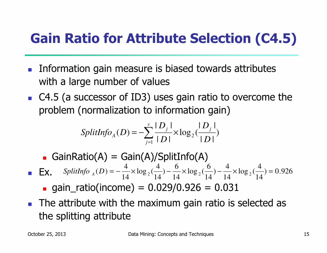
Gain Ratio for Attribute Selection (C4.5)
� Information gain measure is biased towards attributes
with a large number of values
� C4.5 (a successor of ID3) uses gain ratio to overcome the
problem (normalization to information gain)
� GainRatio(A) = Gain(A)/SplitInfo(A)
� Ex.
� gain_ratio(income) = 0.029/0.926 = 0.031
� The attribute with the maximum gain ratio is selected as
the splitting attribute
)||
||(log
||
||)( 2
1 D
D
D
DDSplitInfo
jv
j
j
A ×−= ∑=
926.0)14
4(log
14
4)
14
6(log
14
6)
14
4(log
14
4)( 222 =×−×−×−=DSplitInfo A
October 25, 2013 Data Mining: Concepts and Techniques 16
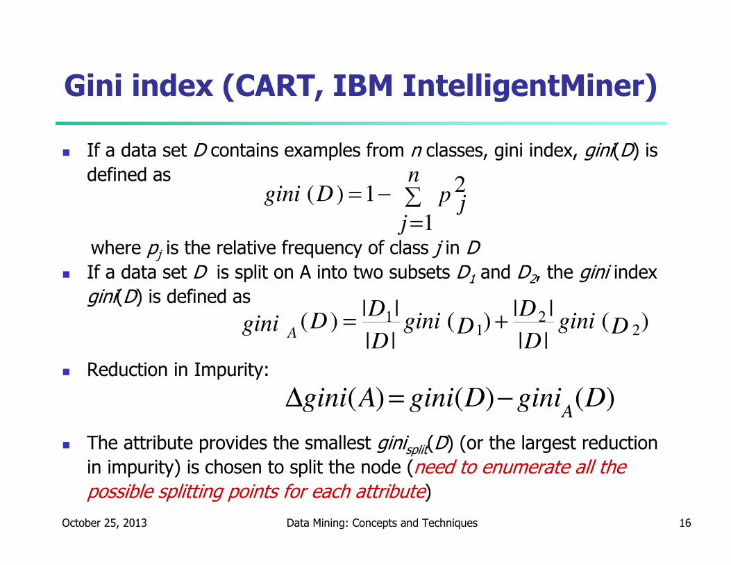
Gini index (CART, IBM IntelligentMiner)
� If a data set D contains examples from n classes, gini index, gini(D) is
defined as
where pj is the relative frequency of class j in D
� If a data set D is split on A into two subsets D1 and D2, the gini index
gini(D) is defined as
� Reduction in Impurity:
� The attribute provides the smallest ginisplit(D) (or the largest reduction
in impurity) is chosen to split the node (need to enumerate all the
possible splitting points for each attribute)
∑=
−=n
j
p jDgini
1
21)(
)(||
||)(
||
||)( 2
21
1Dgini
D
DDgini
D
DDgini A
+=
)()()( DginiDginiAginiA
−=∆
October 25, 2013 Data Mining: Concepts and Techniques 17
Gini index (CART, IBM IntelligentMiner)
� Ex. D has 9 tuples in buys_computer = “yes” and 5 in “no”
� Suppose the attribute income partitions D into 10 in D1: {low,
medium} and 4 in D2
but gini{medium,high} is 0.30 and thus the best since it is the lowest
� All attributes are assumed continuous-valued
� May need other tools, e.g., clustering, to get the possible split values
� Can be modified for categorical attributes
459.014
5
14
91)(
22
=
−
−=Dgini
)(14
4)(
14
10)( 11},{ DGiniDGiniDgini mediumlowincome
+
=∈
October 25, 2013 Data Mining: Concepts and Techniques 18
Comparing Attribute Selection Measures
� The three measures, in general, return good results but
� Information gain:
� biased towards multivalued attributes
� Gain ratio:
� tends to prefer unbalanced splits in which one
partition is much smaller than the others
� Gini index:
� biased to multivalued attributes
� has difficulty when # of classes is large
� tends to favor tests that result in equal-sized
partitions and purity in both partitions
October 25, 2013 Data Mining: Concepts and Techniques 19
Overfitting and Tree Pruning
� Overfitting: An induced tree may overfit the training data
� Too many branches, some may reflect anomalies due to noise or
outliers
� Poor accuracy for unseen samples
� Two approaches to avoid overfitting
� Prepruning: Halt tree construction early—do not split a node if this
would result in the goodness measure falling below a threshold
� Difficult to choose an appropriate threshold
� Postpruning: Remove branches from a “fully grown” tree—get a
sequence of progressively pruned trees
� Use a set of data different from the training data to decide
which is the “best pruned tree”
October 25, 2013 Data Mining: Concepts and Techniques 20
Classification in Large Databases
� Classification—a classical problem extensively studied by
statisticians and machine learning researchers
� Scalability: Classifying data sets with millions of examples
and hundreds of attributes with reasonable speed
� Why decision tree induction in data mining?
� relatively faster learning speed (than other classification methods)
� convertible to simple and easy to understand classification rules
� can use SQL queries for accessing databases
� comparable classification accuracy with other methods
October 25, 2013 Data Mining: Concepts and Techniques 21
Classification by Backpropagation
� Backpropagation: A neural network learning algorithm
� Started by psychologists and neurobiologists to develop
and test computational analogues of neurons
� A neural network: A set of connected input/output units
where each connection has a weight associated with it
� During the learning phase, the network learns by
adjusting the weights so as to be able to predict the
correct class label of the input tuples
� Also referred to as connectionist learning due to the
connections between units
October 25, 2013 Data Mining: Concepts and Techniques 22
Neural Network as a Classifier
� Weakness
� Long training time
� Require a number of parameters typically best determined empirically, e.g., the network topology or “structure.”
� Poor interpretability: Difficult to interpret the symbolic meaning behind the learned weights and of “hidden units” in the network
� Strength
� High tolerance to noisy data
� Ability to classify untrained patterns
� Well-suited for continuous-valued inputs and outputs
� Successful on a wide array of real-world data
� Algorithms are inherently parallel
� Techniques have recently been developed for the extraction of rules from trained neural networks
October 25, 2013 Data Mining: Concepts and Techniques 23
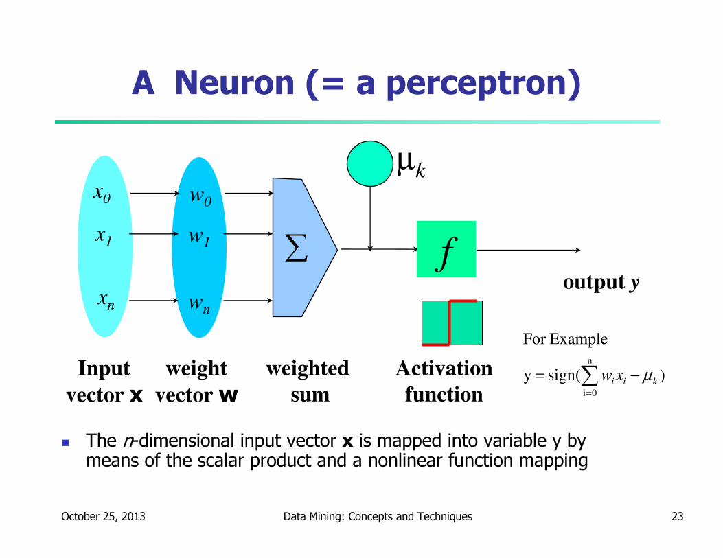
A Neuron (= a perceptron)
� The n-dimensional input vector x is mapped into variable y by means of the scalar product and a nonlinear function mapping
µk-
f
weighted
sum
Input
vector x
output y
Activation
function
weight
vector w
∑
w0
w1
wn
x0
x1
xn
)sign(y
ExampleFor
n
0i
kii xw µ−= ∑=
October 25, 2013 Data Mining: Concepts and Techniques 24
A Multi-Layer Feed-Forward Neural Network
Output layer
Input layer
Hidden layer
Output vector
Input vector: X
wij
ij
k
ii
k
j
k
j xyyww )ˆ( )()()1( −+=+ λ
October 25, 2013 Data Mining: Concepts and Techniques 25
How A Multi-Layer Neural Network Works?
� The inputs to the network correspond to the attributes measured
for each training tuple
� Inputs are fed simultaneously into the units making up the input
layer
� They are then weighted and fed simultaneously to a hidden layer
� The number of hidden layers is arbitrary, although usually only one
� The weighted outputs of the last hidden layer are input to units
making up the output layer, which emits the network's prediction
� The network is feed-forward in that none of the weights cycles
back to an input unit or to an output unit of a previous layer
� From a statistical point of view, networks perform nonlinear
regression: Given enough hidden units and enough training
samples, they can closely approximate any function
October 25, 2013 Data Mining: Concepts and Techniques 26
Defining a Network Topology
� First decide the network topology: # of units in the
input layer, # of hidden layers (if > 1), # of units in each
hidden layer, and # of units in the output layer
� Normalizing the input values for each attribute measured in
the training tuples to [0.0—1.0]
� One input unit per domain value, each initialized to 0
� Output, if for classification and more than two classes,
one output unit per class is used
� Once a network has been trained and its accuracy is
unacceptable, repeat the training process with a different
network topology or a different set of initial weights
October 25, 2013 Data Mining: Concepts and Techniques 27
Backpropagation
� Iteratively process a set of training tuples & compare the network's
prediction with the actual known target value
� For each training tuple, the weights are modified to minimize the
mean squared error between the network's prediction and the
actual target value
� Modifications are made in the “backwards” direction: from the output
layer, through each hidden layer down to the first hidden layer, hence
“backpropagation”
� Steps
� Initialize weights (to small random #s) and biases in the network
� Propagate the inputs forward (by applying activation function)
� Backpropagate the error (by updating weights and biases)
� Terminating condition (when error is very small, etc.)
October 25, 2013 Data Mining: Concepts and Techniques 28
Backpropagation and Interpretability
� Efficiency of backpropagation: Each epoch (one interation through the
training set) takes O(|D| * w), with |D| tuples and w weights, but # of
epochs can be exponential to n, the number of inputs, in the worst
case
� Rule extraction from networks: network pruning
� Simplify the network structure by removing weighted links that
have the least effect on the trained network
� Then perform link, unit, or activation value clustering
� The set of input and activation values are studied to derive rules
describing the relationship between the input and hidden unit
layers
� Sensitivity analysis: assess the impact that a given input variable has
on a network output. The knowledge gained from this analysis can be
represented in rules
October 25, 2013 Data Mining: Concepts and Techniques 29
Lazy vs. Eager Learning
� Lazy vs. eager learning
� Lazy learning (e.g., instance-based learning): Simply stores training data (or only minor processing) and waits until it is given a test tuple
� Eager learning (the above discussed methods): Given a set of training set, constructs a classification model before receiving new (e.g., test) data to classify
� Lazy: less time in training but more time in predicting
� Accuracy
� Lazy method effectively uses a richer hypothesis space since it uses many local linear functions to form its implicit global approximation to the target function
� Eager: must commit to a single hypothesis that covers the entire instance space
October 25, 2013 Data Mining: Concepts and Techniques 30
Lazy Learner: Instance-Based Methods
� Instance-based learning:
� Store training examples and delay the processing (“lazy evaluation”) until a new instance must be classified
� Typical approaches
� k-nearest neighbor approach
� Instances represented as points in a Euclidean space.
� Locally weighted regression
� Constructs local approximation
� Case-based reasoning
� Uses symbolic representations and knowledge-based inference
October 25, 2013 Data Mining: Concepts and Techniques 31
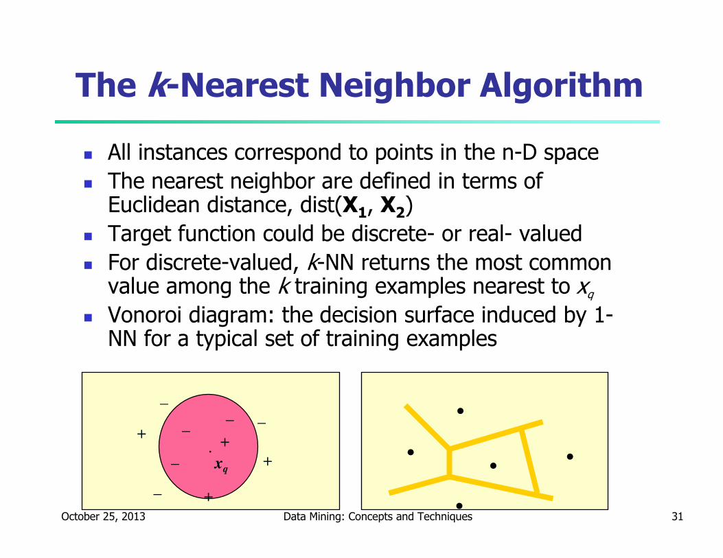
The k-Nearest Neighbor Algorithm
� All instances correspond to points in the n-D space
� The nearest neighbor are defined in terms of Euclidean distance, dist(X1, X2)
� Target function could be discrete- or real- valued
� For discrete-valued, k-NN returns the most common value among the k training examples nearest to xq
� Vonoroi diagram: the decision surface induced by 1-NN for a typical set of training examples
.
_+
_ xq
+
_ _+
_
_
+
.
..
. .
October 25, 2013 Data Mining: Concepts and Techniques 32
Discussion on the k-NN Algorithm
� k-NN for real-valued prediction for a given unknown tuple
� Returns the mean values of the k nearest neighbors
� Distance-weighted nearest neighbor algorithm
� Weight the contribution of each of the k neighbors
according to their distance to the query xq
� Give greater weight to closer neighbors
� Robust to noisy data by averaging k-nearest neighbors
� Curse of dimensionality: distance between neighbors could
be dominated by irrelevant attributes
� To overcome it, axes stretch or elimination of the least
relevant attributes
2),(
1
ixqxd
w≡
October 25, 2013 Data Mining: Concepts and Techniques 33
Genetic Algorithms (GA)
� Genetic Algorithm: based on an analogy to biological evolution
� An initial population is created consisting of randomly generated rules
� Each rule is represented by a string of bits
� E.g., if A1 and ¬A2 then C2 can be encoded as 100
� If an attribute has k > 2 values, k bits can be used
� Based on the notion of survival of the fittest, a new population is
formed to consist of the fittest rules and their offsprings
� The fitness of a rule is represented by its classification accuracy on a
set of training examples
� Offsprings are generated by crossover and mutation
� The process continues until a population P evolves when each rule in P
satisfies a prespecified threshold
� Slow but easily parallelizable
October 25, 2013 Data Mining: Concepts and Techniques 34
What Is Prediction?
� (Numerical) prediction is similar to classification
� construct a model
� use model to predict continuous or ordered value for a given input
� Prediction is different from classification
� Classification refers to predict categorical class label
� Prediction models continuous-valued functions
� Major method for prediction: regression
� model the relationship between one or more independent or predictor variables and a dependent or response variable
� Regression analysis
� Linear and multiple regression
� Non-linear regression
� Other regression methods: generalized linear model, Poisson regression, log-linear models, regression trees
October 25, 2013 Data Mining: Concepts and Techniques 35
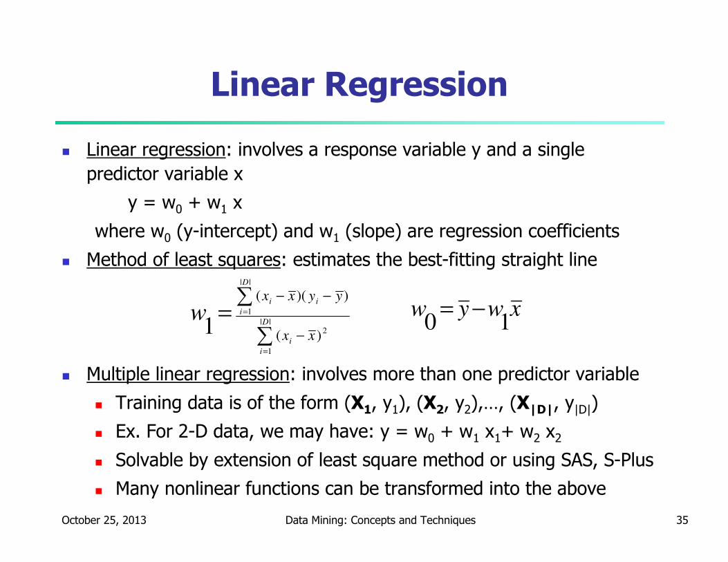
Linear Regression
� Linear regression: involves a response variable y and a single
predictor variable x
y = w0 + w1 x
where w0 (y-intercept) and w1 (slope) are regression coefficients
� Method of least squares: estimates the best-fitting straight line
� Multiple linear regression: involves more than one predictor variable
� Training data is of the form (X1, y1), (X2, y2),…, (X|D|, y|D|)
� Ex. For 2-D data, we may have: y = w0 + w1 x1+ w2 x2
� Solvable by extension of least square method or using SAS, S-Plus
� Many nonlinear functions can be transformed into the above
∑
∑
=
=
−
−−
=||
1
2
||
1
)(
))((
1 D
i
i
D
i
ii
xx
yyxx
w xwyw10
−=
October 25, 2013 Data Mining: Concepts and Techniques 36
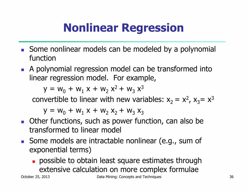
� Some nonlinear models can be modeled by a polynomial function
� A polynomial regression model can be transformed into linear regression model. For example,
y = w0 + w1 x + w2 x2 + w3 x3
convertible to linear with new variables: x2 = x2, x3= x3
y = w0 + w1 x + w2 x2 + w3 x3
� Other functions, such as power function, can also be transformed to linear model
� Some models are intractable nonlinear (e.g., sum of exponential terms)
� possible to obtain least square estimates through extensive calculation on more complex formulae
Nonlinear Regression
October 25, 2013 Data Mining: Concepts and Techniques 37
� Generalized linear model:
� Foundation on which linear regression can be applied to modeling
categorical response variables
� Variance of y is a function of the mean value of y, not a constant
� Logistic regression: models the prob. of some event occurring as a
linear function of a set of predictor variables
� Poisson regression: models the data that exhibit a Poisson