292

CHAPTER 6: ESTIMATION

6.1 LINEAR ESTIMATION

6.1.1 Introduction

Most estimation problems involve an output vector Y that is to be determined from: 1) an observed input vector X of any length, and 2) apriori information about the relationship of X to Y. Often the apriori information is training data consisting of a finite representative ensemble of vector pairs {X,Y}. In some cases the vectors x and y form a time series with additional constraints relating successive vectors. This chapter addresses two types of estimation problems: those where the statistical relationship is known and those where it must be deduced from limited observations. The related topic of hypothesis testing was treated in the context of communications in Chapter 4. Section 6.1 emphasizes linear estimation methods, while Section 6.2 treats representative nonlinear techniques.

The three illustrative linear estimation problems treated in Section 6.1 involve: 1) a linear problem with a known relationship between input and output; this example involves reduction of the systematic blurring introduced in most imaging systems, 2) a similar problem but with known non-linear physics and non-jointly-Gaussian statistics; where the object is to remotely sense the 3-D state of a system like the terrestrial atmosphere from 2-D observations of microwave or optical spectra, and 3) a multiple regression problem where the physics and statistics are unknown and must be deduced from a given finite set of training observations, where this case is also often encountered in remote sensing problems. Section 6.2 then reviews non-linear estimation techniques for similar problems.

6.1.2 Linear Image Sharpening

One classic problem typical of many “deblurring” or “image sharpening” applications is that of estimating the true sky brightness distribution B ST as a function of the two-dimensional

source angle S (the overbar signifies a vector quantity). The finite resolution antenna is pointed

at angle A at any instant, and the antenna response to radiation arriving from the source angle

S depends on the antenna gain in that direction, A SG . If the radiation arriving from

different angles is uncorrelated, then the linear relationship (3.1.13) between sky brightness and antenna temperature A AT becomes:

4

SSBSAAA dTG41

T (6.1.1)

293

BTG41

(6.1.2)

where “*” signifies two-dimensional convolution. This characterization of blurring is also relevant to video, audio, and other applications.

If we Fourier transform (6.1.2) from angular coordinates into angular frequency

coordinates radian/cycless over a small solid angle of interest, we obtain an equation which

can readily be solved for BT s :

sTsG41

sT BA (6.1.3)

where the Fourier relationship for antenna gain is:

yxssj2

yxyx dde,Gs,sG yyxx (6.1.4)

A simple example illustrates how the desired but unknown brightness distribution BT

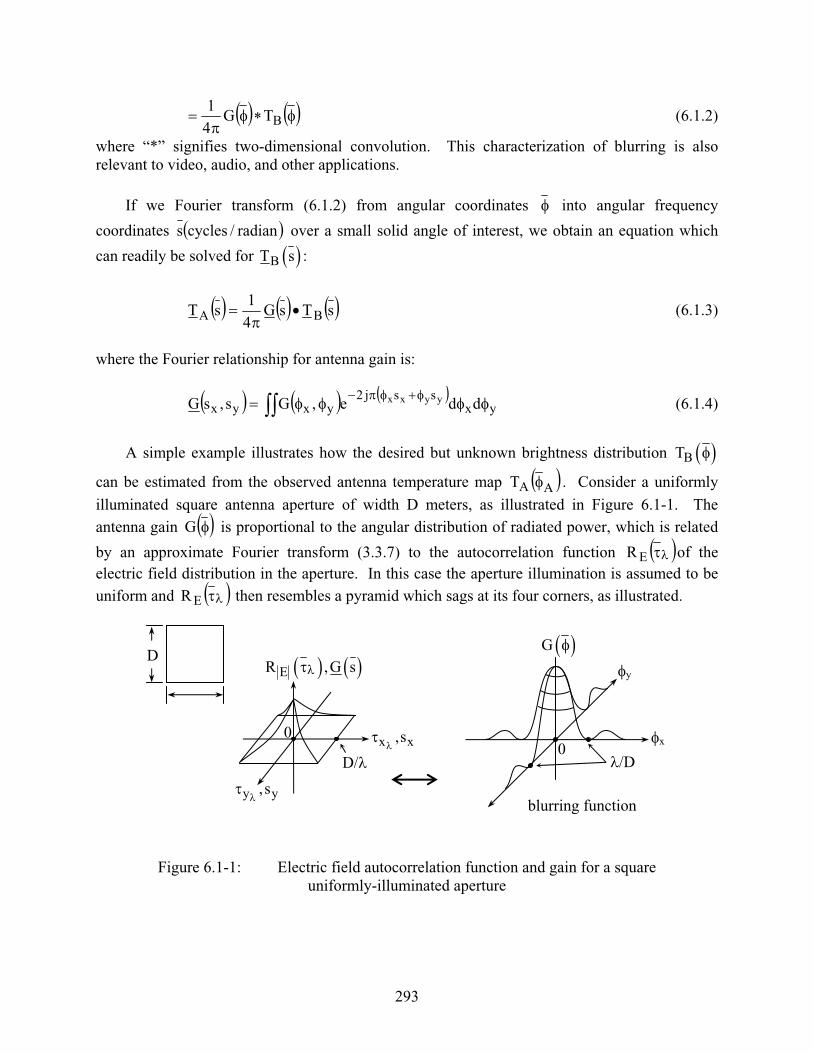
can be estimated from the observed antenna temperature map AAT . Consider a uniformly

illuminated square antenna aperture of width D meters, as illustrated in Figure 6.1-1. The antenna gain G is proportional to the angular distribution of radiated power, which is related

by an approximate Fourier transform (3.3.7) to the autocorrelation function ER of the electric field distribution in the aperture. In this case the aperture illumination is assumed to be uniform and ER then resembles a pyramid which sags at its four corners, as illustrated.

Figure 6.1-1: Electric field autocorrelation function and gain for a square uniformly-illuminated aperture

DER ,G s

D/x x,s0

y y,s

0x

y

G

blurring function

/D

294

Since the gain spectral characteristics sG and field autocorrelation function ER are both

Fourier transforms of the antenna gain G , they both have the same pyramidal shape, which

becomes zero beyond spatial offsets of D/ or angular frequencies s greater than D/ .Therefore we use the solution:

AB

4 T sT̂ s W s

G s (6.1.5)

where the window function sW avoids the singularity introduced at angular frequencies s for

which the gain is zero; the carot over a symbol indicates an estimate. That is, sW is zero when

sG is zero, and unity otherwise; in this case (6.1.5) is called the principal solution for the antenna deconvolution or “blurring” problem.

The nature of the principal solution is well illustrated by the example of a point source for which AT . In this case sTA = unity, and therefore our estimated brightness

temperature angular spectrum sWsT̂B , so that our estimated brightness temperature

distribution BT̂ is simply a two-dimensional sinc function, as illustrated in Figure 6.1-2.

Note that the first zero for the retrieved brightness distribution occurs at angle /2D, and that the solution BT̂ becomes negative at some angles. Obviously we can reduce the solution error by

setting every negative estimate of BT̂ to zero (a non-linear operation).

Figure 6.1-2 : Brightness temperature principal solution for a point source

A more serious problem with the principal solution arises because the observations are typically corrupted by additive noise:

BT̂

y

x

zero at /2D

Bpredicts T 0!

295

A AT̂ s T s N s (6.1.6)

For angular frequencies s where the signal-to-noise ratio is good, the noise perturbs the solution

only slightly. However, for angular frequencies s approaching D/ where both sG and sTA

approach zero, the noise sN typically has been amplified by sG4 to unacceptably high levels, destroying the utility of the solution, as suggested in Figure 6.1-3.

Figure 6.1-3: Point-source principal solution illustrating noise amplification

One remedy for excessively amplified noise is to optimize the weighting function W s , for example, by minimizing:

o

2

B AW s

ˆE T s T s N s QG s

(6.1.7)

By setting the derivative Q/ W = 0 and solving for the optimum weighting function, we obtain:

o o o

o

2A A A

optimum 2A

1 1E T T s N s T s N s2 2W sE T s N s

(6.1.8)

If we make the reasonable assumption that the antenna temperature and receiver noise

contributions are uncorrelated, i.e. AE T N 0 , then:

o

optimum 2 2A

1 1W s1 N S1 E N s E T s

(6.1.9)

Amplified white noise N s for small G s

DD

0

BT̂ s for point source

sx

296

where S and N are defined as the signal and noise power, respectively, and the weighting SN11 has broad utility.

In this case the boxcar form of the principal solution weighting function W s is modified; it tapers instead gently to zero near D/ where the signal-to-noise ratio deteriorates. For example, (6.1.9) suggests that at angular frequencies where the expected values of the noise and target powers are equal, the optimum weighting function equals 0.5. By apodizing the weighting function in this way the restored image is blurred but has lower sidelobes, an effect which may be desired even without considering the effects of noise.

The solution represented by (6.1.5) and (6.1.9) can be used for restoration of convolutionally blurred images of all types. For example, photographs, video images, radar images, filtered speech or music, and many other signal types can be restored in this simple fashion, provided the signal-to-noise ratio is acceptable at the frequencies of interest. A more difficult estimation problem results when the blurring function G of (6.1.1) is different for every A or portion of the observed signal, and where the blurring function may depend to some degree on the image itself. This is the case treated in Section 6.1.3.

6.1.3 Remote Sensing and Variable Blurring

An important problem which illustrates variable or data-dependent blurring functions is 3-D remote sensing, where an antenna or optimal sensor observes the brightness temperature (power spectrum) emitted by a deep medium where the parameter of interest, temperature for example, impacts the observation to a degree which depends on both depth in the medium and the wavelength which is observed. This dependence on depth is suggested by the equation of radiative transfer in the long wavelength limit (Rayleigh-Jeans approximation):

L

0

)z(BB dze)z()z(TeTKT o

o (6.1.10)

which corresponds to the simple geometry illustrated in Figure 6.1-4, and follows from (2.1.34). The optical depth (z) is defined as the integral of the absorption coefficient (z)(neper/meter) between observer and the depth z of interest:

L

z

dz)z()z( (6.1.11)

where we have defined o as the maximum optical depth corresponding to z = 0.

297

Figure 6.1-4: Slab geometry for characterizing the equation of radiative transfer

In general, the contribution from the surface attenuated by the overlying atmosphere, o

BoT e , includes contributions from the down-welling radiation reflected from the surface,

which typically has reflectivity R. In this case four contributions to the observed brightness temperature can be identified, as suggested in Figure 6.1-5.

Figure 6.1-5: Geometry of observed radiation, including reflected components

The first term (1) suggested in Figure 6.1-5 corresponds to the sky brightness sT , which is

reduced by the surface reflectivity R (R 1) and attenuated twice by the atmosphere o2e .Term (2) corresponds to radiation which is emitted downward by the atmosphere and then reflected from the surface. Term (3) is proportional to the ground temperature GT times the

surface emissivity ( < 1) attenuated once by the atmosphere oe , while term (4) corresponds to the direct emission by the atmosphere. That is:

T(z)

0

L

zBT K

oBT

1

2

TB

TS

TG

oe

R = 1 -

0

L

3

4

R

z

298

o

z

0oo eTdze)z()z(TReeRT)K(T G

L

0

dz)z(2

sB

dze)z()z(T

L

zdz)z(L

0

(6.1.12)

where the four terms in (6.1.12) are, in sequence, the four terms suggested graphically in Figure 6.1-5. In the limit where the atmosphere becomes opaque and unityo , (6.1.12) reduces to

the fourth term alone, which is equivalent to the second term on the right-hand side of (6.1.10). For specular surfaces, which are smooth and do not scatter, the surface reflectivity R = 1 - ,where is the corresponding specular emissivity in the same direction as the incident ray.

To use linear estimation techniques it is useful to put the equation of radiative transfer (6.1.12) into a simpler linear form. For the high-atmospheric-opacity case, (6.1.12) can be approximated as:

L

0oB dz)z(T,f,zW)z(TT)f(T (6.1.13)

where the first three terms of (6.1.12) have been combined into an equivalent brightness temperature oT . In general, those terms that combined to form the temperature weighting

function W(z,f,T(z)) in (6.1.13) have a weak dependence on that temperature profile T(z) that we are trying to estimate; W(z,f) is thus a data-dependent blurring function. To reduce the effects of this dependence it is sometimes useful to linearize about a presumed operating point To(z) for which there is a local incremental weighting function:

)z(T

Bo

o)z(T

T)z(T,f,zW (6.1.14)

In this case (6.1.13) becomes:

dz)z(T,f,zW)z(T)z(TT)f(T o

L

0ooB (6.1.15)

Equations (6.1.13) and (6.1.15) both define linear relationships between the observed brightness temperature spectrum )f(TB and the unknown T(z) that we hope to retrieve (the retrievalproblem.) This problem involves retrieving the unknown function TB(f) from a set of scalars,

299

each being the integral of the unknown over a weighting function unique to each observation. This problem statement is quite general and applicable to a wide variety of estimation problems.

It is clear that if the observations consist of a finite number of spectral samples, solutions to (6.1.13) or (6.1.15) are not unique if the number of degrees of freedom in T(z) exceeds the number N of independent spectral samples. This is often the case when retrieving temperature profiles, and for many other estimation problems. In any event, N generally differs from the number of degrees of freedom in the ensemble of possible temperature profiles T(z), and in their corresponding brightness temperature spectrum )f(TB .

First consider the nature of blurring in depth z for the case where the temperature profile T(z) is revealed by its resulting brightness spectrum. This variable blurring is characterized by the weighting functions W(z,f) of (6.1.13) and (6.1.15). These weighting functions are determined by the atmospheric absorption coefficient (f,P,T). We shall neglect the weak dependence of on temperature T in this discussion, and consider the dependence on pressure P to be dominated by pressure broadening, as explained below.

The dominant atmospheric absorption lines at microwave frequencies are the isolated water vapor resonances near 22.235 and 183.75 GHz, the isolated oxygen (O2) absorption line near 118.3 GHz, and the cluster of oxygen lines 50-70 GHz. Each of these lines can be modeled classically as being associated with a rotating molecule with a permanent electric or magnetic dipole moment, as discussed in Section 3.4. The frequency spectrum of these classical rotating dipole moments is a series of impulses each associated with a different quantum state of the molecule. These rotations and sinusoids are randomly interrupted and phase shifted by every molecular collision, yielding pressure broadened spectral lines with linewidths of approximately proportional to the number of significant collisions per second. These line shapes can be computed by taking the Fourier transform of a sinusoid with poisson-distributed phase-shift events randomly distributed over 2 .

The collision frequency and linewidth for a trace gas are proportional to pressure P if the

trace gas has a small constant mixing ratio, where mixing ratio is defined as the fraction of the

molecules associated with the spectral line of interest. This proportionality constant depends on

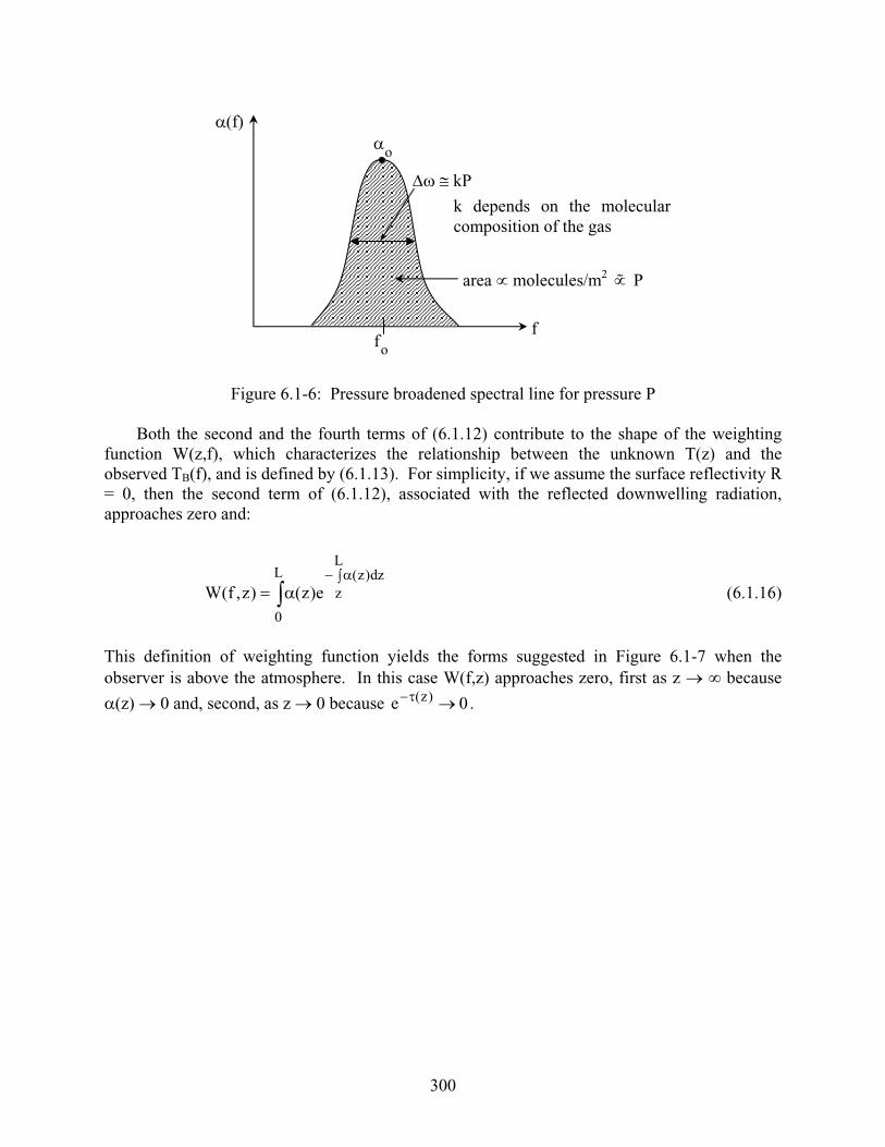
which two molecular species are colliding. As suggested in Figure 6.1-6, the area under an

absorption line is proportional to the number of absorbing molecules per meter.

300

Figure 6.1-6: Pressure broadened spectral line for pressure P

Both the second and the fourth terms of (6.1.12) contribute to the shape of the weighting function W(z,f), which characterizes the relationship between the unknown T(z) and the observed TB(f), and is defined by (6.1.13). For simplicity, if we assume the surface reflectivity R = 0, then the second term of (6.1.12), associated with the reflected downwelling radiation, approaches zero and:

L

zdz)z(L

0

e)z()z,f(W (6.1.16)

This definition of weighting function yields the forms suggested in Figure 6.1-7 when the observer is above the atmosphere. In this case W(f,z) approaches zero, first as z because

(z) 0 and, second, as z 0 because 0e )z( .

of

area molecules/m2 P

o

kP

k depends on the molecular composition of the gas

f

(f)

301

Figure 6.1-7: Absorption coefficients (z) and weighting functions W(z,f) for atmospheric temperature profiles observed from space

Because both the spectral linewidth f and the spectral line area are proportional to pressure P, the peak absorption coefficient (z) = o is independent of altitude up to those altitudes where the linewidth becomes roughly constant because it is so narrow that it is dominated instead by Doppler broadening and spontaneous emission. Above that altitude the peak absorption coefficient of and spectral line area decrease with pressure, as suggested in Figure 6.1-7 for

off , and W(f,z) approaches zero. At any frequency f the absorption coefficient (m-1)

approaches its peak o for pressures sufficiently great that the linewidth f substantially

exceeds the frequency difference off . At still lower altitudes the exponential factor in

(6.1.16) begins to dominate so that W(z,f) reaches a peak and then diminishes rapidly, as illustrated in Figure 6.1-7. The shape and width of the weighting function with altitude are therefore similar for all frequencies, and W is simply translated towards lower altitudes for frequencies increasingly removed from the center of the resonance. The peak of the weighting

function occurs for optical depth near unity, where L

1zf f ,z ' dz ' . The width of W in

altitude typically ranges between one and two pressure scale heights, depending in part on the mixing ratio and temperature dependence of the absorption coefficient; the pressure scale height for the troposphere is approximately 8 km.

The same expression (6.1.16) yields a different altitude dependence for weighting functions W(z,f) obtained when the observer is on the terrestrial surface looking upwards, as suggested in Figure 6.1-8. In this case (z) is unchanged, but both factors of (6.1.16), namely (z) and the exponential, decrease with altitude as does W(f,z). This decay rate is fastest for the resonant frequency of where the absorption coefficient is greatest. These weighting functions roughly

resemble decaying exponentials which, in the limit of low absorption coefficients, decay very slowly with altitude. For this up-looking geometry we can deduce temperature profiles with much greater accuracy very close to the observer, and with decreasing accuracy further away.

z

0

W(z,fo)f fo (maximum opacity)

f2 = fo 2

o(z)

W(z,f)

altitudes where intrinsic & doppler broadening dominate

f P

f1 fo 1W(z,f1)

W(z,f2)

302

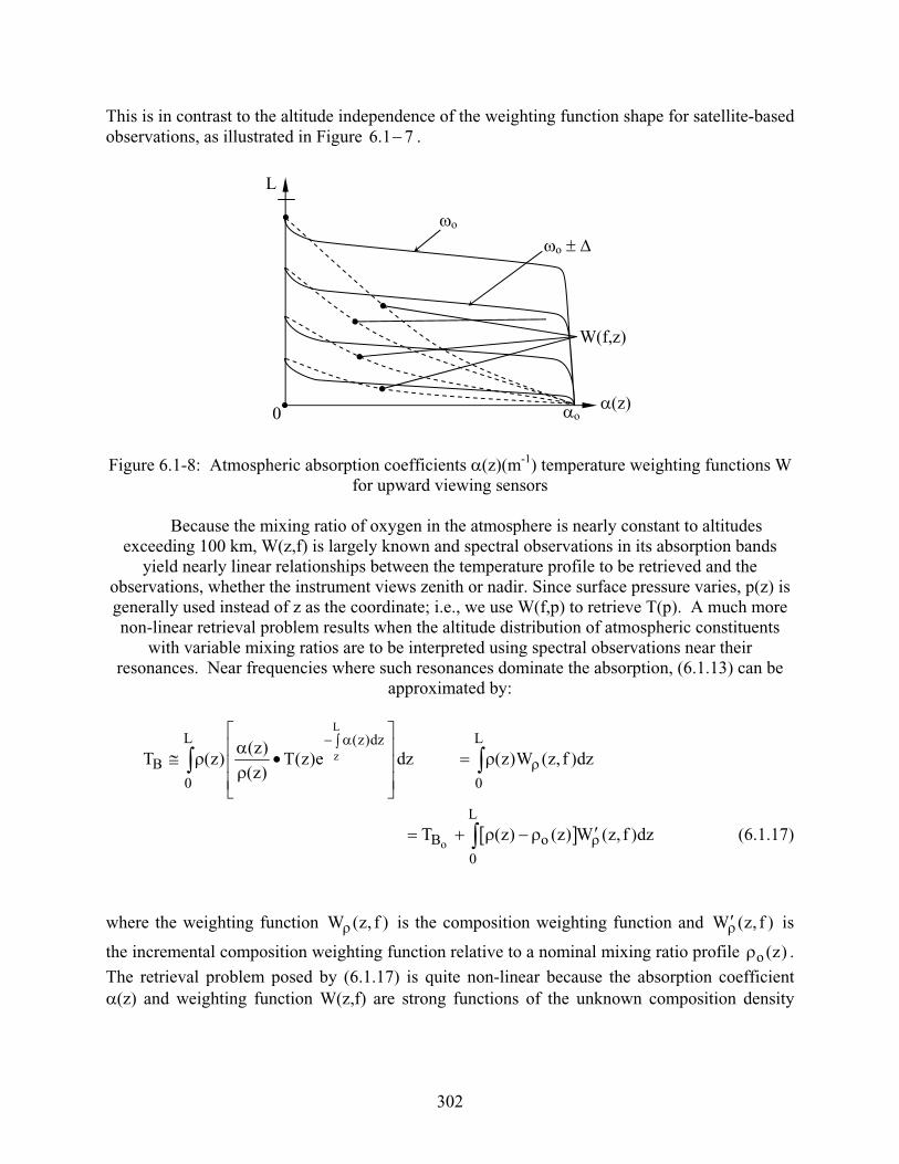
This is in contrast to the altitude independence of the weighting function shape for satellite-based observations, as illustrated in Figure 6.1 7 .

Figure 6.1-8: Atmospheric absorption coefficients (z)(m-1) temperature weighting functions W for upward viewing sensors

Because the mixing ratio of oxygen in the atmosphere is nearly constant to altitudes exceeding 100 km, W(z,f) is largely known and spectral observations in its absorption bands

yield nearly linear relationships between the temperature profile to be retrieved and the observations, whether the instrument views zenith or nadir. Since surface pressure varies, p(z) is generally used instead of z as the coordinate; i.e., we use W(f,p) to retrieve T(p). A much more non-linear retrieval problem results when the altitude distribution of atmospheric constituents

with variable mixing ratios are to be interpreted using spectral observations near their resonances. Near frequencies where such resonances dominate the absorption, (6.1.13) can be

approximated by:

L

z

o

L L(z)dz

B0 0

L

B o0

(z)T (z) T(z)e dz (z)W (z, f )dz

(z)

T (z) (z) W (z, f )dz (6.1.17)

where the weighting function )f,z(W is the composition weighting function and )f,z(W is

the incremental composition weighting function relative to a nominal mixing ratio profile )z(o .

The retrieval problem posed by (6.1.17) is quite non-linear because the absorption coefficient (z) and weighting function W(z,f) are strong functions of the unknown composition density

L

o

o

W(f,z)

(z)0 o

303

(z). In fact, the problem is singular if T(z) is constant, because the observed spectrum is then independent of the composition profile. As before, it can be helpful to use a priori statistics for (T(z), (z)) and incremental weighting functions W p(z,f) relative to a moderately accurately known reference profile )z(o .

6.1.4 Linear Least-Squares Estimates

Whether we are addressing nearly linear or highly non-linear problems, such as the moderately linear temperature profile retrieval problem of (6.1.13) or the much more non-linear composition profile retrieval problem posed by (6.1.17), we may nonetheless use linear retrievaltechniques, although with varying degrees of success. In fact, such linear techniques are frequently used for most estimation problems because of their simplicity and widely understood character. Perhaps the most widely used estimation technique is linear regression or multiple

regression, for which the estimated parameter vector p̂ is linearly related to the observed data

vector d by the determination matrix D :

dDp̂ (6.1.18)

The data vector often includes a constant as one element. For example, we may define the data vector as:

N1 d,...,d,1d (6.1.19)

where we have N observations, perhaps corresponding to N spectral channels.

Multiple regression employs that D which minimizes the mean square error of the estimate,

where the error for a single estimate is pp̂ . To derive D we may differentiate that mean

square error with respect to ijD and set it to zero. That is:

t

ij

tt tjj j i

ij

ˆ ˆE p p p p 0D

E d D p Dd p E 2d D d 2d pD

(6.1.20)

where iD is the thi row of D . Therefore:

304

j j i j

j j

t t

D E d d E p d

D E d d E p d

D E d d E p d

(6.1.21)

In terms of the data correlation matrix, t

dC E d d , (6.1.21) becomes:

t t tdC D E d p (6.1.22)

If the data correlation matrix dC is not singular, then we may solve for the optimum determination matrix:

t 1 t

dD C E d p (6.1.23)

Although D yields the minimum-square-error for a linear solution having the form (6.1.18), a linear estimator is optimum only under certain special assumptions: 1) the physics of the problem is linear such that:

npMd (6.1.24)

where the true parameter vector p is related to the data by the matrix M , and the data is

perturbed only by additive jointly-gaussian noise n , and 2) the parameter vector p is a jointly Gaussian process characterized by the probability of distribution:

mpmp

2

1

212Np

1t

e)2(

1pP (6.1.25)

where the parameter correlation matrix is non-singular and is defined as:

tt

mpmp E (6.1.26)

and where m is the expected or mean value of p .

305

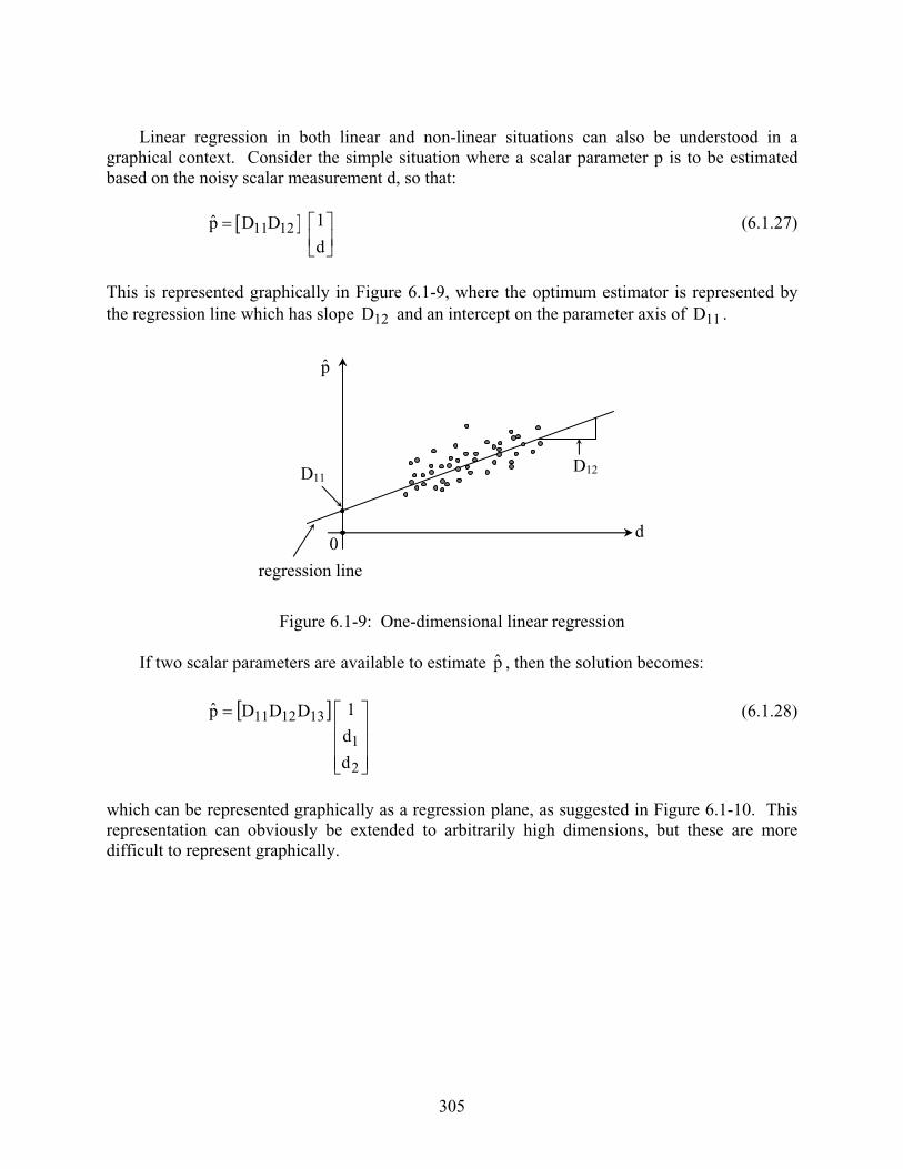
Linear regression in both linear and non-linear situations can also be understood in a graphical context. Consider the simple situation where a scalar parameter p is to be estimated based on the noisy scalar measurement d, so that:

11 12 1p̂ D Dd

(6.1.27)

This is represented graphically in Figure 6.1-9, where the optimum estimator is represented by the regression line which has slope 12D and an intercept on the parameter axis of 11D .

Figure 6.1-9: One-dimensional linear regression

If two scalar parameters are available to estimate p̂ , then the solution becomes:

2

1

131211

d

d

1DDDp̂ (6.1.28)

which can be represented graphically as a regression plane, as suggested in Figure 6.1-10. This representation can obviously be extended to arbitrarily high dimensions, but these are more difficult to represent graphically.

p̂

D11

0d

D12

regression line

306

Figure 6.1-10: Two dimensional regression

Often the linear regression (6.1.27) is expressed instead only in terms of 12D and the mean

values of the parameter and the data, < p > and < d >, so that ddDpp̂ 12 , as suggested

in Figure 6.1-11.

Figure 6.1-11: Linear regression with means segregated

It is shown below that linear regression estimates extract information in two ways: from the physics of the sensor via weighting functions, and from “uncovered” information to which the instrument is blind but which is correlated with information the instrument does see. A third category of information is “hidden” and is both unseen by the instrument and uncorrelated with any observable information; the hidden information is lost. If the statistical relevance of the data

used to derive the determination matrix D is considered marginal, then it is often useful to

p̂

0d

D12p

d

slope = D13

D11

p̂

d1

slope = D12

regressionplane

d2

307

discount this information accordingly. These two sources of information provided by physics and statistics can be separated, as follows.

To understand the nature of the information provided by the instrument without using statistics, consider the special case of noiseless data and linear physics where:

TWd (6.1.29)

where the data vector d is that of (6.1.19) and the parameter vector, for example, is the

temperature profile T . W is the weighting function matrix and iW is the thi row of W . It is shown below that if:

N

1iii WaT (6.1.30)

and W is not singular, then

TdDT̂ (6.1.31)

That is, if the unknown parameter vector is a linear combination of the weighting functions and the noise is zero, then that unknown vector can be retrieved exactly if the weighting function

matrix W is not singular.

To prove (6.1.31) we may begin by using the Gram-Schmidt procedure to define an orthonormal set of basis functions )h(i that characterizes the weighting functions:

1 11 1

2 21 1 22 2

3 31 1 32 2 33 3

W (h) b (h)

W (h) b (h) b (h)

W (h) b (h) b (h) b (h)

(6.1.32)

where:

j)=1(ior),ji(0dh)h()h(0

ijji (6.1.33)

308

Both i and ijb are known apriori if we restrict ourselves to the special case where the

parameter vector T(h) is a linear combination of the weighting functions; then:

N

1iii )h(Wk)h(T (6.1.34)

0

jj dh)h(W)h(Td (6.1.35)

Substituting (6.1.34) into (6.1.35) yields:

N

1i 0jiij dh)h(W)h(Wkd

N

1iiji

N

1i 0

ij

1nnjn

i

1mmimi Qkdh)h(b)h(bk (6.1.36)

Therefore;

kQd (6.1.37)

and we may solve for k exactly if the known square matrix Q is non-singular. The exact

parameter vector T(h) can then be retrieved by substituting the solution for k from (6.1.37) into (6.1.34).

It is useful to combine (6.1.34) with the solution to (6.1.37) to yield:

dDdQWdQWkWT11

(6.1.38)

where we define the resulting D as the minimum information solution, for which:

1

QWD (6.1.39)

The minimum information solution is therefore exact for the noiseless case where the unknown parameter vector T is any linear combination of the weighting functions, so the claim is proved.

309

One of the principal benefits of linear regression is that additional information is extracted from apriori statistics. By virtue of (6.1.35) an instrument yields no response, or is “blind”, to any component of the parameter vector T(h) which is orthogonal to the space spanned by the available set of weighting functions )h(Wj , which is the space spanned by )h(i for 1 i N,

where N is the number of weighting functions. In general, the parameter vector T(h) is the sum of components which are “seen” by the instrument plus all hidden components:

1Ni

iiN

1iii )h(a)h(Wk)h(T (6.1.40)

Consider the extreme case where )h(1 is always accompanied by 0.5 )h(1N . Then the

minimum information solution could be improved using:

N

2iii1N11 a5.0a)h(T̂ (6.1.41)

The factor 0.5 would shrink to the degree that )h(1 became decorrelated with )h(1N . By

extension, the multiple regression estimator becomes:

1Nj

jiji

1i aQWD wheredDT̂ (6.1.42)

The first term in the expression for iD is the minimum information solution and the second term is the uncovered information which we might define as the function i . Thus the retrieval can

be drawn only from the space spanned by N1N1 ,...;,... . That is, the solution space can be

spanned by 2N functions, but because of the fixed relationship between i and i , the dimensionality remains N. Thus N channels contribute N orthogonal basis functions to the minimum-information solution, plus N more orthogonal basis functions which are statistically correlated with the first N. As N increases, the fraction of the hidden space which is spanned by

)N,...,1i(i and “uncovered” by statistics is therefore likely to increase, even as the hidden space shrinks. In general, the apriori variance equals the sum of the observed, uncovered, and lost variance (lost due to noise and decorrelation).

As an example of the advantages of having more independent observations when statistics are used, consider eight channels of the AMSU atmospheric temperature sounding instrument versus its four-channel MSU predecessor. Both these instruments are passive microwave spectrometers in earth orbit sounding atmospheric temperature profiles with ~10 km weighting functions peaking at altitudes ranging from 3 to 26 km. Figure 6.1-12 illustrates how the total apriori variance in the ensemble of temperature profiles studied is divided between the variances seen, uncovered, and lost by these two instruments. The sum of these three components is

310

always the same and represents the sum of the a priori variances for the 15 levels in the atmosphere used between 0 and 30 km; this total over the 15 levels was 1222 K2 for a mid-latitude ensemble, and 184 K2 for a tropical ensemble. Note that for both 55 and nadir incidence angles the ratio between lost and uncovered power for MSU is approximately 0.7. Although AMSU observes directly with the minimum information solution a much larger fraction of the total variance, roughly 90 percent, nonetheless the fraction of the variance uncovered by statistics is now greater than for MSU and the ratio between lost and uncovered power is only ~0.4.

Figure 6.1-12 : Relative importance of physics and statistics in recovering information in multiple regression; MSU and AMSU employ 4 and 8 channels, respectively.

That is, by using more channels, statistics was able to recover a larger fraction of that variance which was unobservable by the instrument. The same significant advantage of using more channels was even more evident in the tropical example.

MID-LATITUDES (TOTAL POWER = 1222 K2, 15 LEVELS)

OBSERVED POWER UNCOVERED POWER LOST POWER

MSU - 55 ANGLE, LAND

MSU - 0 ANGLE, NADIR

AMSU - NADIR

AMSU - NADIR3 km WEIGHTING FUNCTION 10 16 6 12 22 26

WINDOWTROPICS (TOTAL POWER = 184 K2)

MSU – NADIR, LAND

AMSU - NADIR

UNCOVER LOST

10 20 30 40 50 60 70 80 90 100

311

6.1.5 Principal Component Analysis

Unfortunately multiple regression yields inferior results when the number of training

samples from which the determination matrix D is derived is too limited. Sometimes this limit is imposed by economics and sometimes by a desire to use only recent or nearby training data when estimating the next retrievals. Fortunately a powerful technique can often significantly reduce these errors due to limited training samples. This method, sometimes called principal component regression (PCR), filters the data vectors before performing the regression, where this filtering is performed by determining a limited number of principal components, (PC’s) which are equivalent to the eigenvectors in the Karhunen-Loeve transform (KLT), or to empirical orthogonal functions (EOF). The orthonormal basis functions for the KLT are the columns of a

square matrix K and are the eigenvectors of the data correlation matrix ddC , where:

t

dd dd EC (6.1.43)

The first eigenfunction 1iK is that which most closely represents the ensemble of possible data

vectors, and therefore typically resembles the ensemble average of d . The second eigenvector

2iK is that function which most effectively reduces the residual variance over the ensemble,

given the amplitude of the first eigenvector. That is, the KLT matrix K transforms the data vector to a new vector:

i j ij i

d K d

E d ' d ' (6.1.44)

where i are the eigenvalues of the matrix ddC arranged in declining order. Equivalently:

K

0

0

KC

n

2

1tdd (6.1.45)

Principal component analysis (PCA) can sometimes be improved significantly by reducing the effects of additive noise when that noise differs significantly from variable to variable. Consider the generalization of the noiseless case (6.1.29) to the case where there is additive gaussian noise so that the available data vectors can be represented as:

nGTWd21

(6.1.46)

312

where W is the known mixing matrix and T is the parameter vector arising from a stochastic

process characterized by a covariance matrix of order p. G is the unknown diagonal noise covariance matrix and the noise vector n is assumed to be gaussian with zero mean and to have a correlation matrix which is the identity matrix of order m. It can be shown that if the data vector for which PCA is to be performed is first normalized to yield

dGd21

na (6.1.47)

then the resulting analysis is more faithful to the underlying process; nad is called the noise-adjusted data. The variance of the additive noise in noise-adjusted data is identical across all variables. Without noise adjustment PCA tends to emphasize the influence of parameters with larger noise vectors; this problem is more severe when the data set used for PCA is limited in size so that the noise contributions cannot be reduced by averaging. The resulting principal components for the data set nad are called noise adjusted principal components (NAPC).

Thus an important way to improve multiple regression estimators (6.1.18) and (6.1.23), is to

replace d with nad when computing 1dC and

tpdE in (6.1.23).

These regressions can be improved still further by using principal components regression (PCR) in noisy circumstances when the training data set is limited. PCR uses only a subset of the PC’s d (6.1.44) to perform the regressions, the lower order terms being too noisy. Various

methods exist for determining how many elements m of d should be retained, but this number

m generally does not exceed the rank of the noise-free data vector d . One approach to determining this cut-off m is to employ a scree plot of the logarithms of the eigenvalues i

versus i. These logarithms typically decline steeply with i until they approach an asymptote representing the noise floor of the ensemble; values of i corresponding to this floor contribute primarily noise and generally should not be included in PCR.

Methods approaching NAPC in performance and generally exceeding that of PCR have

been developed for cases where the signal order (rank of W in (6.1.45)) and noise variances Gare unknown. These include blind-adjusted principal components (BAPC) and blind principal component regression (BPCR). This approach iteratively estimates the order of the random process and then the noise variances. Improvements over PCR are greatest when the 1) number of variables in d is large 2) the training set is limited, and 3) the noise on the various data elements varies substantially in an unknown way. This method has been described by Lee and Staelin (Iterative Signal-Order and Noise Estimation for Multivariate Data, Electronics Letters,37, 2, pp 134-5, January 18, 2001) and Lee (PhD thesis, MIT, EECS, March 2000).

313

6.2 NON-LINEAR ESTIMATION

6.2.1 Origins of Non-linearity

Non-linear estimation techniques are generally superior to linear methods when the

relationship between the observed and desired parameters is non-linear, or when the statistics

characterizing the problem are non-jointly-gaussian. A simple illustration of the superiority of

non-linear estimators is provided in Figure 6.2-1, which characterizes the non-linear physical

relationship between the desired parameter p and the available data d in terms of a scatter

diagram representing the outcomes of multiple experiments.

D2 slope

d

data

best fit,"linear regression"

pparameter

Optimum estimator

D1

p(d)^

P{p}

0p

probabilitydistribution

a)

b)

Figure 6.2-1: a) Best-fit linear regression line for a finite set of training data characterizing a

non-linear physical relationship between the desired parameter p and observed data d; b)

probability distribution P(p) characterizing the training set

The linear regression best fit is given by:

314

d

1DDp̂ 21 (6.2.1)

where the scalars 1D and 2D represent the baseline intercept and the slope of the best-fit linear regression, respectfully. It is clear from the figure that the optimum estimator is a curved line, as illustrated, rather than the linear regression. It is also clear that the probability distribution applicable when the measurement is made should be similar to that of the training data, which is that finite set of data used when the best-fit linear regression was computed. If the probability distribution of the training data differs from that of a test ensemble of data, the test estimates will be biased accordingly.

A simple illustration of how non-gaussian statistics can lead to an optimum non-linear estimator is shown in Figure 6.2-2.

Figure 6.2-2: a) Best linear and non-linear estimator for a linear, but non-gaussian set of training data, b) MAP and MSE estimates for a given observation Ad

The physics illustrated by the training set of data points illustrated in Figure 6.2-2 is linear but non-gaussian, which can result in negative values for p being estimated for this training set, even though negative values of p never occur. A non-linear estimator can avoid this problem, as illustrated. Figure 6.2-2b shows the a posteriori probability distribution AdpP . The maximum

a posteriori probability “MAP” estimator, by definition, selects the maximum point on this

Adp̂

Ad

Adp̂(a)

0

best non-linear estimator (avoid 0p̂ )

p

d

Maximum aposteriori Probability “MAP” estimator

AP p d

Adp̂MSE

(b)

(linear)

(non-linear)

non-linearp

315

distribution, which is at p = 0 here. The minimum-square-error estimator Adp̂ is located near

the center of gravity of the probability distribution and minimizes the mean square error given

Ad . To the extent a smooth probability distribution AdpP can be defined for the training set,

the MSE non-linear estimator is easily found. The MAP estimator would approximate the best linear estimator for larger values of p, and would be pinned at 0p̂ only when p 0. Note that this MSE estimator is non-linear because the statistics are non-gaussian, even though the physics itself is linear.

Non-linear estimators can be constructed in many ways. They might be simple polynomials, spline functions, trigonometric functions, or the outputs of neural networks. Recursive linear estimators can also be employed, as described in Section 6.2.3.

6.2.2 Perfect Linear Estimators for Certain Non-linear Problems

There exists certain non-linear problems for which linear estimators can be used with perfection. Consider the case where a single parameter p is to be estimated based on two observed pieces of data, 1d and 2d , where

221o1 papaad (6.2.1)

221o2 pbpbbd (6.2.2)

For this example we assume the data is noiseless. It follows from (6.2.2.) and (6.2.1) that

21o22 bpbbdp (6.2.3)

221o21o221o1 dcpccbpbbdapaad (6.2.4)

Note that (6.2.4) defines a plane in the three-dimensional space 21 d,d,p . This plane defines a perfect solution

1221o cdcdcpp̂ (6.2.5)

Where the constant 1c must be non-zero and is

2 11 1

2

a bc a

b (6.2.6)

Thus a linear estimator yields a perfect answer even though the relationship between the unknown parameter p and the two observed data points 1d and 2d is non-linear. The graphical

316

representation in Figure 6.2-3 suggests how this might be so. Figure 6.2-3 illustrates the case where the non-linear relationship between p and 1d effectively cancels the non-linearities in the

relationship between p and 2d so as to produce a net dependency 21 d,dp that is non-linear in

one dimension but lies wholly within the linear plane 21 d,dp̂ .

Figure 6.2-3: Linear-relationship plane for a non-linear estimation problem

This first example involved two observations 1d and 2d , and second-order polynomials in

p, as defined in (6.2.1) and (6.2.2). This example can be generalized to thn -order non-linearities. Let:

2nn

22n1nnn

nn2

2222122

nn1

2121111

pa...papacd

pa...papacd

pa...papacd

(6.2.7)

Where n21 d,...,d,d are observed noise-free data that are related to p by thn -order polynomials and all aij are known. Note that the number n of independent observations for the single parameter p at least equals the order of the polynomial relating id and p. We can show that in non-singular cases there exists an exact linear estimator

constantdDp̂ (6.2.8)

d2

d1

p p(d2,d1)

d2 = f2(p)

plane p̂ (d1,d2)is the linear

d1 = f1(p)

plane p̂ (d1,d2) has two angular degrees of freedom to use for

minimizing p

317

To prove (6.2.8) let 1k1 and we can see from (6.2.7) that

n

1iini

nn

1i1ii

n

1iii

n

1iii akp...akpckdk (6.2.9)

The other n-1 constants ik remain undefined for 2i . To solve for these unknowns we create

n-1 equations that set the higher-order terms (n 2) in (6.2.9) to zero:

0akn

1iiji for j = 2,3,…,n (6.2.10)

Therefore,

n

i ij 1ji 2

k a a for j = 2,3,…,n (6.2.11)

If we define the (n –1) element vector s as

12 13 1ns -a , a ,..., a (6.2.12)

then:

1t

k 1, A s (6.2.13)

where ijA a for i,j = 2,3,…,n.

Therefore

n

1i

n

1i1iiiii akcdkp (6.2.14)

which is a linear function of d and can be computed if A is not singular, and if

n

1i1ii 0ak (6.2.15)

318

Therefore we have proven that the parameter p can be expressed as a linear function of d , even though each measurement id is related to p by a different polynomial, provided that the order of

the polynomial n is equal to or less than the number of different observations, and the matrix Ais not singular.

6.2.3: Non-linear Estimators

Non-linear estimation is a major area of current research. In this section six of the more common methods are briefly illustrated. These methods include: 1) iterated linear estimates, 2) computed MAP and MSE estimators, 3) MSE estimators operating on data vectors augmented by simple polynomials or other non-linear functions, 4) same as method (3), but with rank reduction of the augmented data vector, 5) neural networks, and 6) genetic algorithms.

Iterated linear algorithms are best understood by referring to Figure 6.2-1, where it is clear that a single linear estimator will be non-optimum if we know that the desired parameter is in a region where the linear estimator is biased; for example, this estimator is biased at the two ends of the distribution and in the middle. If, however, the first linear estimate of the desired parameter p is followed by a second linear estimator which is conditioned on a revised probability distribution P{p}much more narrowly focused on a limited range of p, then the second estimate should be much better. This process can be iterated more than once, particularly if the random noise is small compared to the bias introduced by the problem non-linearities.

In some applications these iterations are computationally burdensome. In such cases, if the parameter being estimated changes slowly from sample to sample, the first guess for each new estimate can be obtained from the previous estimate. If the two consecutive samples are very similar, which is frequently the case, then one or two iterations should suffice, reducing the computational burden that would be imposed if a less accurate first guess were used. If the first guess yields a predicted data vector that departs substantially from the observed data, then a default first guess might be used instead.

An example of a non-linear MAP estimator is shown in Figure 6.2-2b. The same figure also illustrates how a non-linear MSE estimator could be computed.

Mildly non-linear estimators can also be found by using

augdDp̂ (6.2.16)

where augd is the original data vector augmented with simple polynomials, trigonometric

functions, or other non-linear elements which efficiently represent the kind of non-linearity

desired. The determination matrix D is computed using (6.1.23). One difficulty with this

technique is that the resulting data correlation matrix dC is often nearly singular and the estimates may be unsatisfactory.

319

In this nearly singular case it is useful to reduce the rank dC first using the KLT or the equivalent PCA, as discussed in section 6.1.5. Rank reduction can be used to reduce the dimension of the original unaugmented data vector d or the dimension of the augmented data

vector augd , or both. In either case those eigenvectors with small eigenvalues, and therefore

poor signal-to-noise ratios, are dropped from the process. This noise reduction step is more efficient if the KLT or PCA is performed after the variables are noise normalized so that the additive noise variance is approximately equal across variables.

Arithmetic neural networks, modeled in part after biological neural networks, compute complex polynomials with great efficiency and simplicity, and provide a means for matching the polynomials to given training ensembles so as to minimize mean-square estimation error. Figure 6.2-4 illustrates how a single layer of a simple neural network might be constructed.

Figure 6.2-4: Single layer of a feed-forward neural network

This network operates on N input data values id to produce M outputs 'id which are non-linearly

related to the inputs. N can be larger or smaller than M. The network first multiplies each data value di by a constant ijW before these products are separately summed to produce M linearly

related outputs, which then pass through a sigmoid operator to yield the non-linear outputs 'id .

Usually the sigmoid operators are omitted from the final layer. One common sigmoid operator is xtanh'd where x is the input to the sigmoid operator. One of the network inputs is the

constant unity, which permits each of the sums to be biased into the convex, linear, or concave portions of the sigmoid operator, depending on what type of non-linearity is desired. If the gains are sufficiently large, the sigmoid approaches a step function in the limit, where it acts like a logic gate. Such single-layer neural networks can be cascaded, as suggested in Figure 6.2-5, where the last layer of the system estimates the desired parameter vector p̂ .

1

d1

dN

1

M

W01

W11

WN1

d 1

d M

320

Figure 6.2.5: Multi-layer neural network with two hidden layers

The most popular technique for determining the weights ijW for a set of training data is the

back-propagation algorithm, which has many variations, and about which books have been written. The success and popularity of neural network techniques has lead to commerically available computer tool kits which make them easy to apply to practical problems. In general the networks are trained for given ensembles of data and then applied to larger data sets. Because neural networks have large numbers of degrees of freedom, i.e., the number of weights is large, it is important that the number of independent training examples be substantially larger so as to produce a robust result. Otherwise the network can be “overtrained” resulting in the estimator slavishly duplicating the training outputs at the expense of accuracy for the larger data set. For this reason, training is often stopped when an independent set of “test” estimators, not part of the training set, suggest that this error has ceased declining and is beginning to grow. It is good practice for the degrees of freedom in the training data set to exceed the number of weights by a factor of three or more.

The more highly non-linear problems generally need more network layers and more internal hidden nodes, where the optimum number of layers and hidden nodes is generally determined empirically for each task. Neural networks can be used not only for estimation, but also for recognition and category identification.

For complex problems it is generally best to minimize the degrees of freedom in the neural network and to blend it with linear systems which are intrinsically more stable. For example, a neural network is often preceded by normalization of the variables so that they all exhibit comparable noise variances. Then a KLT can rotate their noise-normalized input vector prior to a truncation that preserves only those transformed variables with useful signal-to-noise ratios. Current practice generally involves substantial empirical trial and error in selecting the type of neural network numbers (numbers of nodes and layers) and type of optimization to be employed on any particular problem.

Genetic algorithms can be combined with any of the foregoing strategies, provided the algorithm can be represented by a segmented character string such as a binary number. For example, this numerical string can represent an impulse response that defines a matched filter. It may also represent the weights in a linear estimator or neural network, or could characterize the architecture of a neural network, e.g., the number of layers and number of nodes per layer. Although one could test the performance of all possible character strings, and therefore all

d 1NN 2NN 3NN p̂'d ''d

“hidden layers”

321

possible algorithms, and choose the best, the genetic algorithm permits this trial-and-error procedure to be executed much more efficiently.

Generally all competing algorithms are represented by character strings of the same length, where each position along these strings has a defined significance that is the same for all strings. Many strings are then tested and the better ones are identified. Elements from the better ones are then randomly combined (“genetically”) in the proper sequence to form new complete strings (and algorithms); some random mutations may also be added. Then more testing occurs with multiple competing members of the new generation of algorithms, and the evaluation and selection process is repeated. Thus algorithm elements compete in a “survival of the fittest” test. Eventually an asymptotic optimum may be approached. In general, the estimators produced by genetic algorithms or neural networks are not perfect, and so several solutions are typically produced before the best is selected.

In any of these algorithms there is some opportunity to redefine the input data vector to include some of its spatial or chronological neighbors. In cases where adjacent data vectors are statistically related, this can produce superior results. Unfortunately the dimensionality of the problem often increases unacceptably rather quickly as such neighbors are included. In this case it is important to employ efficient data compression techniques that preserve the more important information-bearing elements of the adjacent data vectors, while excluding the rest. Kalman filtering is an example of such efficient use of adjacent or prior data in the estimation of a current parameter vector.