119

CHAPTER 6

HARDWARE IMPLEMENTATION

6.1 INTRODUCTION

Hardware implementation is done using an actual machine to verify

the effectiveness of the linearization technique proposed. TMS320F2812 DSP

controller operating with a clock speed of 150 MHz was used to carry out the

implementation. In this chapter, description of the hardware, flowchart of

control, experimental results and discussion are given.

6.2 DESCRIPTION OF HARDWARE

6.2.1 Permanent Magnet Synchronous Motor

Surface Mounted Permanent Magnet motor is used for the hardware

implementation. This configuration is used for low speed applications because

the magnets will fly apart during high speed operations because of the

lamination. These motors are considered to have small saliency, thus having

practically equal inductances in both axes ).The rotor has an iron

core that may be solid or may be made of punched laminations for simplicity

in manufacturing. Thin permanent magnets are mounted on the surface of this

core using adhesives. The construction and applications of this motor are

given in detail in Bose (2002).

120

Motor Specifications

Nominal Operating Voltage (Vd) = 325V

Continuous stall torque (Mo) = 2.2 Nm

Continuous stall current (Io) = 3.69 A

Peak stall Torque (Nmax) = 6.60 Nm

Peak stall current (Imax) = 11.1A

Rated Torque (Mn) = 2.2 Nm

Rated Current (In) = 3.69A

Rated Power (Pn) = 1.1 hp

Rated Speed (Nn) = 4600 rpm

Torque Constant (Kt) = 0.6 Nm/Arms

Terminal to terminal Resistance (Rtt) = 3.07

Terminal to terminal Inductance (Ltt) = 6.57 mH

Moment of Inertia w/o brake (J) = 1.28 kg

Weight w/o brake (M) =4.2 kg

6.2.2 TMS320F2812 DSP

TMS320F2812 DSP controller is a programmable digital controller.

The controller combines the power CPU with the on-chip memory and the

peripherals. The Controller offers 60 MIPS (million instructions per second)

performance. This fast performance is well suited for processing control

parameter in application where large number of calculation are to be

computed quickly. The architecture of TMS320F2812 CPU, components of

CPU, Event Manager, Analog to Digital Converter (ADC) are all referred

from Manuals of TMS320F2812 DSP controllers

(http://www.ti.com/product/tms320f2812).

121

The event manager is the most important peripheral in digital motor

control. It supports the functions needed for controlling the electromechanical

device. There are two identical Event Managers (EVA and EVB) on

TMS320F2812. Each event manager module of TMS320F2812 contains

several sub components such as Interrupt logic, General-Purpose (GP)

Timers, Full- Compare Unit, Programmable Deadband Generator, PWM

Waveform Generation, Double Update PWM Mode, Capture Unit,

Quadrature - Encoder Pulse (QEP) Circuit, GP Timer, Compare Unit, Capture

Unit and Quadrature Encoder Pulse Unit.

The ADC module has 16 channels, configurable as two

independent 8-channel modules to service event managers A and B. The two

independent 8-channel modules can be cascaded to form a 16-channel

module. Although there are multiple input channels and two sequencers, there

is only one converter in the ADC module. Functions of the ADC module

include 12-bit ADC core with built-in dual sample-and-hold (S/H),

simultaneous sampling or sequential sampling modes, Analog input: 0 V to 3

V , fast conversion time (runs at 25 MHz ADC clock or 12.5 MSPS), 16-

channel, multiplexed inputs and auto sequencing capability providing up to 16

“auto conversions” in a single session. Each conversion can be programmed

to select any 1 of 16 input channels. Sequencer can be operated as two

independent 8-state sequencers or as one large 16-state sequencer (i.e., two

cascaded 8-state sequencers). Sixteen result registers (individually

addressable) store conversion values.

6.2.3 Intelligent Power Module (IPM)

IPM based power module works as a DC-DC Converter (Chopper)

or DC-AC Converter (Inverter). It works using a IGBT based IPM and works

122

on the basis of software from DSP Processor. The power module can be used

for studying the operation of chopper, three phase inverter, single phase

inverter and speed control of three phase induction motor and single phase

induction motor.

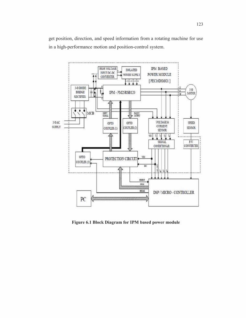
The block diagram of IPM Based Power Module (PEC16DSMOl)

is shown in Figure 6.1 http://www.ti.com/product/tms320f2812). It consists

of

1. Intelligent Power Module

2. Voltage and Current Sensor

3. Signal Conditioner

4. Protection Circuit

5. Opto Coupler

6. 3 diode bridge Rectifier

7. Speed Sensor

8. Frequency to voltage converter

Intelligent Power Modules are advanced hybrid power devices that

combine high speed, low loss IGBTs with optimized gate drive and

protection circuitry. Highly effective over-current and short-circuit protection

is realized through the use of advanced current sense IGBT chips that allow

continuous monitoring of power device current. The system reliability is

further enhanced by the IPM's integrated over temperature and under voltage

lock out protection. The enhanced quadrature encoder pulse (eQEP) module

is used for direct interface with a linear or rotary incremental encoder

123

get position, direction, and speed information from a rotating machine for use

in a high-performance motion and position-control system.

Figure 6.1 Block Diagram for IPM based power module

124

6.3 IMPLEMENTATION

Figure 6.2 Hardware Implementation Diagram

The proposed system of Figure 6.2 was implemented.

TMS320F2812 DSP controller operating with a clock speed of 150 MHz was

used to carry out the implementation of Clarke’s and inverse Clarke’s

transformation, Park’s and inverse Park's transformation (Toliyat and

Campbell 2003), linearizing transformation, PI controller, inverter switching

for speed control. Also estimation of rotor position and speed are carried out

with the help of the pulses obtained from the speed encoder. A three phase

insulated gate bipolar transistor (IGBT) intelligent power module is used for

the inverter, which is supplied at a DC link supply voltage of 325 V. An

incremental encoder (@2000 pulses/rev) is used to calculate the rotor speed

and to determine the initial position of rotor position ( ).

125

Procedure for implementation can be followed as given. The power

supply of controller, converter, and auto transformer is switched ON. The

programme is loaded to the processor by using the Code Composer Studio

(CCS) software and the pulses in the CRO is checked. If the pulses are

appropriate, the MCB of converter is switched ON and voltage is applied

using auto transformer to the full voltage. The input ac voltage is converted to

dc voltage using the rectifier section. The capacitor (1000 f) in the circuit is

used to reduce ripple in the dc voltage. The DC voltage is given as input to

the inverter section. The output voltage of the inverter is fed to the motor and

it starts rotating. The speed of the motor is controlled by using the processor

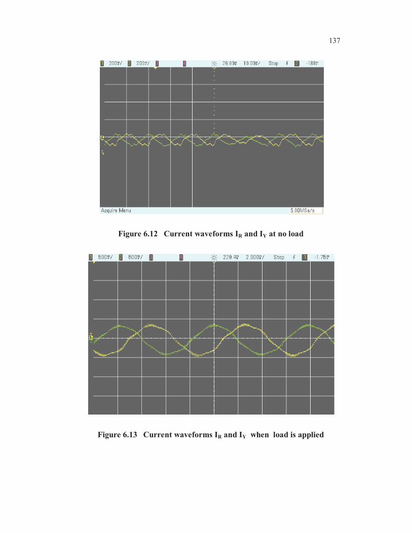
by varying the reference speed. The required output waveforms (voltage ,

currents ) can be observed using isolated port in the converter.

6.3.1 Estimation of Rotor Position and Speed

The initial position of the rotor ) is known from the index pulse

which is obtained from the speed encoder and some fixed duty cycle is given

to the inverter switches. The speed and rotor position values are calculated

using the following procedure:

(i) The encoder pulse gives 2000 pulses per single rotation from

the motor.

(ii) The number of electrical cycles to be generated for a single

mechanical rotation is equal to the number of pole pairs. Here

number of pole pairs=2, so two electrical cycles should be

generated for one mechanical rotation.

(iii) So for every 1000 pulses from the encoder, one electrical

cycle should be generated so rotor position varies from 0 to

126

3600 where the number of pulses from encoder varies from 0

to 1000.

So = Number of pulses generated × 360/1000

(iv) Speed is estimated by calculating the time period of single

pulse obtained from the encoder pulse of speed encoder in the

motor.

(v) The timer is ON when one rising edge of encoder pulse occurs

and timer is turned off when the next rising edge occurs.

(vi) This value of the timer count is calculated for a fixed speed

(i.e. 4600 RPM) and the count is used for estimating all the

speeds.

Speed = (4600 × Timer count for 4600rpm speed) / Timer

count for the present speed

6.3.2 PWM Generation

Initially PWM comparative registers are loaded with some fixed

value. With the help of rotor position value which is calculated from

encoder pulse, three sine waves are generated and fed to the PWM

comparative registers. So, based on required speed, the PWM is updated.

6.4 SPEED CONTROL BEFORE LINEARIZATION

Speed control of PMSM is implemented using PI controller. The

line currents obtained from the inverter are converted into 2-phase stationary

currents using Clarke’s transformation. Using Park’s transformation, the same

are converted into 2- phase rotationary currents and . The actual speed

and the reference speed are compared and the error is fed to PI controller. The

127

outputs of the PI controller are converted to 2-phase stationary currents and

later to three phase currents and using Inverse Park’s and Inverse

Clarke’s transformation. and are quantified and loaded into

comparative registers to get the required PWM pulses.

6.4.1 Calculation of rotor position

The speed encoder gives index pulse and encoder pulse. When

index pulse is received, is initialized. The encoder pulse gives 2000 pulses

for a single rotation of rotor. Within the 2000 pulses received, two electrical

cycles are generated. Number of pulses are counted and is calculated based

on the count, to generate sine wave of required frequency. Using the same

encoder pulse, speed is calculated.

6.4.2 Implementation of Clarke’s Transformation

The two line currents and obtained from the inverter output

are read and converted into 2- stationary currents using the formula

(6.1)

=1

1.732( + 2 ) (6.2)

6.4.3 Implementation of Park’s Transformation

2- stationary currents and are converted into 2- rotationary

currents and by using the formula

= (6.3)

128

= (6.4)

Here and are calculated using the theta value calculated

from the encoder pulse.

6.4.4 PI Controller

The actual speed is compared with set speed and the error is given

to the speed PI controller. The output of speed PI controller is given as

reference for PI controller. is compared with reference (zero) and the

error is given to the PI controller.

6.4.5 Inverse Park’s Transformation

The outputs of PI controller and PI controller are converted

into 2- stationary currents using the formula

= (6.5)

= (6.6)

6.4.6 Inverse Clarke’s Transformation

The 2- stationary currents are converted in to 3- currents using

the formula.

(6.7)

1

21.732 (6.8)

1

2+ 1.732 (6.9)

129

and are quantified and loaded into compare registers to get the

required PWM pulses.

6.5 SPEED CONTROL OF PMSM AFTER LINEARIZATION

The linearizing transformations as given in Equations (3.4) and

(3.5) are implemented.

The outputs of PI controllers, rotor position and rotor speed are

given as inputs to the linearizing transformations. The transformed state

variables after linearization are and transformed input variables

are . The linearizing transformations after scaling are given below

(Refer Figure 4.11 ).

and transformations

= 0.0000073 (6.10)

0.0000073 (6.11)

0.00657 (6.12)

( 0.00214) (6.13)

transformation

= Output of PI controller – (1158000 ) (6.14)

= Output of PI controller +(377000 ) (6.15)

130

transformation

PI controller output after linearization is = + (264409

) + (467 ) (6.16)

PI controller output after linearization is = (-3.069*

(1434 ) (6.17)

6.5.1 Inverse Park’s Transformation

The outputs of PI controller and PI controller after linearization are

converted into 2- stationary currents using the formula

= (6.18)

= (6.19)

6.5.2 Inverse Clarke’s Transformation

The 2- stationary currents after linearization are converted in to

3- currents using the formula.

(6.20)

1

21.732 (6.21)

1

2+ 1.732 (6.22)

and are quantified and loaded into compare registers to get

the required PWM pulses.

131

6.6 FLOW CHART

Flowchart for speed control after linearization is given in Figure

6.3.

Figure 6.3 Flowchart for speed control after linearization

6.7 EXPERIMENTAL RESULTS AND INFERENCE

Figures 6.4 and 6.5 show the dynamic responses of speed of the

drive system with respect to step change in speed reference from 250 to 2000

r/min and 250 to 3000 r/min respectively before linearization. The motor is

START

Duty cycle for generating PWM

pulses to be initialized/updated

Rotor angle, speed and currents to

be estimated using encoder output

Clarke’s and Park’s transformations

to be implemented

PI controller implementation

Linearization algorithm to be

implemented

Inverse Park’s and Clarke’s

transformation to be implemented

Duty cycle for PWM pulses to be

generated

132

driven at a load of 3 kg. Figures 6.6 and 6.7 show the dynamic responses of

speed of the drive system with respect to step change in speed reference from

250 to 2000 r/min and 250 to 3000 r/min respectively after linearization.

Figures 6.8 and 6.9 show the dynamic response of speed with respect to load

variations before linearization. Figure 6.8 shows the dynamic response of

speed when the set speed is 1500 r/min and when 1 kg load is applied. Figure

6.9 shows the dynamic response of speed when the set speed is 1500 r/min

and when 1 kg load is released. Figure 6.10 shows the dynamic response of

speed when the set speed is 1500 r/min and when 1 kg load is applied after

linearization. Figure 6.11 shows the dynamic response of speed when the set

speed is 1500 r/min and when 1 kg load is released after linearization.

It is seen from these figures that the dynamic responses of speed for

step change in speed reference is smoother and more uniform for cases after

linearization, when compared to the cases before linearization. Also it is seen

that there are spikes in the responses before linearization. The dynamic

responses of speed for load variations is also better for cases after

linearization, when compared to the cases before linearization. Hence it is

verified by experimental results that a better dynamic response under a fixed

controller can be obtained for the linearized system for variations of

reference speed and load conditions, in contrast to the case before

linearization.

Figures 6.12 and 6.13 show the current waveforms at no load and

loaded conditions respectively. Figures 6.14 and 6.15 show the pulse width

modulated VRY waveform and pulse width modulated waveforms after

filtering. Figures 6.16 and 6.17 show the pictures of the DSP controller used

for the control of PMSM.

133

Figure 6.4 Speed control before linearization when load is 3 kg and set

speed is 2000 rpm

Figure 6.5 Speed control before linearization when load is 3 kg and set

speed is 3000 rpm

134

Figure 6.6 Speed control after linearization when load is 3 kg and set

speed is 2000 rpm

Figure 6.7 Speed control after linearization when load is 3 kg and set

speed is 3000 rpm

135

Figure 6.8 Speed control before linearization when speed is 1500 rpm

and 1 kg is applied

Figure 6.9 Speed control before linearization when speed is 1500 rpm

and 1 kg is released

136

Figure 6.10 Speed control after linearization when speed is 1500 rpm

and 1 kg is applied

Figure 6.11 Speed control after linearization when speed is 1500 rpm

and 1 kg is released

137

Figure 6.12 Current waveforms IR and IY at no load

Figure 6.13 Current waveforms IR and IY when load is applied

138

Figure 6.14 Pulse width modulated VRY signal

Figure 6.15 Pulse width modulated signals 1 and 3 after filtering with

120o phase shift

139

Figure 6.16 Photograph 1 of DSP controller for PMSM

140

Figure 6.17 Photograph 2 of DSP controller for PMSM

6.8 SUMMARY

The implementation aspect of the controller for PMSM based on

linearization is discussed. The experimental results verify that a uniform

response is obtained for the linearized system for variations of reference

speed and load conditions, in contrast to the case before linearization. Thus

the experimental results verify the theoretical analysis and the effectiveness of

the proposed control technique.