Chapter 6: Model Specification for Time Series

I The ARIMA(p, d , q) class of models as a broad class candescribe many real time series.

I Model specification for ARIMA(p, d , q) models involves

1. Choosing appropriate values for p, d , and q;2. Estimating the parameters (e.g., the φ’s, θ’s, and σ2

e ) of theARIMA(p, d , q) model;

3. Checking model adequacy, and if necessary, improving themodel.

I This process of iteratively proposing, checking, adjusting, andre-checking the model is known as the “Box-Jenkins method”for fitting time series models.

Hitchcock STAT 520: Forecasting and Time Series

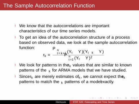
The Sample Autocorrelation Function

I We know that the autocorrelations are importantcharacteristics of our time series models.

I To get an idea of the autocorrelation structure of a processbased on observed data, we look at the sample autocorrelationfunction:

rk =

∑nt=k+1(Yt − Y )(Yt−k − Y )∑n

t=1(Yt − Y )2

I We look for patterns in the rk values that are similar to knownpatterns of the ρk for ARMA models that we have studied.

I Since rk are merely estimates of ρk , we cannot expect the rkpatterns to match the ρk patterns of a model exactly.

Hitchcock STAT 520: Forecasting and Time Series

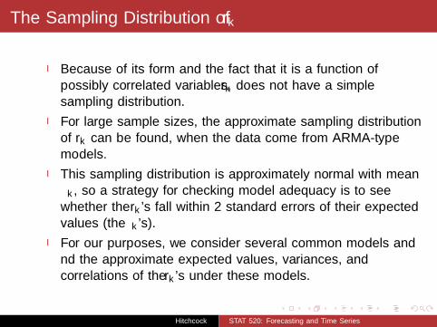
The Sampling Distribution of rk

I Because of its form and the fact that it is a function ofpossibly correlated variables, rk does not have a simplesampling distribution.

I For large sample sizes, the approximate sampling distributionof rk can be found, when the data come from ARMA-typemodels.

I This sampling distribution is approximately normal with meanρk , so a strategy for checking model adequacy is to seewhether the rk ’s fall within 2 standard errors of their expectedvalues (the ρk ’s).

I For our purposes, we consider several common models andfind the approximate expected values, variances, andcorrelations of the rk ’s under these models.

Hitchcock STAT 520: Forecasting and Time Series

The Sampling Distribution of rk Under Common Models

I First, under general conditions, for large n, rk is approximatelynormal with expected value ρk .

I If {Yt} is white noise, then for large n, var(rk) ≈ 1/n andcorr(rk , rj) ≈ 0 for k 6= j .

I If {Yt} is AR(1) having ρk = φk for k > 0, thenvar(r1) ≈ (1− φ2)/n.

I Note that r1 has smaller variance when φ is near 1 or −1.I And for large k :

var(rk) ≈ 1

n

[1 + φ2

1− φ2

]I This variance tends to be larger for large k than for small k ,

especially when φ is near 1 or −1.I So when φ is near 1 or −1, we can expect rk to be relatively

close to ρk = φk for small k , but not especially close toρk = φk for large k.

Hitchcock STAT 520: Forecasting and Time Series

The Sampling Distribution of rk Under the AR(1) Model

I In the AR(1) model,

corr(r1, r2) ≈ 2φ

√1− φ2

1 + 2φ2 − 3φ4

I For example, if φ = 0.9, then corr(r1, r2) = 0.97. Similarly, ifφ = −0.9, then corr(r1, r2) = −0.97.

I If φ = 0.2, then corr(r1, r2) = 0.38. Similarly, if φ = −0.2,then corr(r1, r2) = −0.38.

I Exhibit 6.1 on page 111 of the textbook gives other examplevalues for corr(r1, r2) and var(rk) for selected values of k andφ, assuming an AR(1) process.

I To determine whether a certain model (like AR(1) withφ = 0.9) is reasonable, we can examine the sampleautocorrelation function and compare the observed valuesfrom our data to those we would expect, under that model.

Hitchcock STAT 520: Forecasting and Time Series

The Sampling Distribution of rk Under the MA(1) Model

I For the MA(1) model, var(r1) = (1− 3ρ21 + 4ρ41)/n andvar(rk) = (1 + 2ρ21)/n for k > 1.

I Exhibit 6.2 on page 112 of the textbook gives other examplevalues for corr(r1, r2) and var(rk) for any k and selectedvalues of θ, under the MA(1) model.

I For the MA(q) model, var(rk) = (1 + 2∑q

j=1 ρ2j )/n for k > q.

Hitchcock STAT 520: Forecasting and Time Series

The Need to Go Beyond the Autocorrelation Function

I The sample autocorrelation function (ACF) is a useful tool tocheck whether the lag correlations that we see in a data setmatch what we would expect under a specific model.

I For example, in an MA(q) model, we know theautocorrelations should be zero for lags beyond q, so we couldcheck the sample ACF to see where the autocorrelations cutoff for an observed data set.

I But for an AR(p) model, the autocorrelations don’t cut off ata certain lag; they die off gradually toward zero.

Hitchcock STAT 520: Forecasting and Time Series

Partial Autocorrelation Functions

I The partial autocorrelation function (PACF) can be used todetermine the order p of an AR(p) model.

I The PACF at lag k is denoted φkk and is defined as thecorrelation between Yt and Yt−k after removing the effect ofthe variables in between: Yt−1, . . . ,Yt−k+1.

I If {Yt} is a normally distributed time series, the PACF can bedefined as the correlation coefficient of a conditional bivariatenormal distribution:

φkk = corr(Yt ,Yt−k |Yt−1, . . . ,Yt−k+1)

Hitchcock STAT 520: Forecasting and Time Series

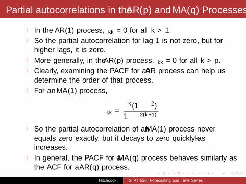
Partial autocorrelations in the AR(p) and MA(q) Processes

I In the AR(1) process, φkk = 0 for all k > 1.

I So the partial autocorrelation for lag 1 is not zero, but forhigher lags, it is zero.

I More generally, in the AR(p) process, φkk = 0 for all k > p.

I Clearly, examining the PACF for an AR process can help usdetermine the order of that process.

I For an MA(1) process,

φkk =θk(1− θ2)

1− θ2(k+1)

I So the partial autocorrelation of an MA(1) process neverequals zero exactly, but it decays to zero quickly as kincreases.

I In general, the PACF for a MA(q) process behaves similarly asthe ACF for a AR(q) process.

Hitchcock STAT 520: Forecasting and Time Series

Expressions for the Partial Autocorrelation Function

I For a stationary process with known autocorrelationsρ1, . . . , ρk , the φkk satisfy the Yule-Walker equations:

ρj = φk1ρj−1 + φk2ρj−2 + · · ·+ φkkρj−k , for j = 1, 2, . . . , k

I For a given k , these equations can be solved forφk1, φk2, . . . , φkk (though we only care about φkk).

I We can do this for all k .

I If the stationary process is actually AR(p), then φpp = φp,and the order p of the process is whatever is the highest lagwith a nonzero φkk .

Hitchcock STAT 520: Forecasting and Time Series

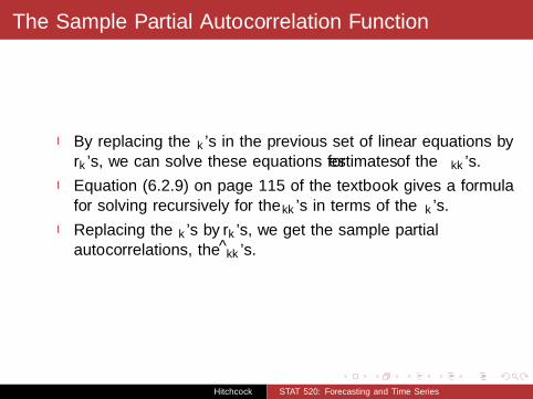
The Sample Partial Autocorrelation Function

I By replacing the ρk ’s in the previous set of linear equations byrk ’s, we can solve these equations for estimates of the φkk ’s.

I Equation (6.2.9) on page 115 of the textbook gives a formulafor solving recursively for the φkk ’s in terms of the ρk ’s.

I Replacing the ρk ’s by rk ’s, we get the sample partialautocorrelations, the φkk ’s.

Hitchcock STAT 520: Forecasting and Time Series

Using the Sample PACF to Assess the Order of an ARProcess

I If the model of AR(p) is correct, then the sample partialautocorrelations for lags greater than p are approximatelynormally distributed with means 0 and variances 1/n.

I So for any lag k > p, if the sample partial autocorrelation φkkis within 2 standard errors of zero (between −2/

√n and

2/√n), then this indicates that we do not have evidence

against the AR(p) model.

I If for some lag k > p, we have φkk < −2/√n or φkk > 2/

√n,

then we may need to change the order p in our model (orpossibly choose a model other than AR).

I This is a somewhat informal test, since it doesn’t account forthe multiple decisions being made across the set of values ofk > p.

Hitchcock STAT 520: Forecasting and Time Series

Summary of ACF and PACF to Identify AR(p) and MA(q)Processes

I The ACF and PACF are useful tools for identifying pureAR(p) and MA(q) processes.

I For an AR(p) model, the true ACF will decay toward zero.

I For an AR(p) model, the true PACF will cut off (becomezero) after lag p.

I For an MA(q) model, the true ACF will cut off (become zero)after lag q.

I For an MA(q) model, the true PACF will decay toward zero.

I If we propose either an AR(p) model or a MA(q) model foran observed time series, we could examine the sample ACF orPACF to see whether these are close to what the true ACF orPACF would look like for this proposed model.

Hitchcock STAT 520: Forecasting and Time Series

Extended Autocorrelation Function for Identifying ARMAModels

I For an ARMA(p, q) model, the true ACF and true PACF bothhave infinitely many nonzero values.

I Neither the true ACF nor the true PACF will cut off entirelyafter a certain number of lags.

I So it is hard to determine the correct orders of anARMA(p, q) model simply by using the ACF and PACF.

I The extended autocorrelation function (EACF) is one methodproposed to assess the orders of a ARMA(p, q) model.

I Other methods for specifying ARMA(p, q) models include thecorner method and the smallest canonical correlation (SCAN)method, which we will not discuss here.

Hitchcock STAT 520: Forecasting and Time Series

Some Details about the Extended AutocorrelationFunction Method

I In an ARMA(p, q) model, if we “filter out” (i.e., subtract off)the autoregressive component(s), we are left with a pureMA(q) process that can be specified using the ACF approach.

I For example, consider an ARMA(1, 1) model:

Yt = φYt−1 + et − θet−1.

I If we regress Yt on Yt−1, we get an inconsistent estimator ofφ, but this regression’s residuals do tell us about the behaviorof the error process {et}.

I So then let’s regress Yt on Yt−1 AND the lag 1 of the firstregression’s residuals, which stand in for et−1.

I In this second regression, the estimated coefficient of Yt−1

(call it φ) is a consistent estimator of φ.I Then Wt = Yt − φYt−1, having “filtered out” the

autoregressive part, should be approximately MA(1).

Hitchcock STAT 520: Forecasting and Time Series

More Details about the Extended Autocorrelation FunctionMethod

I For higher-order ARMA processes, we would need more ofthese sequential regressions to consistently estimate the ARcoefficients (we’d need q extra regressions for an AR(p, q)model).

I In practice, both AR order p and MA order q are unknown, sowe need to do this iteratively, considering grids of values for pand q.

I This iterative estimation of AR coefficients, assuming ahypothetical ARMA(k , j) model, produces “filtered” values

Wt,k,j = Yt − φYt−1 − · · · − φkYt−k

Hitchcock STAT 520: Forecasting and Time Series

Extended Sample Autocorrelations

I The extended sample autocorrelations are the sampleautocorrelations of Wt,k,j .

I If the hypothesized AR order k is actually the correct ARorder, p, and if the hypothesized MA order j ≥ q, then{Wt,k,j} is an MA(q) process.

I In that case, the true autocorrelations of Wt,k,j of lag q + 1 orhigher should be zero.

I We can try finding the extended sample autocorrelations for agrid of values of k = 0, 1, 2, . . . and a grid of values ofj = 0, 1, 2, . . ..

Hitchcock STAT 520: Forecasting and Time Series

The EACF in Table Form

I We can summarize the EACFs by creating a table with an“X” in the k-th row and j-th column if the lag j + 1 sampleautocorrelation of Wt,k,j is significantly different from zero.

I Since the sample autocorrelations are approximatelyN(0, 1/(n − k − j)) under the MA(j) process, the sampleautocorrelation is significantly different from zero if itsabsolute value exceeds 1.96/

√n − j − k .

I The table gets an “0” in its k-th row and j-th column if thelag j + 1 sample autocorrelation of Wt,k,j is NOT significantlydifferent from zero.

Hitchcock STAT 520: Forecasting and Time Series

The EACF in Table Form (Continued)

I The EACF table for an ARMA(p, q) process shouldtheoretically have a triangular pattern of zeroes with thetop-left zero occurring in the p-th row and q-th column (withthe row and column labels both starting from 0).

I (In reality, the sample EACF table will not be as clear-cut asthe examples that follow, since the sample EACF values havesampling variability.)

Hitchcock STAT 520: Forecasting and Time Series

Theoretical EACF Table for an ARMA(1, 1) Process

AR/MA 0 1 2 3 4 5 6 7 8 9 10

0 x x x x x x x x x x x1 x 0 0 0 0 0 0 0 0 0 02 x x 0 0 0 0 0 0 0 0 03 x x x 0 0 0 0 0 0 0 04 x x x x 0 0 0 0 0 0 05 x x x x x 0 0 0 0 0 06 x x x x x x 0 0 0 0 07 x x x x x x x 0 0 0 0

Hitchcock STAT 520: Forecasting and Time Series

Theoretical EACF Table for an ARMA(2, 3) Process

AR/MA 0 1 2 3 4 5 6 7 8 9 10

0 x x x x x x x x x x x1 x x x x x x x x x x x2 x x x 0 0 0 0 0 0 0 03 x x x x 0 0 0 0 0 0 04 x x x x x 0 0 0 0 0 05 x x x x x x 0 0 0 0 06 x x x x x x x 0 0 0 07 x x x x x x x x 0 0 0

Hitchcock STAT 520: Forecasting and Time Series