Chapter 6 Multiple Comparisons (Follow-up Tests) 6.1 A One-way Example The following is a textbook example taken from Neter et al.’s (1996) Applied linear statistical models [9]. The Kenton Food Company is interested in testing the effect of different package designs on sales. Five grocery stores were randomly assigned to each of four package designs. The package designs used either three or five colours, and either had cartoons or did not. Because of a fire in one of the stores, there were only four stores in the 5-colour cartoon condition. The dependent variable is sales, defined as number of cases sold. Actually, there are two independent variables: number of colours and presence versus absence of cartoons. But we will initially consider package design as a single categorical independent variable with four values. Sample Question 6.1.1 If there is a statistically significant relationship between package design and sales, would we be justified in concluding that differences in package design caused differences in sales? Answer to Sample Question 6.1.1 Yes, if the study is carried out prop- erly. It’s an experimental study. Sample Question 6.1.2 Is there a problem with external validity here? 138
Transcript
Chapter 6
Multiple Comparisons(Follow-up Tests)
6.1 A One-way Example
The following is a textbook example taken from Neter et al.’s (1996) Appliedlinear statistical models [9]. The Kenton Food Company is interested intesting the effect of different package designs on sales. Five grocery storeswere randomly assigned to each of four package designs. The package designsused either three or five colours, and either had cartoons or did not. Becauseof a fire in one of the stores, there were only four stores in the 5-colourcartoon condition.
The dependent variable is sales, defined as number of cases sold. Actually,there are two independent variables: number of colours and presence versusabsence of cartoons. But we will initially consider package design as a singlecategorical independent variable with four values.
Sample Question 6.1.1 If there is a statistically significant relationshipbetween package design and sales, would we be justified in concluding thatdifferences in package design caused differences in sales?
Answer to Sample Question 6.1.1 Yes, if the study is carried out prop-erly. It’s an experimental study.
Sample Question 6.1.2 Is there a problem with external validity here?
138
Answer to Sample Question 6.1.2 It’s impossible to tell for sure, butthere easily could be. The behaviour of the sales force would have to be con-trolled somehow. A double blind would be ideal.
The SAS program kenton.sas does a lot of things, starting with a one-way ANOVA using proc glm. The strategy will be to first present the entireprogram, and then go through it piece by piece and explain what is going on– with a few major digressions to explain the statistics.
reset noname; /* Makes output look nicer in this case */
print "Initial test has" numdf " and " dendf "degrees of freedom."
"Using significance level alpha = " alpha;
print s_table;
proc reg;
title2 ’Using proc reg and dummy variables’;
model sales = p1 p2 p3;
ncolour: test p1+p2 = p3; /* 3 vs 5 colours */
proc glm;
title2 "Actually it’s a two-way ANOVA";
class ncolours cartoon;
model sales = ncolours|cartoon;
/* The model statement could have been
model sales = ncolours cartoon ncolours*cartoon; */
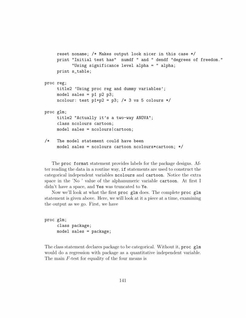
The proc format statement provides labels for the package designs. Af-ter reading the data in a routine way, if statements are used to construct thecategorical independent variables ncolours and cartoon. Notice the extraspace in the ’No ’ value of the alphanumeric variable cartoon. At first Ididn’t have a space, and Yes was truncated to Ye.
Now we’ll look at what the first proc glm does. The complete proc glm
statement is given above. Here, we will look at it a piece at a time, examiningthe output as we go. First, we have
proc glm;
class package;
model sales = package;
The class statement declares package to be categorical. Without it, proc glm
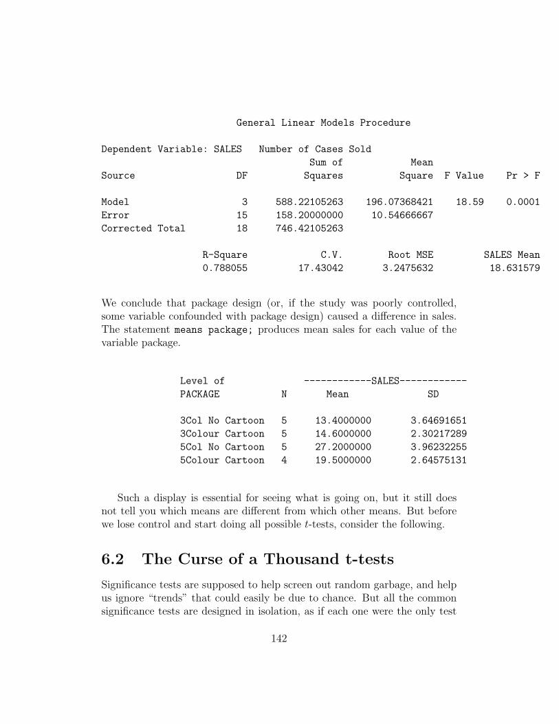
would do a regression with package as a quantitative independent variable.The main F -test for equality of the four means is
141
General Linear Models Procedure
Dependent Variable: SALES Number of Cases Sold
Sum of Mean
Source DF Squares Square F Value Pr > F
Model 3 588.22105263 196.07368421 18.59 0.0001
Error 15 158.20000000 10.54666667
Corrected Total 18 746.42105263
R-Square C.V. Root MSE SALES Mean
0.788055 17.43042 3.2475632 18.631579
We conclude that package design (or, if the study was poorly controlled,some variable confounded with package design) caused a difference in sales.The statement means package; produces mean sales for each value of thevariable package.
Level of ------------SALES------------
PACKAGE N Mean SD
3Col No Cartoon 5 13.4000000 3.64691651
3Colour Cartoon 5 14.6000000 2.30217289
5Col No Cartoon 5 27.2000000 3.96232255
5Colour Cartoon 4 19.5000000 2.64575131
Such a display is essential for seeing what is going on, but it still doesnot tell you which means are different from which other means. But beforewe lose control and start doing all possible t-tests, consider the following.
6.2 The Curse of a Thousand t-tests
Significance tests are supposed to help screen out random garbage, and helpus ignore “trends” that could easily be due to chance. But all the commonsignificance tests are designed in isolation, as if each one were the only test
142
you would ever be doing. The chance of getting significant results whennothing is going on may be about 0.05 (more or less, depending on how wellthe assumptions are met), but if you do a lot of tests on a data set thatis purely noise (no true relationships between any independent variable andany dependent variable), the chances of false significance mount up. It’s likelooking for your birthday in tables of stock market prices. If you look longenough, you will find it.
This problem definitely applies when you have a significant differenceamong more than two treatment means, and you want to know which ones aredifferent from each other. For example, in an experiment with 10 treatmentconditions (this is not an unusually large number, for real experiments), thereare 45 pairwise differences among means.
You have to pity the poor scientist who learns about this and is honestenough to take this problem seriously (let’s use the term “scientist” gener-ously to apply to anyone trying to use significance test to learn somethingabout a data set). On one hand, good scientific practice and common sensedictate that if you have gone to the trouble to collect data, you should ex-plore thoroughly and try to learn something from the data. But at the sametime, it appears that some stern statistical entity is scolding you, and sayingthat you’re naughty if you peek.
There are two main ways to resolve the dilemma. One is to basicallyignore the problem, while perhaps acknowledging that it is there. Accordingto this point of view, well, you’re crazy if you don’t explore the data. Maybethe true significance level for the entire process is greater than 0.05, but stillthe use of significance tests is a useful way to decide which results might bereal. Nothing’s perfect; let’s carry on.
The other reaction is to look for ways that significance tests can be mod-ified to allow for the fact that we’re doing a lot of them. What we want aremethods for holding the chances of false significance to a single low level fora set of tests, simultaneously. The general term for such methods is multi-ple comparison procedures. Often, when a significance test (like a one-wayANOVA) tests several things simultaneously and turns out to be significant,multiple comparison procedures are used as a second step, to investigatewhere the effect came from. In cases like this, the multiple comparisons arecalled follow-up tests, or post hoc tests, or sometimes probing.
It is generally acknowledged that multiple comparison methods are oftenhelpful (even necessary) for following up significant F -tests in order to seewhere an effect comes from. There is less agreement on how far the principle
143
should be extended. Personally, I like the idea of limiting the chance of falsesignificance to 0.05 for an entire study – say, for all the tests reported in ascientific paper, and all the ones that were not reported, too. This is a fairlyradical view, shared by almost no one. But it can work in practice if you haveenough data. More on this later. For now, let’s concentrate on following upa significant F test in a one-way analysis of variance.
In the Kenton package design data, there are 4 treatment conditions, and6 potential pairwise comparisons. The next line in the SAS program,
means package / bon tukey scheffe;
requests three kinds of multiple comparison tests for all pairwise differencesamong means.
6.2.1 Bonferroni
The Bonferroni method is very general, and extends far beyond pairwisecomparisons of means. It is a simple correction that can be applied whenyou are performing multiple tests, and you want to hold the chances of falsesignificance to a single low level for all the tests simultaneously. It applieswhen you are testing multiple sets of independent variables, multiple depen-dent variables, or both.
The Bonferroni correction consists of simply dividing the desired signifi-cance level (that’s α, the maximum probability of getting significant resultswhen actually nothing is happening, usually α = 0.05) by the number oftests. In a way, you’re splitting the alpha equally among the tests you do.
For example, if you want to perform 5 tests at joint significance level 0.05,just do everything as usual, but only declare the results significant at the joint0.05 level if one of the tests gives you p < 0.01 (0.01=0.05/5). If you want toperform 20 tests at joint significance level 0.05, do the individual tests andcalculate individual p-values as usual, but only believe the results of teststhat give p < 0.0025 (0.0025=0.05/20). Say something like “Protecting the20 tests at joint significance level 0.05 by means of a Bonferroni correction,the difference in reported liking between worms and spinach souffle was theonly significant food category effect.”
The Bonferroni correction is conservative. That is, if you perform 20tests, the probability of getting significance at least once just by chance isless than or equal to 0.0025 – almost always less. The big advantages of the
144
Bonferroni approach are simplicity and flexibility. It is the only way I knowto analyze quantitative and categorical dependent variables simultaneously.
The main disadvantages of the Bonferroni approach are
1. You have to know how many tests you want to perform in advance, andyou have to know what they are. In a typical data analysis situation,not all the significance tests are planned in advance. The results of onetest will give rise to ideas for other tests. If you do this and then applya Bonferroni correction to all the tests that you happened to do, it nolonger protects all the tests simultaneously. On the other hand, youcould randomly split your data into an exploratory sample and a repli-cation sample. Test to your heart’s content on the first sample. Then,when you think you know what your results are, perform only thosetests on the replication sample, and protect them simultaneously witha Bonferroni correction. This could be called ”Bonferroni-protectedcross-validation.” It sounds good, eh?
2. The Bonferroni correction can be too conservative, especially when thenumber of tests becomes large. For example, to simultaneously testall 780 correlations in a 40 by 40 correlation matrix at joint α = 0.05,you’d only believe correlations with p < 0.0000641 = 0.05/780.
Is this “too” conservative? Well, with n = 200 in that 40 by 40 example,you’d need r = 0.27 for significance (compared to r = .14 with nocorrection). With n = 100 you’d need r = .385, or about 14.8% of onevariable explained by another single variable. Is this too much to ask?You decide.
6.2.2 Tukey
This is Tukey’s Honestly Significant Difference (HSD) method. It is not hisLeast Significant Different (LSD) method, which has a better name but doesnot really get the job done. Tukey tests apply only to pairwise differencesamong means in ANOVA. It is based on a deep study of the probability dis-tribution of the difference between the largest sample mean and the smallestsample mean, assuming the population means are in fact all equal.
• If you are interested in all pairwise differences among means and noth-ing else, and if the sample sizes are equal, Tukey is the best (mostpowerful) test, period.
145
• If the sample sizes are unequal, the Tukey tests still get the job ofsimultaneous protection done, but they are a bit conservative. Whensample sizes are unequal, Bonferroni or Scheff can sometimes be morepowerful.
6.2.3 Scheffe
Suppose there are p treatments (groups, values of the categorical independentvariable, whatever you want to call them). A contrast is a special kindof linear combination of means in which the weights add up to zero. Apopulation contrast has the form
` = a1µ1 + a2µ2 + · · ·+ apµp
where a1 + a2 + · · · + ap = 0. The case where all of the a values are zerois uninteresting, and is excluded. A population contrast is estimated by asample contrast:
L = a1Y 1 + a2Y 2 + · · ·+ apY p.
By setting a1 = 1, a2 = −1, and the rest of the a values to zero we getL = Y 1 − Y 2, so it’s easy to see that any pairwise difference is a contrast.Also, the average of one set of means minus the average of another set is acontrast.
The initial F test for equality of p means can be viewed as a simultaneoustest of p− 1 contrasts. For example, suppose there are four treatments, andthe null hypothesis of the initial test is H0 : µ1 = µ2 = µ3 = µ4. The tablegives the a1, a2, a3, a4 values for three contrasts; if all three contrasts equalzero then the four population means are equal, and vice versa.
a1 a2 a3 a4
1 -1 0 00 1 -1 00 0 1 -1
The way you read this table is
µ1 - µ2 = 0µ2 - µ3 = 0
µ3 - µ4 = 0
146
Clearly, if µ1 = µ2 and µ2 = µ3 and µ3 = µ4, then µ1 = µ2 = µ3 = µ4,and if µ1 = µ2 = µ3 = µ4, then µ1 = µ2 and µ2 = µ3 and µ3 = µ4. Thesimultaneous F test for the three contrasts is 100% equivalent to a one-wayANOVA; it yields the same F statistic, the same degrees of freedom, and thesame p-value.
There is always more than one way to set up the contrasts to test agiven hypothesis. Staying with the example of testing differences amongfour means, we could have specified
a1 a2 a3 a4
1 0 0 -10 1 0 -10 0 1 -1
so that all the means are equal to the last one. These contrasts (differencesbetween means) are actually equal to the regression coefficients in a multipleregression with indicator dummy variables, in which the last category is thereference category. But no matter how you set up collection of contrasts, ifyou do it correctly you always get the same answer.
The Scheffe tests allow testing whether any contrast (or set of contrasts)of treatment means differs significantly from zero, with the tests for all possi-ble contrasts simultaneously protected at the same significance level, usually0.05.
When asked for Scheffe follow-ups to a one-way ANOVA, SAS tests allpairwise differences between means, but there are infinitely many more con-trasts in the same family that it does not do — and they are all jointlyprotected against false significance at the 0.05 level.
It’s a miracle. You can do infinitely many tests, all simultaneously pro-tected. You do not have to know what they are in advance. It’s an licensefor unlimited data fishing, at least within the class of contrasts of treatmentmeans. And you can test up to p − 1 contrasts simultaneously if you wish.They are all part of the same family.
Two more miracles:
• If the initial one-way ANOVA is not significant, it’s impossible for anyof the Scheffe follow-ups to be significant. This is not quite true ofBonferroni or Tukey.
• If the initial one-way ANOVA is significant, there must be a single con-trast that is significantly different from zero. It may not be a pairwise
147
difference, you may not think of it, and if you do find one it may notbe easy to interpret, but there is at least one out there. Well, actu-ally, there are infinitely many, but they may all be extremely similarto one another. Incidentally, if you test any collection of contrasts thatincludes a contrast that is significantly different from zero by a Scheffetest, then the Scheffe test for the collection will be significant too.
Given all this, clearly it is helpful to be able to test any set of contrast youwish. As you will see below, the contrast statement of proc glm lets youdo it easily. For now, let’s assume that you have done an initial F test fordifferences among p treatment means, it’s statistically significant, and alsoyou can get F tests for any contrast of collection of contrasts you specify.
As usual, the F tests for contrasts (which are sometimes optimisticallycalled “planned comparisons”) are designed in a vacuum, as if each one werethe only test you would ever do on your data. But you can convert them intoScheffe follow-ups to the initial test by using a different critical value (Recallthat if a test statistic is greater than the critical value, it’s significant).
Suppose that the follow-up test you want to do involves s contrasts; fora test of a single difference between means or some other single contrast,s = 1. Compute the usual F statistic for testing the contrast, and compareit to a modified critical value that we will call FS−crit; the S is for Scheffe.The formula for FS−crit is
FS−crit =p− 1
sFcrit, (6.1)
where Fcrit is the critical value for the initial test — the one you are followingup. You reject the null hypothesis and declare your Scheffe test significant ifF > FS−crit.
You can do as many of these tests as you want easily, using SAS and asmall table of FS−crit critical values. You can make the table you need withproc iml. This is illustrated in the example below; the code can easily bemodified to suit any problem. Or, you can use a textbook table of the Fdistribution and a calculator.
Please take another look at Formula (6.1). Notice that multiplying bythe number of means (minus one) is a kind of penalty for the richness ofthe infinite family of tests you could do, while dividing by the number ofcontrasts you’re testing reduces the penalty because you’re looking for some-thing bigger. As soon as Mr. Scheffe discovered these tests, people started
148
complaining that the penalty was very severe, and it was too hard to getsignificance. In my opinion, what’s remarkable is not that a license for un-limited fishing is expensive, but that it’s for sale at all. You can pay for itby increasing the sample size.
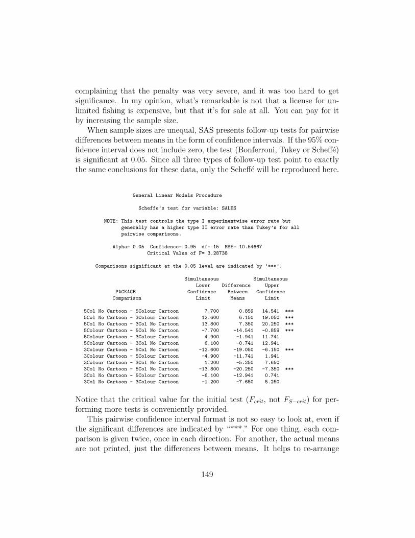
When sample sizes are unequal, SAS presents follow-up tests for pairwisedifferences between means in the form of confidence intervals. If the 95% con-fidence interval does not include zero, the test (Bonferroni, Tukey or Scheffe)is significant at 0.05. Since all three types of follow-up test point to exactlythe same conclusions for these data, only the Scheffe will be reproduced here.
General Linear Models Procedure
Scheffe’s test for variable: SALES
NOTE: This test controls the type I experimentwise error rate but
generally has a higher type II error rate than Tukey’s for all
pairwise comparisons.
Alpha= 0.05 Confidence= 0.95 df= 15 MSE= 10.54667
Critical Value of F= 3.28738
Comparisons significant at the 0.05 level are indicated by ’***’.
Simultaneous Simultaneous
Lower Difference Upper
PACKAGE Confidence Between Confidence
Comparison Limit Means Limit
5Col No Cartoon - 5Colour Cartoon 7.700 0.859 14.541 ***
5Col No Cartoon - 3Colour Cartoon 12.600 6.150 19.050 ***
5Col No Cartoon - 3Col No Cartoon 13.800 7.350 20.250 ***
5Colour Cartoon - 5Col No Cartoon -7.700 -14.541 -0.859 ***
3Colour Cartoon - 3Col No Cartoon 1.200 -5.250 7.650
3Col No Cartoon - 5Col No Cartoon -13.800 -20.250 -7.350 ***
3Col No Cartoon - 5Colour Cartoon -6.100 -12.941 0.741
3Col No Cartoon - 3Colour Cartoon -1.200 -7.650 5.250
Notice that the critical value for the initial test (Fcrit, not FS−crit) for per-forming more tests is conveniently provided.
This pairwise confidence interval format is not so easy to look at, even ifthe significant differences are indicated by “***.” For one thing, each com-parison is given twice, once in each direction. For another, the actual meansare not printed, just the differences between means. It helps to re-arrange
149
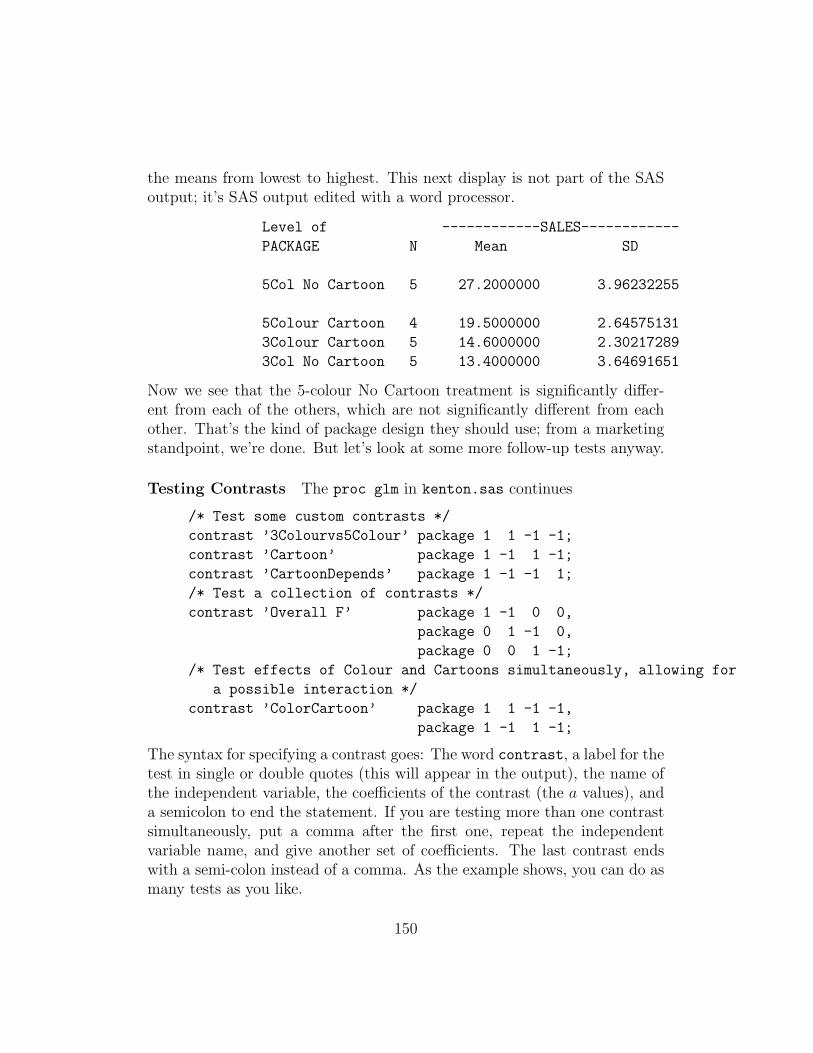
the means from lowest to highest. This next display is not part of the SASoutput; it’s SAS output edited with a word processor.
Level of ------------SALES------------
PACKAGE N Mean SD
5Col No Cartoon 5 27.2000000 3.96232255
5Colour Cartoon 4 19.5000000 2.64575131
3Colour Cartoon 5 14.6000000 2.30217289
3Col No Cartoon 5 13.4000000 3.64691651
Now we see that the 5-colour No Cartoon treatment is significantly differ-ent from each of the others, which are not significantly different from eachother. That’s the kind of package design they should use; from a marketingstandpoint, we’re done. But let’s look at some more follow-up tests anyway.
Testing Contrasts The proc glm in kenton.sas continues
/* Test some custom contrasts */
contrast ’3Colourvs5Colour’ package 1 1 -1 -1;
contrast ’Cartoon’ package 1 -1 1 -1;
contrast ’CartoonDepends’ package 1 -1 -1 1;
/* Test a collection of contrasts */
contrast ’Overall F’ package 1 -1 0 0,
package 0 1 -1 0,
package 0 0 1 -1;
/* Test effects of Colour and Cartoons simultaneously, allowing for
a possible interaction */
contrast ’ColorCartoon’ package 1 1 -1 -1,
package 1 -1 1 -1;
The syntax for specifying a contrast goes: The word contrast, a label for thetest in single or double quotes (this will appear in the output), the name ofthe independent variable, the coefficients of the contrast (the a values), anda semicolon to end the statement. If you are testing more than one contrastsimultaneously, put a comma after the first one, repeat the independentvariable name, and give another set of coefficients. The last contrast endswith a semi-colon instead of a comma. As the example shows, you can do asmany tests as you like.
150
6.2.4 Proper Follow-ups
We will describe a set of tests as proper follow-ups to to an initial test if
1. The null hypothesis of the initial test logically implies the null hypothe-ses of all the tests in the follow-up set.
2. All the tests are jointly protected against Type I error (false signifi-cance) at a known significance level, usually α = 0.05.
The first property requires explanation. First, consider that the Tukey tests,which are limited to pairwise differences between means, automatically sat-isfy this, because if all the population means are equal, then each pair isequal to each other. But it’s possible to make mistakes with Bonferroni andScheffe if you’re not careful.
Here’s why the first property is important. Suppose the null hypothesisof a follow-up test does follow logically from the null hypothesis of the initialtest. Then, if the null hypothesis of the follow-up is false (there’s reallysomething going on), then the null hypothesis of the initial test must beincorrect too, and this is one way in which the initial null hypothesis is false.Thus if we correctly reject the follow-up null hypothesis, we have uncoveredone of the ways in which the initial null hypothesis is false. In other words,we have (partly, perhaps) identified where the initial effect comes from.
On the other hand, if the null hypothesis of a potential follow-up testis not implied by the null hypothesis of the initial test, then the truth oruntruth of the follow-up null hypothesis does not tell us anything about thenull hypothesis of the initial test. They are in different domains. For example,suppose we conclude 2µ1 is different from 3µ2. Great, but if we want to knowhow the statement µ1 = µ2 = µ3 might be wrong, it’s irrelevant.
If you stick to testing contrasts as a follow-up to a one-way ANOVA,you’re fine. This is because if a set of population means are all equal, thenany contrast of those means is equal to zero. That is, the null hypothesisof the initial test automatically implies the null hypotheses of any potentialfollow-up test, and everything is okay. Furthermore, if you try to specify alinear combination that is not a contrast with the contrast statement ofproc glm, SAS will just say something like NOTE: CONTRAST SOandSO is
not estimable in the log file. There is no other error message or warning;the test just does not appear in your list file.
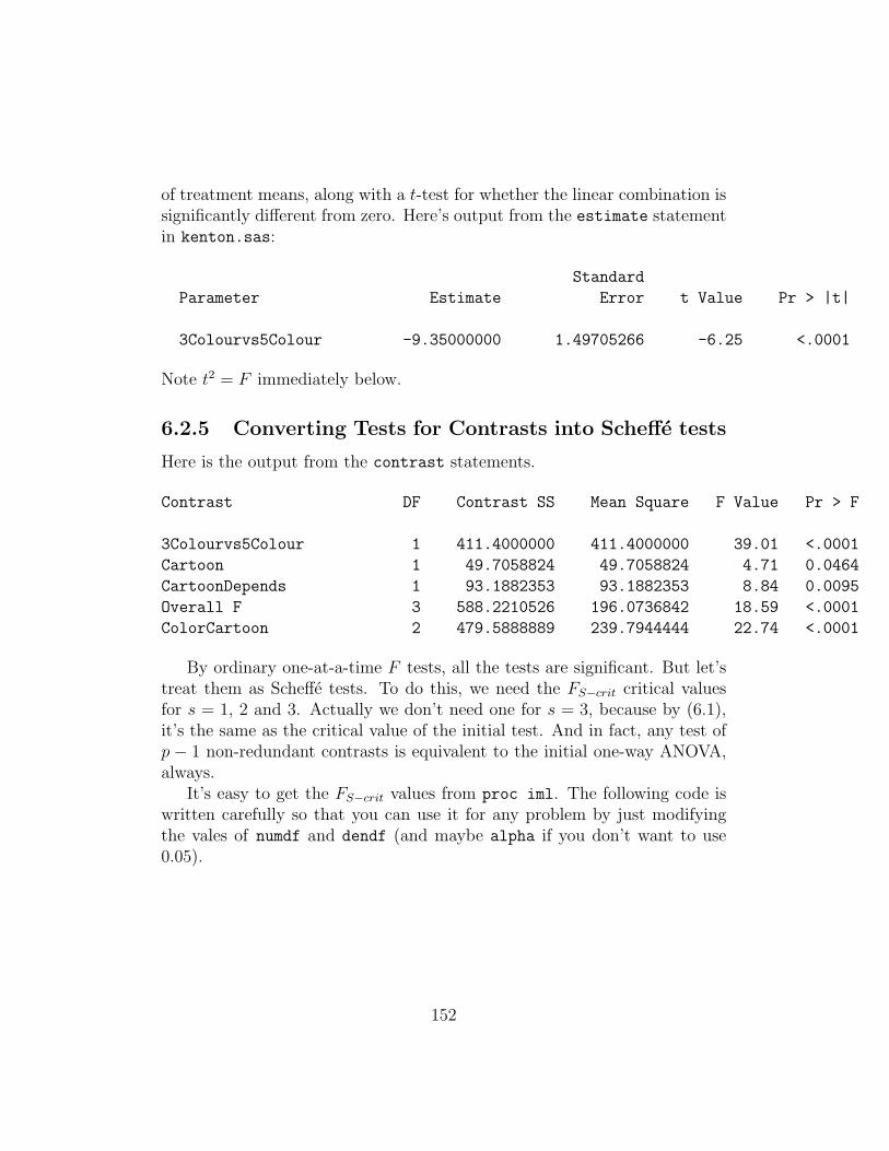
If you really want a linear combination that is not a contrast, use theestimate statement. It will give the sample value of any linear combination
151
of treatment means, along with a t-test for whether the linear combination issignificantly different from zero. Here’s output from the estimate statementin kenton.sas:
By ordinary one-at-a-time F tests, all the tests are significant. But let’streat them as Scheffe tests. To do this, we need the FS−crit critical valuesfor s = 1, 2 and 3. Actually we don’t need one for s = 3, because by (6.1),it’s the same as the critical value of the initial test. And in fact, any test ofp − 1 non-redundant contrasts is equivalent to the initial one-way ANOVA,always.
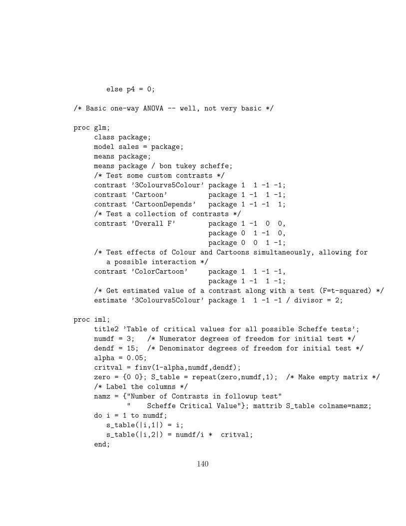
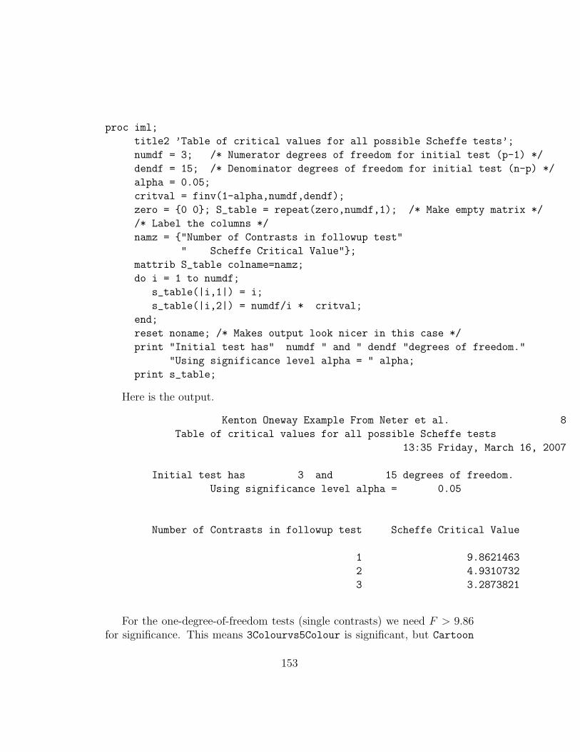
It’s easy to get the FS−crit values from proc iml. The following code iswritten carefully so that you can use it for any problem by just modifyingthe vales of numdf and dendf (and maybe alpha if you don’t want to use0.05).
152
proc iml;
title2 ’Table of critical values for all possible Scheffe tests’;
numdf = 3; /* Numerator degrees of freedom for initial test (p-1) */
dendf = 15; /* Denominator degrees of freedom for initial test (n-p) */
alpha = 0.05;
critval = finv(1-alpha,numdf,dendf);
zero = {0 0}; S_table = repeat(zero,numdf,1); /* Make empty matrix */
/* Label the columns */
namz = {"Number of Contrasts in followup test"
" Scheffe Critical Value"};
mattrib S_table colname=namz;
do i = 1 to numdf;
s_table(|i,1|) = i;
s_table(|i,2|) = numdf/i * critval;
end;
reset noname; /* Makes output look nicer in this case */
print "Initial test has" numdf " and " dendf "degrees of freedom."
"Using significance level alpha = " alpha;
print s_table;
Here is the output.
Kenton Oneway Example From Neter et al. 8
Table of critical values for all possible Scheffe tests
13:35 Friday, March 16, 2007
Initial test has 3 and 15 degrees of freedom.
Using significance level alpha = 0.05
Number of Contrasts in followup test Scheffe Critical Value
1 9.8621463
2 4.9310732
3 3.2873821
For the one-degree-of-freedom tests (single contrasts) we need F > 9.86for significance. This means 3Colourvs5Colour is significant, but Cartoon
153
and CartoonDepends are not, even though CartoonDepends has a p-value of0.0095 by the one-at-a-time test. ColourCartoon is also significant, because22.74 > 4.93. And of course Overall F is significant; it’s the initial test.
6.2.6 Extensions
This section provides a brief but very powerful extension of the Scheffe teststo multiple regression, and Scheffe-like tests for logistic regression.
Multiple Regression
Suppose the initial hypothesis is that d regression coefficients all are equalto zero. We will follow up the initial test by testing whether s linear combi-nations of these regression coefficients are different from zero; s ≤ d. Noticethat now we are testing linear combinations, not just contrasts. If a set ofcoefficients are all zero, then any linear combination (weighted sum) of thecoefficients is also zero. Thus the null hypotheses of the follow-up tests are im-plied by the null hypotheses of the initial test. As in the case of Scheffe testsfor contrasts in one-way ANOVA, using an adjusted critical value guaranteessimultaneous protection for all the follow-up tests at the same significancelevel as the initial test. This means we have proper follow-ups.
The formula for the modified critical value is
FS−crit =d
sFcrit, (6.2)
where again, the null hypothesis of the initial test is that d regression coef-ficients are all zero, and the null hypothesis of the follow-up test is that slinear combinations of those coefficients are equal to zero.
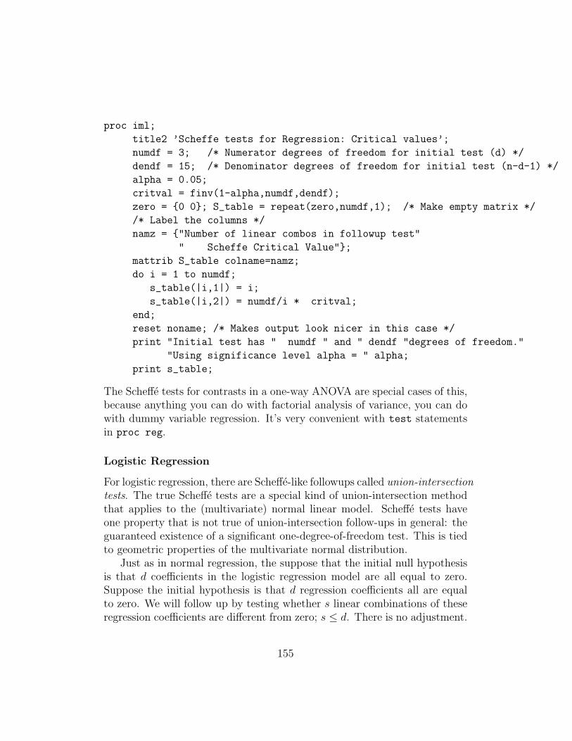
For convenience, here is the proc iml code to produce a table of adjustedcritical values.
154
proc iml;
title2 ’Scheffe tests for Regression: Critical values’;
numdf = 3; /* Numerator degrees of freedom for initial test (d) */
dendf = 15; /* Denominator degrees of freedom for initial test (n-d-1) */
alpha = 0.05;
critval = finv(1-alpha,numdf,dendf);
zero = {0 0}; S_table = repeat(zero,numdf,1); /* Make empty matrix */
/* Label the columns */
namz = {"Number of linear combos in followup test"
" Scheffe Critical Value"};
mattrib S_table colname=namz;
do i = 1 to numdf;
s_table(|i,1|) = i;
s_table(|i,2|) = numdf/i * critval;
end;
reset noname; /* Makes output look nicer in this case */
print "Initial test has " numdf " and " dendf "degrees of freedom."
"Using significance level alpha = " alpha;
print s_table;
The Scheffe tests for contrasts in a one-way ANOVA are special cases of this,because anything you can do with factorial analysis of variance, you can dowith dummy variable regression. It’s very convenient with test statementsin proc reg.
Logistic Regression
For logistic regression, there are Scheffe-like followups called union-intersectiontests. The true Scheffe tests are a special kind of union-intersection methodthat applies to the (multivariate) normal linear model. Scheffe tests haveone property that is not true of union-intersection follow-ups in general: theguaranteed existence of a significant one-degree-of-freedom test. This is tiedto geometric properties of the multivariate normal distribution.
Just as in normal regression, the suppose that the initial null hypothesisis that d coefficients in the logistic regression model are all equal to zero.Suppose the initial hypothesis is that d regression coefficients all are equalto zero. We will follow up by testing whether s linear combinations of theseregression coefficients are different from zero; s ≤ d. There is no adjustment.
155
The critical value for the follow-up tests is exactly that of the initialtest: a chi-square with d degrees of freedom. This principle appliesto both likelihood ratio and Wald tests. In fact, it is true of likelihood ratioand Wald tests in general, not just in logistic regression.
Bibliographic citation
If you want to report the use of union-intersection tests or Scheffe tests forregression, or even Scheffe tests for more than one contrast in a one-waydesign, you will have difficulty finding it in any published Statistics text.Like Scheffe’s original 1953 article [13], they almost universally stick to singlecontrasts. And it’s usually not too helpful to cite unpublished material likethis document.
Hochberg and Tamhane’s (1987) monograph Multiple comparison proce-dures [7] is a good source for the tests of multiple linear combinations inregression, of which the tests of contrasts presented here are a special case.It’s not very readable to non-statisticians, though. The same can be saidof Gabriel’s (1969) article [6], which is the primary source for the union-intersection follow-ups. But you can just trust me and cite them anyway.
156
Bibliography
[1] Bickel, P. J., Hammel, E. A., and O’Connell, J. W. (1975). Sexbias in graduate admissions: Data from Berkeley. Science, 187,398-403.
[2] Cody, R. P. and Smith, J. K. (1991). Applied statistics and theSAS programming language. (4th Edition) Upper Saddle River,New Jersey: Prentice-Hall.
[3] Cook, T. D. and Campbell, D. T. (1979). Quasi-experimentation:design and analysis issues for field settings. New York: RandMcNally.
[4] Feinberg, S. (1977) The analysis of cross-classified categoricaldata. Cambridge, Massachusetts: MIT Press.
[5] Fisher, R. A. (1925) Statistical methods for research workers. Lon-don: Oliver and Boyd.
[6] Gabriel, K. R. (1969). “Simultaneous test procedures — sometheory of multiple comparisons.” Ann. Math. Statist., 40, 224–250.
[7] Hochberg, Y., and Tamhane, A. C. (1987). Multiple comparisonprocedures. New York: Wiley.
[8] Moore, D. S. and McCabe, G. P. (1993). Introduction to the prac-tice of statistics. New York: W. H. Freeman.
[9] Neter, J., Kutner, M. H., Nachhtscheim, C. J. and Wasserman,W. (1996) Applied linear statistical models. (4th Edition) Toronto:Irwin.
157
[10] Roethlisberger, F. J. (1941). Management and morale. Cam-bridge, Mass.: Harvard University Press.
[11] Rosenthal, R. (1966). Experimenter effects in behavioral research.New York: Appleton-Century-Croft.
[12] Rosenthal, R. and Jacobson, L. (1968). Pygmalion in the class-room: teacher expectation and pupils’ intellectual development.New York: Holt, Rinehart and Winston.
[13] Scheffe, H. (1953). “A method for judging all contrasts in theanalysis of variance.” Biometrika, 40, 87–104.