Chapter 6

Probability and Random Processes

Random Experiment •  The fundamental concept in probability theory is the concept

of random experiment, which is any experiment whose outcome cannot be predicted with certainty

•  A simple example is coin tossing experiment. We know that heads and tails are possible outcomes, although the outcome (head or tail?) of a particular experiment (toss) is uncertain

Experiment Outcome

Random Experiment

A General Communication System •  k

Why Learn about Probability Theory? •  k

What is the probability that this is 1?

Back Probability Concepts

•  Example: Roll a dice

–  Outcomes: landing with a 1, 2, 3, 4, 5, or 6 face up. –  Sample Space: S ={1, 2, 3, 4, 5, 6} –  Event: outcome is larger than 4 –  Frequency of 1 happening = 10/60 = 1/6 (10 occurrence; 60 trials) –  We obtain Probability or Likelihood à We try INFINIT times!

Probability Concepts

Probability Axioms (P1-P3) •  ;

Probability Axioms •  [ Using P1-P3:

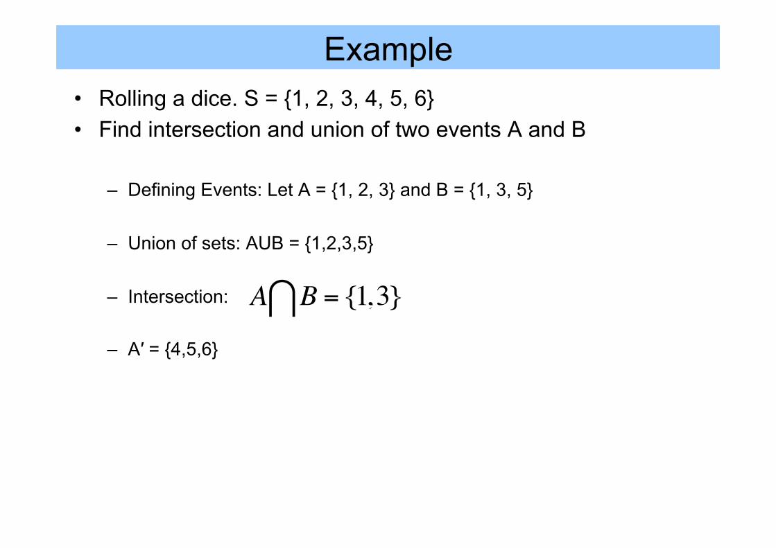
Example •  Rolling a dice. S = {1, 2, 3, 4, 5, 6} •  Find intersection and union of two events A and B

–  Defining Events: Let A = {1, 2, 3} and B = {1, 3, 5} –  Union of sets: AUB = {1,2,3,5}

–  Intersection: –  A′ = {4,5,6}

A B = {1,3}∩

Example of Union and Intersection •  A card is drawn from a well-shuffled deck of 52 playing

cards. What is the probability that it is a queen or a heart?

Conditional Probability •  l

a-pre-ori / a-poste-rio-rayh

Note: We are assuming A and B are not independent!

Independent Events •  k

Example •  1A & 1B •  1C

Rule  (Law)  of  Total  Probability

A

B1  

B2  B3  B4  

B5  

B6  B7  

( ) ( ) ( )∑= ii BAPBPAp |

Basically: we can calculate the probability of an event based on other events

Bayes’ Theorem (simple version) •  l

http://www.math.ucsd.edu/~gptesler/186/slides/bayesthm_14-handout.pdf

Full version of Bayes’ Theorem •  ,

http://www.math.ucsd.edu/~gptesler/186/slides/bayesthm_14-handout.pdf

Can you prove this?

Example •  1D •  1E

Example of Conditional Probability •  1

Given:

http://www.ece.tamu.edu/~georghiades/courses/ftp455/intro.pdf

Random Variable •  l

Discrete Random Variables •  ;

Continuous Random Variables •  A continuous random variable x takes values in a

continuous set of numbers. The range of x may include the whole real line or an interval thereof

•  Continuous random variables model many real life phenomena that include file download time on Internet, voltage across a resistor, and phase of a carrier signal produced by a radio transmitter

•  One characteristic that distinguishes a continuous random variable from the discrete one is that the probability of an individual outcome is zero. That is, , where x is any number in the range of x

•  Therefore, we can not use the PMF for a continuous random variable. Instead we shall use the cumulative distribution function which serves as an appropriate probability measure for any random variable

Example •  See notes DD1

Cumulative Distribution Function (CDF)

Z;x

Distribution Function

Density Function

Density Function

àPDF is a continuous random variable is a function which can be integrated to obtain the probability that the random variable takes a value in a given interval.

Example •  CC1- See notes

Common Discrete RVs •  Uniform •  Bernoulli •  Binomial •  Poisson

Uniform RV •  Totally Random – Equally likely events:

Bernoulli Random Variable •  Binary Random variable where 0 < p < 1 •  Bernoulli random variables are used to model random

experiments whose outcomes are binary –  For example, whether a bit is received in error, or whether a packet

is dropped by a congested router

Binomial Random Variable •  Binomial random variables model the number of successes

in a sequence of n independent trials of a random experiment, each of which yields success with probability p.

•  x RV is a binomial random variable if its PMF is of the form

Remember: Combination Example: Picking a team of 3 people from a group of 10. C(10,3) = 10!/(7! * 3!)

Poisson Random Variable •  ,

Examples •  AA1 •  BB1

Common Continuous Random Variables •  Here we introduce three important continuous random

variables: –  Uniform –  Gaussian –  Exponential –  Poisson –  Rayleigh

Uniform Random Variable •  ‘

Gaussian or Normal Random Variable •  LK

Gaussian or Normal Random Variable (contd) •  ;

Using Q-Function table Q(a) can be found!àNext

Standard Deviation

Gaussian or Normal Random Variable (properties)

•  Remember: –  Q-Function is the area under standard normal RV

•  Important Properties:

•  Integrals for Q(z cannot be evaluated in closed form.

However, for large values of z, very good closed-form approximations can be obtained, and for small values of z, numerical integration techniques can be applied easily. Approx.

Upp. Bound

Table of Q-Function

http://www.ece.ucdavis.edu/~levy/eec161/qfunc.pdf

Assuming SD = 1 and mean is 0

Example – Gaussian Distribution

Solution:

Example – Gaussian Distribution

Solution:

Use table to find the actual values

Mean = 12 - SD = sqrt (15)

Fχ (x) x=11 = Νm,σ (k)dk =1−−∞

x=11

∫ Q( x −mσ

)x=11

=1−Q( −130) =Q( 1

30)

Exponential Random Variable •  ;’

Summary

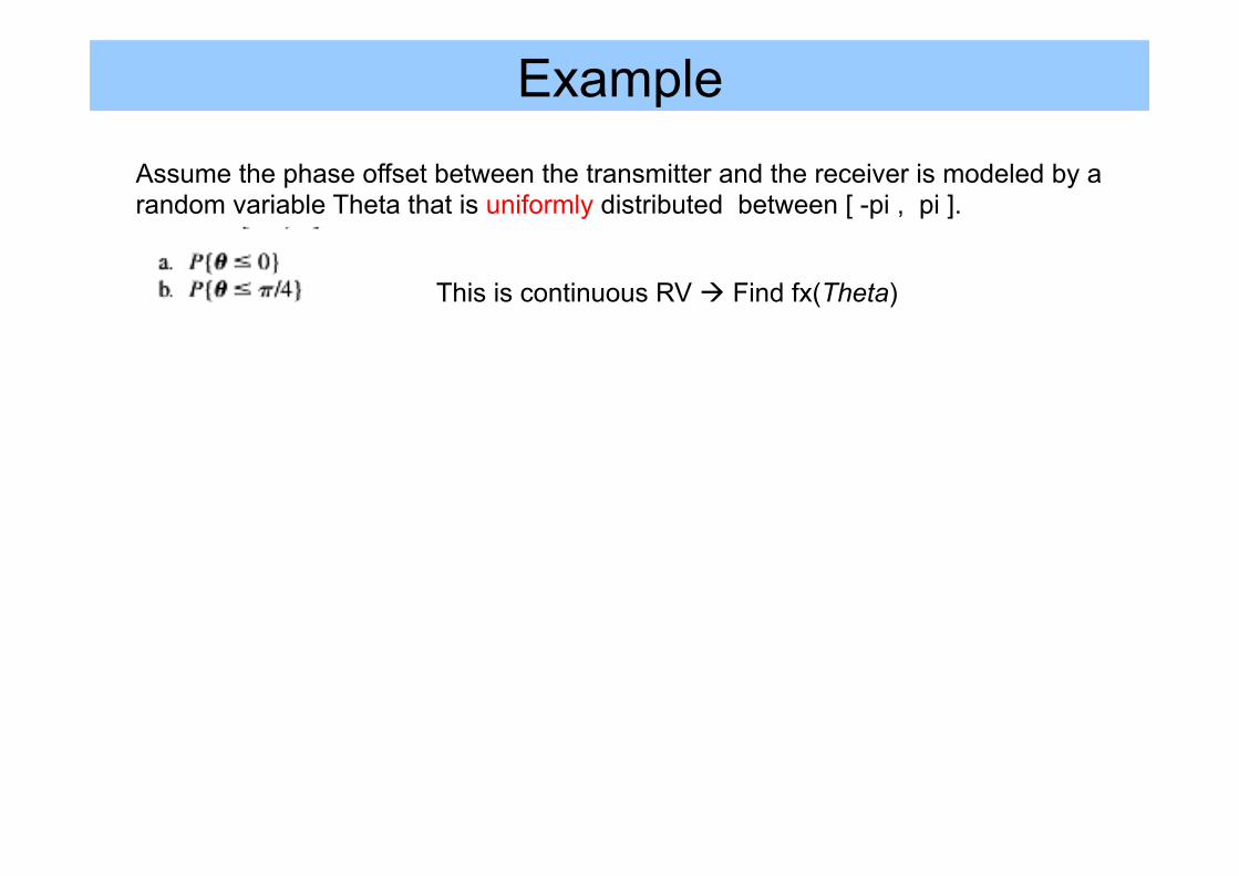
Example Assume the phase offset between the transmitter and the receiver is modeled by a random variable Theta that is uniformly distributed between [ -pi , pi ].

This is continuous RV à Find fx(Theta)

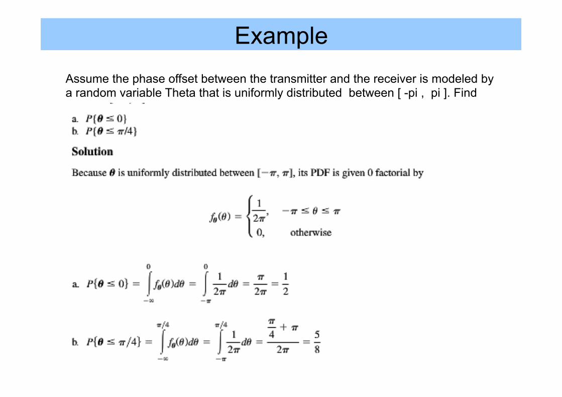
Example Assume the phase offset between the transmitter and the receiver is modeled by a random variable Theta that is uniformly distributed between [ -pi , pi ]. Find

Poisson Random Variable •  ,

Statistics of RV •  Finding behaviors using certain averages

–  Mean, Variance, Standard Deviation, Moments, Central Moments, etc.

Describes the spread of its PDF around the expected value

Statistics of RV (cont.) •  Variance •  Root-Mean-Square

•  Note that when mean is zero variance is the same as RMS:

•  Standard Deviation of a RV is

Moments of a RV •  Expected value E{x} is the First Moment of a RV •  RMS value E{x^2} is the Second Moment of a RV •  The nth moment of a real-valued random variable x is

•  The nth central moment of a real-valued random variable x is

•  Hence the variance Var ( x ) is the second central moment of x

Example 1 – Mean & Variance •  x

Example 1 – Mean & Variance •  X

•  The nth moment (integ. by part):

•  Thus, for n=0àE{x^0}=1 (*)

Integration Table (number 57 – Ingration by part) http://www.sonoma.edu/users/f/farahman/sonoma/courses/es430/resources/integral-table.pdf

Zero

(*)

= Second moment – first moment square!

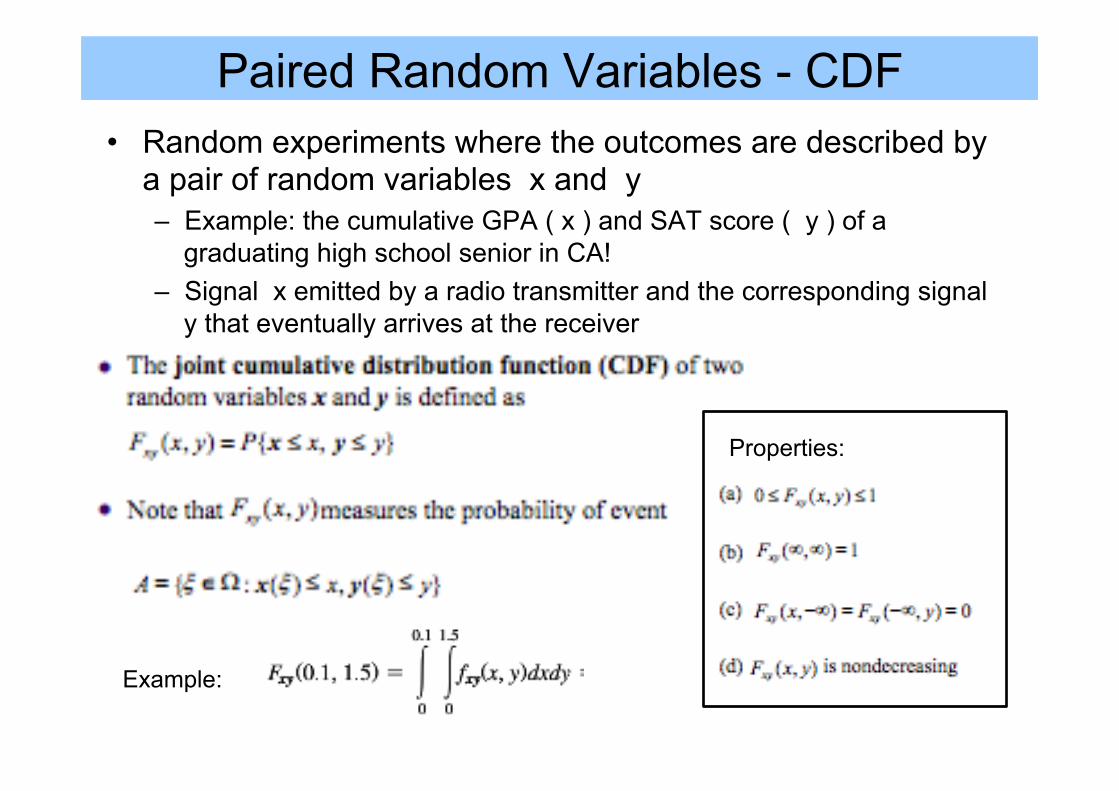
Paired Random Variables - CDF •  Random experiments where the outcomes are described by

a pair of random variables x and y –  Example: the cumulative GPA ( x ) and SAT score ( y ) of a

graduating high school senior in CA! –  Signal x emitted by a radio transmitter and the corresponding signal

y that eventually arrives at the receiver

• 

Properties:

Example:

Paired Random Variables - PDF •  k

Properties:

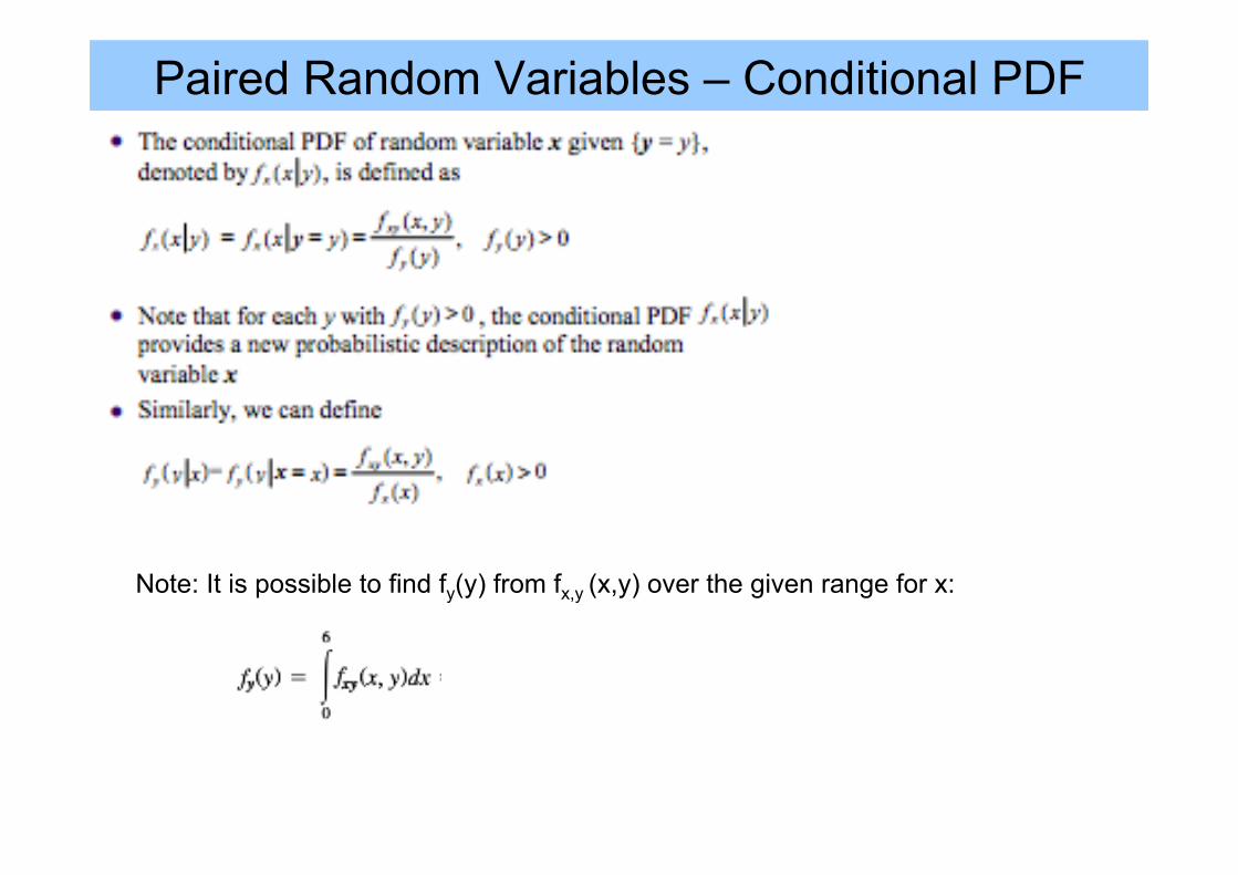
Paired Random Variables – Conditional PDF •  l

Note: It is possible to find fy(y) from fx,y (x,y) over the given range for x:

Statistically Independent RV •  l

Statistics of Paired RV •  k

Correlation and Covariance of Two RVs •  kk

Corr. Corf is between 0 & 1 If CC = 0 à two RVs are uncorrelated If CC >= 0 à two RVs are moving in the same direction If CC < 0 à two RVs are moving in different directions

i.i.d RVs and Central Limit Theorem Let x1, x2, …. be n independent, identically distributed random variables with finite mean and variance We consider their scaled sumà •  The CDF of zn converges to a Gaussian CDF as n

approaches ∞, independent of the distribution of random variables xn

•  In a nutshell, the central limit theorem, states that the sum of almost any set of independent and randomly generated random variables rapidly converges to the Gaussian distribution λ

•  This explains why the Gaussian distribution arises so commonly in practice to reflect the additive effect of multiple random occurrences

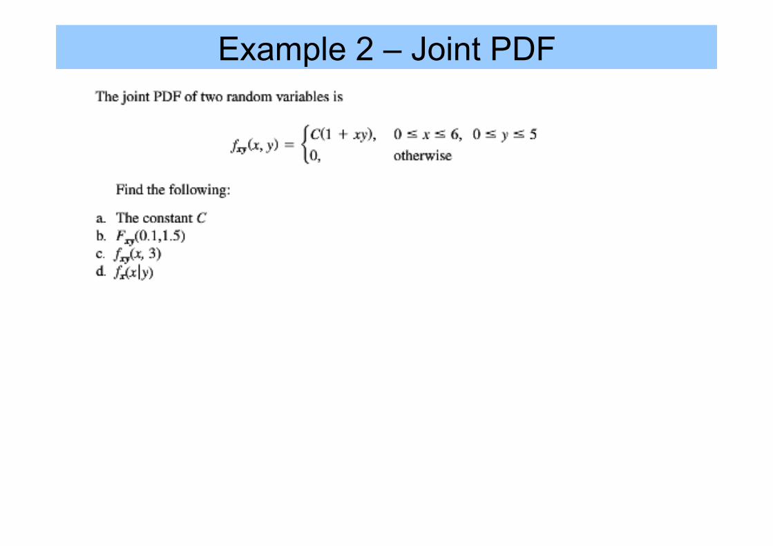
Example 2 – Joint PDF •  o

Example 3 – Statistical Averages

Outline •  Later

References •  Leon W. Couch II, Digital and Analog Communication

Systems, 8th edition, Pearson / Prentice, Chapter 6 •  "M. F. Mesiya, ”Contemporary Communication Systems”,

1st ed./2012, 978-0-07-. 338036-0, McGraw Hill. Chapter 6