Chapter 6: Synchronisation Synchronisation occurs when large numbers of individuals co-ordinate to act in unison. In this wide definition of the word, many different types of collective behaviour are examples of synchronisation. A highly aligned group of birds, fish or particles can be said to have synchronised their direction of movement. More commonly however, when we use the word synchronisation we are thinking about time. Bank robbers synchronise their watches before a robbery, the instruments of the orchestra are synchronised by the conductor and the sound is synchronised to the pictures in a film. It is this narrower sense of the word synchronisation I use in this chapter. How and why do behaviours become synchronised in time?

Given that synchronisation is a specific type of collective behaviour it should come as no surprise that it shares many properties with systems looked at in earlier chapters of this book. In particular, and unlike with the bank robbers or the orchestra, synchronisation can be achieved without a leader or centralised control. As with other types of collective behaviour, we can also build mathematical models that describe how synchronisation emerges from individual interactions. Indeed, some of the models of synchronisation are among the most elegant models of collective behaviour and have been employed successfully in understanding a wide variety of biological and social systems.

6.1 Rhythmic synchronisation While the instruments of a concert orchestra are, at least in part, synchronised by signals from the conductor, the applause of the audience after the performance is not usually centrally controlled. Despite the lack of a central controller, in Eastern Europe and Scandinavia this applause is often rhythmical, with the entire audience clapping simultaneously and periodically. Neda et al. (2000a; 2000b) recorded and analysed the clapping of theatre and opera audiences in Romania and Hungary and found a common pattern: first an initial phase of incoherent but loud clapping, followed by a relatively sudden jump into synchronised clapping that, after about half a minute, was again rapidly replaced by unsynchronised applause (figure 6.1a). A surprising observation was that the average volume of the synchronised clapping is lower than that of unsynchronised applause, both before and after the synchronised bouts. While an audience presumably wants to maximise their volume and thus their appreciation of the performance, they are unable to combine louder volumes with synchronised clapping.

Neda and co-workers went on to record small local groups in the audience and asked individuals, isolated in a room, to clap as if (I) “at the end of a good performance” or (II) “during rhythmic applause”. Both modes of clapping were rhythmical at the individual level, with individuals clapping in mode I twice as fast as those clapping in mode II (figure 6.1b). The important difference was in the

between individual variation for the two modes. When asked to clap rhythmically, isolated individuals chose similar, though not precisely identical, clapping frequencies, while when given the freedom to applaud spontaneously the chosen frequencies spread over a much wider range.

To interpret this observation, Neda et al. (2000b) used a classical mathematical result about coupled oscillators. Kuramoto (1975) studied a model of a large number of oscillators, each with its own frequency but coupled together so that they continually adjust their frequency to be nearer that of the average frequency. Kuramoto showed that provided the oscillators’ initial frequencies are not too different they will eventually adopt the same frequency and

Figure 6.1: The emergence of synchronised clapping (reproduced from Neda et al. 2000a). (a) The average noise intensity of a crowd through time. The first 10 seconds shows unsynchronised fast clapping, followed by a change to regular slower clapping until around 27 seconds, followed by synchronised clapping again. (b) A normailised histogram of clapping frequencies for 73 high school students (isolated from each other) for Mode I (solid lines) and Mode II (dotted lines) clapping.

oscillate synchronously (Kuramoto 1984). This is what happens to audiences clapping according to mode II. Their initial independent clapping frequencies are close together, and by listening to the clapping of others, they synchronise their clapping. Audiences clapping in mode I have initial frequencies which are less similar to each other. Thus even if they try to adjust their clapping in reaction

(a)

(b)

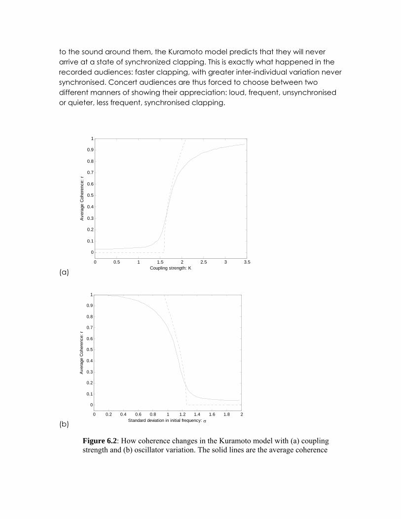
to the sound around them, the Kuramoto model predicts that they will never arrive at a state of synchronized clapping. This is exactly what happened in the recorded audiences: faster clapping, with greater inter-individual variation never synchronised. Concert audiences are thus forced to choose between two different manners of showing their appreciation: loud, frequent, unsynchronised or quieter, less frequent, synchronised clapping.

(a)0 0.5 1 1.5 2 2.5 3 3.5

0

0.1

0.2

0.3

0.4

0.5

0.6

0.7

0.8

0.9

1

Coupling strength: K

Ave

rage

Coh

eren

ce: r

(b)0 0.2 0.4 0.6 0.8 1 1.2 1.4 1.6 1.8 2

0

0.1

0.2

0.3

0.4

0.5

0.6

0.7

0.8

0.9

1

Standard deviation in initial frequency: σ

Ave

rage

Coh

eren

ce: r

Figure 6.2: How coherence changes in the Kuramoto model with (a) coupling strength and (b) oscillator variation. The solid lines are the average coherence

after 2000 time steps over 1000 runs of N=800 oscillators. The dotted line in (a) is the approximation

⎟⎟⎠

⎞⎜⎜⎝

⎛ −≈

C

C

KKKr π where σ

π

32=CK . In this simulation σ=1 (b) The dotted line

is the approximation ⎟⎠⎞

⎜⎝⎛ −

≈σσσπ Cr where KC 32

πσ = . In this simulation

K=2.

Box 6.A: The Kuramoto model. Kuramoto (1975; 1984) proposed a simple model for the synchronisation of coupled oscillators. Kuramoto assumed that the frequency, i.e. the rate of change, of the phase, θi, of each oscillator, k, was determined by

∑=

−+=N

jkjk

k

NK

dtd

1

)sin( θθωθ (equation 6.A.1)

where N is the number of oscillators and K is the strength of coupling between the oscillators. ωk

is the natural frequency of the oscillator, the frequency it will adopt if it is not coupled to other oscillators (i.e. when K=0). Under this model, each oscillator adjusts its frequency in response to the phases of the other oscillators. If oscillator k has a smaller phase than the average phase of all other oscillators then it will increase its frequency and thus become more in phase with the other oscillators. Likewise, if oscillator k has a larger phase than average then it will decrease its frequency.

Intuitively, we would expect such a regulation to result in the phases of the oscillators becoming more similar. What is less clear is how we expect the degree of synchronisation to change as a function of the coupling strength, or of the initial frequency differences between the oscillators. Kuramoto defined the coherence, i.e. the degree of phase synchronisation, between the oscillators to be the complex number

∑=

=N

j

ii jeN

re1

1 θψ (equation 6.A.2)

where 1−=i . By recalling the definition of a complex number, , and doing some algebraic manipulation we see that

))sin()(cos( ψψψ irrei +=

∑=

=N

jjN 1

1 θψ and

2

1

2

1sincos1

⎟⎟⎠

⎞⎜⎜⎝

⎛+⎟⎟

⎠

⎞⎜⎜⎝

⎛= ∑∑

==

N

jj

N

jjN

r θθ

Thus ψ gives the average frequency and r is a measure of the variation between the frequencies of the oscillators. When all the oscillators have the same phase, ψθ =j , then

1sincos1 2222 =+= ψψ NNN

r . If all oscillators have a random phase, independent of

that of the other oscillators, then as N→∞, r→0. Thus larger values of r indicate a more coherent population of oscillators.

Figure 6.2 shows how coherence changes with the variation of the initial frequency, i.e. the standard deviation of the distribution of the ωk. When the standard deviation is small r is large. As the standard deviation increases r decreases. There is a critical level of between-oscillator variation, above which there is no coherence and below which coherence begins to emerge.

The definitions of r and ψ not only provide a convenient way of measuring coherence, but also allow an elegant mathematical analysis of Kuramoto’s original model. A more detailed mathematical discussion of Kuramoto’s model is provided in Strogatz (2000) . Here I summarise some of the main results presented by Strogatz. If we multiply both sides of equation 6.A.2 by

and then equate the complex parts we get kie θ−

∑=

−=−N

jkjk N

r1

)sin(1)sin( θθθψ

Substituting this into equation 6.A.1 we see that

)sin( kkk rK

dtd θψωθ

−+= equation 6.A.3

When the coherence r is small or the coupling K is weak then the pull away from the natural frequency is small. Conversely, strongly coupled oscillators with high coherence have a strong pull away from the natural frequency.

Kuramoto assumed an infinite number of oscillators with initial frequencies kω taken from a

distribution with a symmetrical probability density function with mean ψ=0, e.g. the Normal distribution. From equation 6.A.3 we see that at equilibrium

)sin( kk rK θω =

Those oscillators with rKk <ω approach this equilibrium, while those with rKk >ω ‘drift’

without arriving at the equilibrium. Kuramoto went on to derive a number of useful results. For example, if the kω are initially normally distributed with mean 0 and variance σ2 then

synchronisation occurs, i.e. r>0, whenever σπ

32>K . Below the critical value σ

π

32=CK

the oscillators all act independently of each other. For values of K slightly above this critical value the proportion of the synchronised oscillators is

⎟⎟⎠

⎞⎜⎜⎝

⎛ −≈

C

C

KKKr π

Figure 6.2a compares this approximation with an average outcome of 1000 simulations of 800 oscillators.

The importance of Kuramoto’s model, which is presented in detail in Box 6.A, is that it shows that individuals with slightly different frequencies can synchronise, each by moving their frequency slightly towards the average. It further predicts that above some critical level of between-individual variation synchronisation does not occur at all (figure 6.2). In their empirical study, Neda et al. proposed that the opera crowds with unsynchronised clapping have a level of intrinsic variation above this critical level and those with synchronised clapping to have an intrinsic variation below the critical level. The switch in clapping mode from I to II reduces the between-individual variation and synchronisation ensues.

Synchronised rhythmic activity is seen in many different animal groups and across much of biology (Strogatz 2003). As discussed in chapter 1, the oestrus cycles of female lions are usually synchronised within a pride (Bertram 1975) and the phase of these oscillations can be reset by the takeover of the pride by a new male (Packer & Pusey 1983). Likewise, human females’ menstrual cycles become synchronised when the females are living or working closely together (Stern & McClintock 1998). For many systems there is a good understanding of the physiological mechanisms involved in coupling individuals. Probably the best understood mechanism within animal behavior is the simultaneous flashing of some species of fireflies (Buck 1988; Buck & Buck 1976). Isolated fireflies flash approximately once every second, but if they are subjected to an artificial flash at some point between flashes then their next flash is suppressed until approximately 1 second after the artificial flash (Buck et al. 1981). Mirollo & Strogatz (1990) developed a model to show that such phase resetting oscillators will synchronise, although they deal only with the case where all oscillators have the same intrinsic frequency. A number of good reviews have been written both of firefly flashing (Buck & Buck 1976; Camazine et al. 2001) and rhythmic synchronisation in general (Strogatz 2003; Strogatz & Stewart 1993).

6.2 Stochastic synchronisation Anyone who has seen a flock of sheep or a group of hens pecking in a farmyard knows that domestically farmed animals commonly synchronise their behaviour. Hens (Hughes 1971), pigs (Nielsen B et al. 1996) and sheep (Rook A & Penning P 1991) are just some examples of animals that feed simultaneously. While simultaneous feeding may in part be accounted for by synchronised circadian rhythms and environmental cues, it can also be due to increased feeding in response to the feeding of others. For example, Barber (2001) found that laying hens were more motivated to feed in the presence of feeding companions.

Collins & Sumpter (2007) looked at how the number of feeding chickens at a particular point in a commercial chicken house influenced the rate at which other chickens began feeding nearby. Chicken houses are large homogeneous

0 1 2 3 4 5 6 70

0.2

0.4

Number at feeder

Freq

uenc

y(d)

0 1 2 3 4 5 6 70

0.2

0.4

Number at feeder

Freq

uenc

y

0

1

2

3

4

5

Tim

e (m

inut

es)

Position along the feeder5 10 15

2000

2050

2100

2150

2200

0

1

2

3

4

5

Tim

e (m

inut

es)

Position along the feeder0 5 10 15

0

2

4

6

8

(b)(a)

(c)

Figure 6.3: Comparison of simulation model and observations of real chickens. (a) Example of simulated number of birds feeding at different sections along the feeder through 200 simulated minutes (b) The distribution of number of chickens feeding per three adjacent feeding sections over 10,000 simulated minutes (c) Example of activity at different sections along a real chicken feeder through 10 minutes and (d) distribution of number of chickens feeding per three adjacent feeding sections over these 10 minutes. Fitted lines in (b) and (d) show distribution of number of chickens assuming a Poisson distribution. See Collins & Sumpter (2007) for parameter values and details of the model and experimental setup.

environments where a supply of food is provided along a feeding trough. The food constantly moves along this trough, ensuring that the supply is equal at all points of the feeder and that, in the absence of other birds, no part of the environment is consistently more attractive to the birds than any other. Figure 3.7 shows how the rate at which chickens join and leave a point at a feeding trough changed as a function of the number of birds already at that point. As the number of chickens feeding at a point increases, the rate of arrival increases and the rate of leaving decreases.

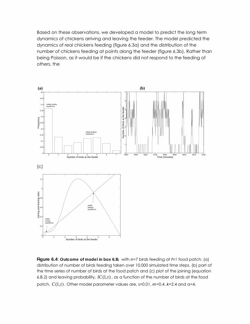
Based on these observations, we developed a model to predict the long term dynamics of chickens arriving and leaving the feeder. The model predicted the dynamics of real chickens feeding (figure 6.3a) and the distribution of the number of chickens feeding at points along the feeder (figure 6.3b). Rather than being Poisson, as it would be if the chickens did not respond to the feeding of others, the

(a) (b)

0 1 2 3 4 5 6 70

0.05

0.1

0.15

0.2

0.25

0.3

0.35

0.4

0.45

0.5

Number of birds at the feeder

Fre

quen

cy

stable restingequilibrium

stable feedingequilibrium

8400 8500 8600 8700 8800 8900 9000 9100 92000

1

2

3

4

5

6

7

Time (minutes)

Num

ber

of b

irds

at th

e fe

eder

(c)

0 1 2 3 4 5 6 70

0.2

0.4

0.6

0.8

1

1.2

Number of birds at the feeder

Join

ing

and

leav

ing

rate

s

stablerestingequilibrium

stablefeedingequilibrium

Figure 6.4: Outcome of model in box 6.B. with n=7 birds feeding at f=1 food patch. (a) distribution of number of birds feeding taken over 10,000 simulated time steps. (b) part of the time series of number of birds at the food patch and (c) plot of the joining (equation 6.B.2) and leaving probability, , as a function of the number of birds at the food

patch, . Other model parameter values are, s=0.01, m=0.4, k=2.4 and α=4. ),1( tlC

),1( tC

distribution is skewed towards observations of either none or lots of chickens at the feeder. A qualitatively similar distribution was seen in further observations of the number of chickens at the feeder through space and time (figure 6.3c,d). The sharp quorum response and positive feedback mean that, despite no environmental differences along different sections of the feeder, at any one time certain parts of the feeder will be preferred over others.

Box 6.B: Stochastic Synchronisation of feeding.

Box 3.C in chapter 3 describes a model of birds which choose to feed at particular food patch as an increasing function of the number of birds already at that patch. Here, we consider a simulation of this model with access to only one food patch, f=1. Birds can either forage at the food patch or rest away from the food patch. The probability of per bird not at the food patch of joining a food patch is

⎟⎟⎠

⎞⎜⎜⎝

⎛+

−+ αα

α

),1(),1()(

tCktCsms (6.B.1)

and the probability per bird leaving the food patch is a constant (see Box 3.C for an explanation of the parameters).

Figure 6.3MODELb shows a time series of how many birds are visiting the feeder for a simulation of a group of n=7 birds. Figure 6.3a shows the distribution through time of individuals at the food patch. There are frequently periods where there are no birds at the food patch and periods where nearly all the birds at the food. These resting and feeding periods are relatively stable with most of the birds synchronizing their feeding bouts.

To help understand how this synchronization arises, figure 6.3c shows the average number of birds joining the food patch per time step, i.e.

( ) ⎟⎟⎠

⎞⎜⎜⎝

⎛+

−+− αα

α

),1(),1()(),1(

tCktCsmstCn (6.B.2)

as a function of the number of birds on the patch. The probability of one bird going to the feeder when there are none there is relatively small, but once one bird is there, there is a greater probability that another bird arrives than that the bird leaves. Furthermore, once two birds are there the probability of arriving becomes greater still until the number of birds climbs up to between 3 or 4. The average number of birds leaving the food patch per time step is and is also shown in figure 6.3c.

),1( tlC

The points at which the average joining and leaving rates are equal correspond to feeding equilibriums. There are three such equilibrium, the smallest of which corresponds to a stable resting equilibrium and the largest of corresponding to a stable feeding equilibrium. The middle equilibrium is unstable, such that if by chance the number of feeding birds drops below this unstable equilibrium then the birds quickly equilibriate at mostly resting. Alternatively, if the number of feeding birds go above the unstable equilibrium, the number of feeding birds quickly equilibriates with three or four feeding. Thus the number of birds at the food patch jumps between the two stable equilibrium of none and, alternatively, three to four birds at the patch.

Box 6.B presents a simplified version of the chicken feeding model for a group of seven chickens visiting only a single feeder. Figure 6.4 illustrates how synchronised feeding occurs in this model. The birds alternate between most of them feeding and nearly all resting, but are not periodic in their feeding bouts. During resting periods there are small fluctuations with some individuals engaging in feeding. At some point these fluctuations take the number of individuals to a level at which the average rate of joining the feeder exceeds the average rate of leaving. Now the population quickly climbs where the majority of birds are feeding. Further fluctuations around this equilibrium eventually lead to the number of foragers falling again to close to zero. This pattern continues, but with no clearly defined frequency.

Gautrais et al. (2007) found that small groups of sheep synchronise their bouts of activity, and these bouts are not necessarily periodic. They fitted a Markov chain model to the data, where the state of the model was the number of active individuals. The measured transition probabilities of the Markov chain were such that the rate at which inactive individuals became active increased with the number of active sheep in the group and decreased with the number of inactive sheep. The opposite effect was seen on inactive sheep. These relationships produced rapid switching between the all active and all inactive states, without any obvious periodicity in the activity patterns.

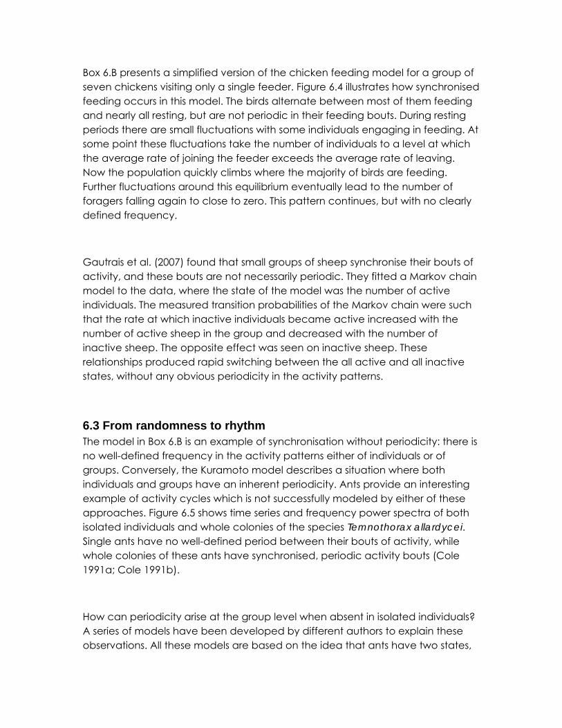
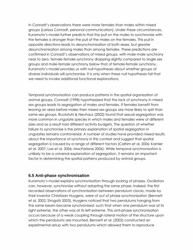
6.3 From randomness to rhythm The model in Box 6.B is an example of synchronisation without periodicity: there is no well-defined frequency in the activity patterns either of individuals or of groups. Conversely, the Kuramoto model describes a situation where both individuals and groups have an inherent periodicity. Ants provide an interesting example of activity cycles which is not successfully modeled by either of these approaches. Figure 6.5 shows time series and frequency power spectra of both isolated individuals and whole colonies of the species Temnothorax allardycei. Single ants have no well-defined period between their bouts of activity, while whole colonies of these ants have synchronised, periodic activity bouts (Cole 1991a; Cole 1991b).

How can periodicity arise at the group level when absent in isolated individuals? A series of models have been developed by different authors to explain these observations. All these models are based on the idea that ants have two states,

active and inactive. They further assume that encounters with active ants increase the probability of other active ants remaining active and/or the probability of inactive ants becoming active. As was shown in Box 6.B such processes can certainly create synchronization, but it is less clear how they generate periodicity.

(b)

Figure 6.5: Activity records for (a) three colonies of Leptothorax acervorum and (b) three isolated individual ants. One time unit is one minute. Reproduced from Cole (1991b)

An initial suggestion by Goss and Deneubourg (1988) was that after a bout of activity, inactive ants have an ‘unwakeable’ period where interactions with others do not result in them becoming active. Under this model, isolated individuals’ inactive bouts have a deterministic minimum time plus an exponentially distributed period until the start of the next active bout. In groups, this latter part of the inactivity bout can be interrupted by disturbance from other ants, whereby all ants are woken by the first ant coming out of its bout of

inactivity. As a result, the inactive bouts become equal to the length of the ‘unwakeable’ periods and the ‘unwakeable’ periods become synchronised. An alternative assumption is that active ants are ‘unsleepable’ with some minimum length of activity bouts (Cole & Cheshire 1996; Sole & Miramontes 1995; Sole et al. 1993). The effect in these models is similar to the ‘unwakeable’ model: although there was a minimum time between the start of activity bouts in isolated ants, the time between bouts has no well-defined period. When in groups, however, the ants became synchronised with the gaps between the starts of bouts determined by the ‘unsleepable’ periods. These observations are largely consistent with observations of real ants (figure 6.5).

Activity bouts within ant colonies are not always periodic. Franks et al. (1990) found that colonies of Leptothorax acervorum have synchronized, but not always periodic bouts of activity. Boi et al. (1999) found that periodicity was strongest amongst workers further from the entrance to the nest and was disturbed by the return of workers to the colony. They also found that activity originated in the centre of the nest, where the brood is kept, and spread outwards. In experiments where forager returns were prevented activity started first and lasted longer in the centre of the nest than at the nest entrance.

6.4 Why synchronise? Synchronised activities are beneficial to individuals in a range of situations. For example, sheep (Ruckstuhl 1999), deer (Conradt 1998) and other ungulates have synchronised bouts of feeding and digestion. By choosing to forage for food together, individuals reduce their probability of being attacked by a predator and increase their opportunity for information transfer (see chapters 2 and 3). Synchronised activity could be a requirement for the social cohesion which allows animals to benefit from being in a group (Conradt & Roper 2000).

Box 6.C describes a simple functional model of a pair of animals, each of which chooses between either resting or foraging for food. The model assumes that the benefit of foraging decreases with the nutritional state of an individual. There is a cost associated with foraging, which is smaller if both individuals forage simultaneously. Two key points arise from the analysis of this model. The first point is that the evolutionarily stable strategy is for the individuals to synchronise their actions, i.e. forage at the same time and rest at the same time, even when their

nutritional states are different (figure 6.7). The second point is that synchronisation of actions does not imply synchronisation of nutritional state. Instead, the individual with the lower nutritional state initiates foraging and the individual with higher nutritional state follows, because of the benefit it gains from foraging with a partner. Once the individual with higher nutritional state reaches a level of nutrition such that it no longer pays to forage, even with a partner, it will stop foraging. At this point the less

Box 6.C: State-based synchronisation.

Rands et al. (2003) proposed a model of a pair of foragers who, based on their own nutritional state and that of their partner, decide whether to forage for food or rest. Here, I present a simplified version of their model which captures the essential features of the argument they present. Assume that on each day an individual must decide between foraging and resting. Foraging incurs a cost c due to predation risk but also gives a benefit b/s where b is a constant and s is the nutritional state of the individual. The benefit in foraging thus decreases inversely proportional to nutrional state. Further assume that if an individual forages at the same time as its partner it gains benefit e from dilution of risk. Thus the payoff for foraging together with a partner is b/s-c+e and the payoff for foraging alone is b/s-c. We assume that resting incurs neither benefit nor cost.

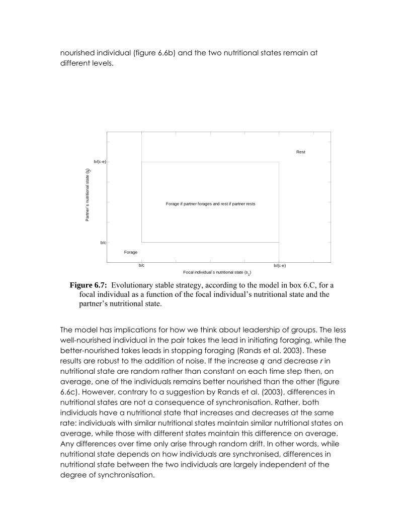
What strategy should an individual adopt? Let’s first consider the case where both individuals in the pair have the same nutritional state, s. In this case, if s<b/c then it always better to forage than to rest and both individuals will forage. If s>b/(c-e) then it always better to rest than to forage and both individuals will rest. For the intermediate values of b/c<s<b/(c-e) the maximum payoff is obtained if both individuals forage. However, if the focal individual forages and its partner rests then the focal individual will get the lowest of the possible payoffs. Furthermore, if both individuals are resting then swapping to foraging without the certainty that your partner will also swap is costly. The individuals thus do best if they co-ordinate their foraging and resting, i.e. they synchronise their active and inactive periods.

When b/c<s<b/(c-e), the evolutionary game defined in Table 1 is known as a co-ordination game (see chapter 10 for more about evolutionary games). There are two evolutionarily stable strategies to such games and deciding which strategy will evolve is not straightforward. On the one hand it is optimal, in terms of higher benefits, for both individuals to forage. On the other hand, unlike resting, foraging is prone to errors resulting from one individual failing to co-ordinate. Here, I resolve this co-ordination issue by assuming that in repeated iterations over a number of days, whenever b/c<s<b/(c-e) an individual will adopt the same behaviour as it adopted on the previous day. Nutritional state can now be made time dependent, i.e represented by st. Individuals rest whenever s>b/(c-e) or when b/c<s<b/(c-e) and both individuals rested on the previous day, resulting in a decrease in nutritional state i.e. st+1= st-r. Individuals forage whenever s<b/c or b/c<s<b/(c-e) and the individuals foraged on the previous day, resulting in an increase in nutritional state, i.e. st+1= st+q. Figure 6.6a shows the outcome of such dynamics. The individuals’ foraging bouts are periodic and synchronised and their nutritional states remain synchronised.

What happens if the individuals have different nutritional states, and ? Figure 6.7

summarises the conditions under which it is optimal for a focal individual to co-operate given its own nutritional state and the state of its partner. If we assume that the individuals are aware of

ts ,1 ts ,2

each others nutritional state, then if > both individuals will always forage when

and . Likewise, if and then both individuals rest. When

, it is best for individuals to co-ordinate. As in the case of identical

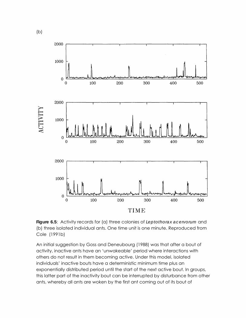
nutritional states, however, it is not immediately clear upon which activity they should co-ordinate. Assuming as before that co-ordination is determined by the individual’s previous action, the actions of the two individuals become synchronised (Figure 6.6b). Interestingly, nutritional state does not become synchronized. Instead, foraging is initiated by the individual the worst nutritional state while resting is initiated by the individual with the best nutritional state. As a result, the individual with lower nutrition never ‘catches up’ with its partner. If r and q are random variables, varying from day to day, instead of constant values the same pattern is seen (Figure 6.6b). In general, there is no correlation between the nutritional state of the individuals despite a strong synchrony in their foraging patterns.

ts ,1 ts ,2 cbs t /,2 <

)/(,1 ecbs t −< )/(,1 ecbs t −> cbs t /,2 >

cbssecb tt /,)/( ,2,1 >>−

(a)

10 20 30 40 50 60 70 80 90 100 1100

2

4

6

8

10

12

Day (t)

Nut

ritio

nal S

tate

(s)

Individual 1 forages

Individual 2 forages

(b)

10 20 30 40 50 60 70 80 90 100 1100

2

4

6

8

10

12

Day (t)

Nut

ritio

nal S

tate

(s)

Individual 1 forages

Individual 2 forages

(c)

100 200 300 400 500 600 700 800 900 10000

2

4

6

8

10

12

Day (t)

Nut

ritio

nal S

tate

(s)

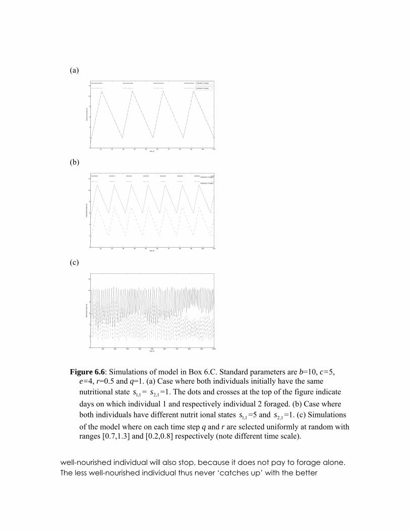
Figure 6.6: Simulations of model in Box 6.C. Standard parameters are b=10, c=5,

e=4, r=0.5 and q=1. (a) Case where both individuals initially have the same nutritional state = =1. The dots and crosses at the top of the figure indicate days on which individual 1 and respectively individual 2 foraged. (b) Case where both individuals have different nutrit ional states =5 and =1. (c) Simulations of the model where on each time step q and r are selected uniformly at random with ranges [0.7,1.3] and [0.2,0.8] respectively (note different time scale).

1,1s 1,2s

1,1s 1,2s

well-nourished individual will also stop, because it does not pay to forage alone. The less well-nourished individual thus never ‘catches up’ with the better

nourished individual (figure 6.6b) and the two nutritional states remain at different levels.

Forage

Rest

Forage if partner forages and rest if partner rests

Focal individual´s nutritional state (s1)

Par

tner

´s n

utrit

iona

l sta

te (s

2)

b/c

b/c b/(c-e)

b/(c-e)

Figure 6.7: Evolutionary stable strategy, according to the model in box 6.C, for a

focal individual as a function of the focal individual’s nutritional state and the partner’s nutritional state.

The model has implications for how we think about leadership of groups. The less well-nourished individual in the pair takes the lead in initiating foraging, while the better-nourished takes leads in stopping foraging (Rands et al. 2003). These results are robust to the addition of noise. If the increase q and decrease r in nutritional state are random rather than constant on each time step then, on average, one of the individuals remains better nourished than the other (figure 6.6c). However, contrary to a suggestion by Rands et al. (2003), differences in nutritional states are not a consequence of synchronisation. Rather, both individuals have a nutritional state that increases and decreases at the same rate: individuals with similar nutritional states maintain similar nutritional states on average, while those with different states maintain this difference on average. Any differences over time only arise through random drift. In other words, while nutritional state depends on how individuals are synchronised, differences in nutritional state between the two individuals are largely independent of the degree of synchronisation.

If each individual within a group has its own ‘ideal’ point in time they wish to perform an action then as group size increases the heterogeneity of rhythms within the group also increases. Conradt and Roper (2003) used a model to show that in most situations it is beneficial to group members that decisions about the timing of events are made by consensus rather than ‘despotically’. Their argument is based on the principle of ‘many wrongs’ presented in Box 4.B. It is better to time events according to the average preference, rather than adopting the preference of a single individual. Obtaining consensus between heterogeneous individuals is difficult, simply because different individuals want different things. Conradt and Roper (2007) develop an evolutionary game theory model of decision-making of groups of three or more members and show that over a wide range of conditions evolutionary stability of consensus can be obtained.

A prediction that arises both from Conradt and Roper’s functional models and from Kuramoto’s mechanistic model is that, if between-individual variation in the timing of events becomes too large then synchrony will break down. Conradt (1998) observed that male-only and female-only groups of red deer had more synchronised bouts of activity than mixed sex groups. This loss of synchrony could result from differences between males and females in the amount of food they need and the digestion time for this food (Ruckstuhl & Neuhaus 2002). Interestingly, within the mixed sex groups the female-female and male-male synchrony was much lower than that in the single sex groups. Similar observations have been made of alpine ibex (Ruckstuhl & Neuhaus 2001).

In terms of a functional explanation, desynchronisation in mixed sex groups could be attributed to male harassment of females, competition between males in the presence of females, or some other social conflict within the group (Conradt 1998). However, such desynchronisation is also explainable purely in terms of mechanisms. If the distribution of initial frequencies are bimodal, Kuramoto’s model predicts that those individuals with initial frequencies nearer to the mean initial frequency will synchronise, while those with initial frequencies further away from the mean will remain close to their initial frequency (Strogatz 2000). Thus a proportion of the males become more synchronized with the females, increasing the degree of male-female synchrony, above that of separate groups, while decreasing male-male synchrony.

In Conradt’s observations there were more females than males within mixed groups (Larissa Conradt, personal communication). Under these circumstances, Kuramoto’s model further predicts that the pull on the males to synchronise with the females is stronger than the pull of the males on the females. This pull in opposite directions leads to desynchronisation of both sexes, but greater desynchronisation among males than among females. These predictions are confirmed in Conradt’s observations of mixed groups, with male-male synchrony near to zero, female-female synchrony dropping slightly compared to single sex groups and male-female synchrony below that of female-female synchrony. Kuramoto’s model provides us with null hypotheses about whether groups of diverse individuals will synchronise. It is only when these null hypotheses fail that we need to invoke additional functional explanations.

Temporal synchronisation can produce patterns in the spatial organization of animal groups. Conradt (1998) hypothesized that the lack of synchrony in mixed sex groups leads to segregation of males and females. If females benefit from leaving an area before males then mixed sex groups are more likely to split than same sex groups. Ruckstuhl & Neuhaus (2002) found that sexual segregation was more common in ungulate species in which males and females were of different sizes and as a result had different activity budgets. The question of whether failure to synchronise is the primary explanation of spatial segregation in ungulates remains controversial. A number of studies have provided mixed results about the importance of synchrony in this context and suggest that spatial segregation is caused by a range of different factors (Calhim et al. 2006; Kamler et al. 2007; Loe et al. 2006; MacFarlane 2006). While temporal synchronisation is unlikely to be a universal explanation of segregation, it remains an important factor in determining the spatial patterns produced by animal groups.

6.5 Anti-phase synchronisation Kuramoto’s model explains synchronisation through locking of phases. Oscillators can, however, synchronise without adopting the same phase. Indeed, the first recorded observations of synchronisation between pendulum clocks, made by their inventor Christiaan Huygens, were of out of phase synchronisation (Bennett et al. 2002; Strogatz 2003). Huygens noticed that two pendulums hanging from the same beam became synchronised, such that when one pendulum was at its right extreme, the other was at its left extreme. This anti-phase synchronisation occurs because of a weak coupling through lateral motion of the structure upon which the pendulums are mounted. Bennett et al. (2002) constructed an experimental setup with two pendulums which allowed them to reproduce

Huygens’ findings. They developed a mathematical model to show that anti-phase synchronisation is the only stable outcome for this system provided there is sufficiently strong coupling between the pendulums. As in the Kuramoto model, synchronisation occurs even when the natural frequencies of the pendulums are slightly different.

An example of pairs or small groups of animals becoming anti-phase synchronised is sentinel behaviour. McGowan & Woolfenden (1989) observed small groups of Florida scrub jays and noted when each member engaged in vigilance, looking around for potential threats, and foraging, looking for food. They found that vigilance was co-ordinated, such that periods of vigilance overlapped less than expected than if the decision to become vigilant was independent of the behaviour of other individuals. One of the birds acted as a sentinel while the others fed. The periods of sentinel behaviour were out of phase with each other, reducing the probability that a predator could attack unnoticed.

A functional explanation of sentinel behaviour poses a challenge, because the individual keeping watch is losing the opportunity to forage for food. What is to stop the sentinel from cheating and skipping its turn to continue foraging instead? The dilemma here is similar to that of producers and scroungers (Box 3.B) and is a typical example of social parasitism (see chapter 10). Although the group would have the least risk of predation were individuals to take turns being sentinels, for each individual the incentive is to often skip their turn to keep watch. Bednekoff (1997) proposed a simple solution to this problem based on selfish sentinels. He considered how nutritional state should influence the relative costs and benefits to an individual of foraging and sentinel behaviour. Individuals that have just fed have a lower need for food and thus a greater incentive to take a safe position where they can keep watch. Bednekoff’s model predicted that if being sentinel provided extra safety compared to foraging and that if a sentinel detected a predator this information spread to foragers then co-ordinated sentinels was an evolutionarily stable behaviour.

Bednekoff & Woolfenden performed experiments on pairs of Florida scrub jays to test the plausibility of Bednekoff’s model. They found that when scrub jays were fed they spent less time feeding and more time acting as sentinels (Bednekoff & Woolfenden 2003). Furthermore, the partners of the fed individuals reduced their time acting as sentinels and foraged more (Bednekoff & Woolfenden 2006). In

pairs of scrub jays these responses can leads to a ‘seesaw’ synchronisation of feeding and sentinel behaviour. Individual A finds food and then begins to act as a sentinel, while individual B searches for food. When individual B has found food, its tendency to become a sentinel increases, while individual A’s tendency to feed increases. In this case, and unlike the model of in-phase synchronisation in Box 6.C, anti-phase synchronisation arises from and sustains differences in nutritional state.

Animals in larger groups also exhibit turn taking in sentinel behaviour. Meerkats forage by digging into the ground, in a manner that makes it impossible to observe what is going on around them. The meerkats usually forage in groups. When not digging, some individuals stand guard, looking around for potential predators. Clutton-Brock et al. (1999) observed that meerkats take turns in guarding when living in groups. If there was no guard then the probability that an individual would start guarding was twice as high as when there was a guard, and if two or more individuals happened to be guarding at the same time one of them would usually stop guarding relatively quickly. Turn taking was not in a consistent order, although individuals did not tend to take consecutive bouts of guarding. Like the scrub jays, an important factor in whether a meerkat would guard was whether it had been fed or not. Clutton-Brock et al. (1999) found that if they fed meerkats they would guard more often and forage less.

Clutton-Brock et al.’s (1999) experiments “provide no indication that the alternation of raised guarding depends on social processes more complex than the independent optimization of activity by individuals, subject to nutritional status and the presence (or absence) of an existing guard”. Bednekoff’s (1997) model provides an elegant mathematical demonstration of how this guard alternation can evolve. It also provides an extension of the seesaw concept and double pendulum anti-phase synchronisation to groups of more than two individuals. Simply by aiming to maximise their own survival individuals will move out of nutritional phase with each other, so that there is usually a single guard with a high nutritional level.