CHAPTER 6 1

CHAPTER 6CHAPTER 6GRAPHS

All the programs in this file are selected from

Ellis Horowitz, Sartaj Sahni, and Susan Anderson-Freed“Fundamentals of Data Structures in C”,Computer Science Press, 1992.

CHAPTER 6 2

Definition A graph, G=(V, E), consists of two sets:

a finite set of vertices(V), and a finite, possibly empty set of edges(E) V(G) and E(G) represent the sets of vertices and edges of

G, respectively Undirected graph

The pairs of vertices representing any edges is unordered e.g., (v0, v1) and (v1, v0) represent the same edge

Directed graph Each edge as a directed pair of vertices e.g. <v0, v1> represents an edge, v0 is the tail and v1 is the

head

(v0, v1) = (v1,v0)

<v0, v1> != <v1,v0>

CHAPTER 6 3

Examples for Graph0

1 2

3

0

1

2

0

1 2

3 4 5 6G1

G2G3

V(G1)={0,1,2,3} E(G1)={(0,1),(0,2),(0,3),(1,2),(1,3),(2,3)}V(G2)={0,1,2,3,4,5,6} E(G2)={(0,1),(0,2),(1,3),(1,4),(2,5),(2,6)}V(G3)={0,1,2} E(G3)={<0,1>,<1,0>,<1,2>}

complete undirected graph: n(n-1)/2 edgescomplete directed graph: n(n-1) edges

complete graph incomplete graph

CHAPTER 6 4

Complete Graph

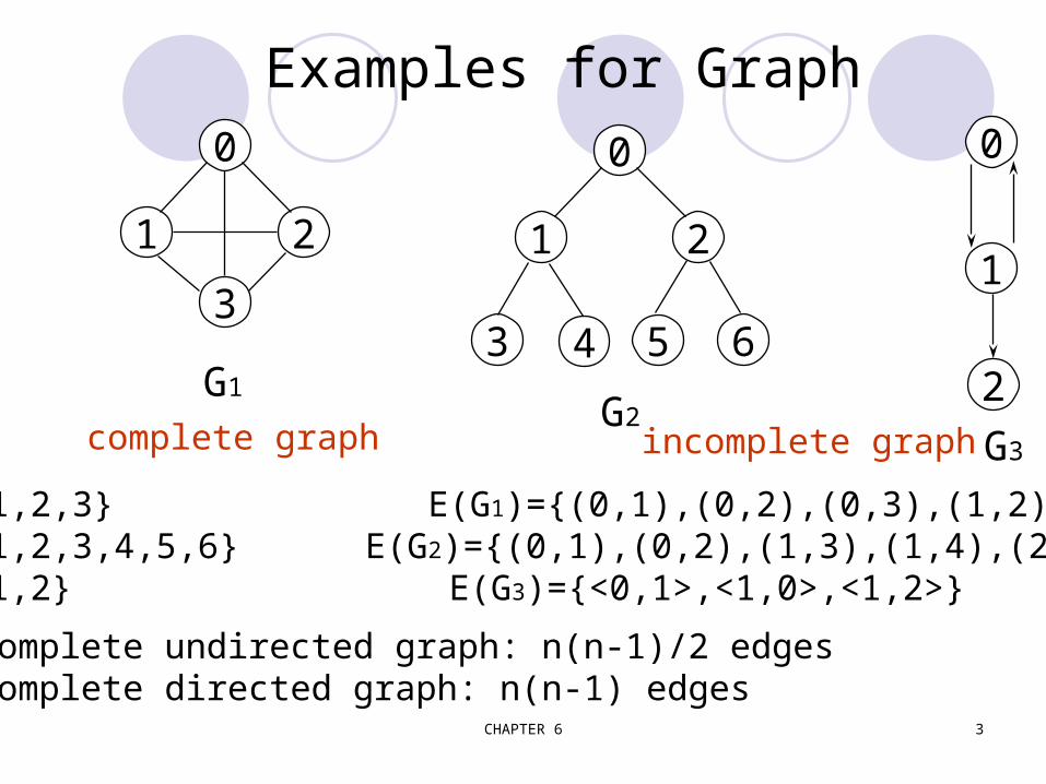
A complete graph is a graph that has the maximum number of edges for undirected graph with n vertices, the

maximum number of edges is n(n-1)/2 for directed graph with n vertices, the maximum

number of edges is n(n-1) example: G1 is a complete graph

CHAPTER 6 5

Adjacent and Incident

If (v0, v1) is an edge in an undirected graph, v0 and v1 are adjacent The edge (v0, v1) is incident on vertices v0 and v1

If <v0, v1> is an edge in a directed graph v0 is adjacent to v1, and v1 is adjacent from v0

The edge <v0, v1> is incident on v0 and v1

CHAPTER 6 6

0 2

1

(a)

2

1

0

3

(b)

*Figure 6.3:Example of a graph with feedback loops and a multigraph (p.260)

self edge multigraph:multiple occurrencesof the same edge

Figure 6.3

CHAPTER 6 7

A subgraph of G is a graph G’ such that V(G’) is a subset of V(G) and E(G’) is a subset of E(G)

A path from vertex vp to vertex vq in a graph G, is a sequence of vertices, vp, vi1, vi2, ..., vin, vq, such that (vp, vi1), (vi1, vi2), ..., (vin, vq) are edges in an undirected graph

The length of a path is the number of edges on it

Subgraph and Path

CHAPTER 6 8

0 0

1 2 3

1 2 0

1 2

3 (i) (ii) (iii) (iv) (a) Some of the subgraph of G1

0 0

1

0

1

2

0

1

2(i) (ii) (iii) (iv)

(b) Some of the subgraph of G3

分開單一

0

1 2

3

G1

0

1

2

G3

Figure 6.4: subgraphs of G1 and G3 (p.261)

CHAPTER 6 9

A simple path is a path in which all vertices, except possibly the first and the last, are distinct

A cycle is a simple path in which the first and the last vertices are the same

In an undirected graph G, two vertices, v0 and v1, are connected if there is a path in G from v0 to v1

An undirected graph is connected if, for every pair of distinct vertices vi, vj, there is a path from vi to vj

Simple Path and Style

CHAPTER 6 10

0

1 2

3

0

1 2

3 4 5 6G1

G2

connected

tree (acyclic graph)

CHAPTER 6 11

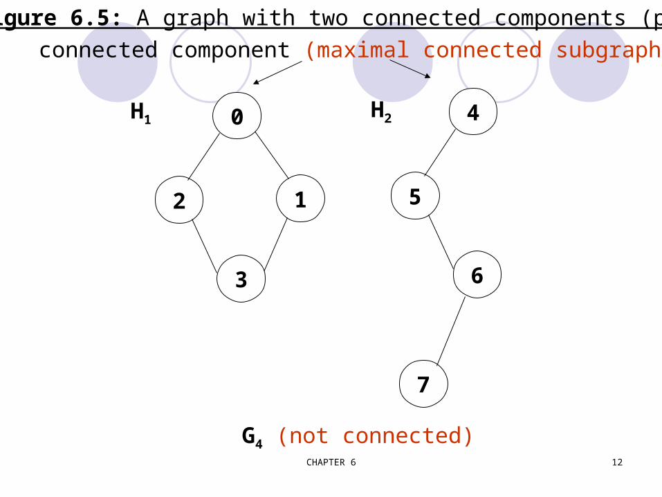
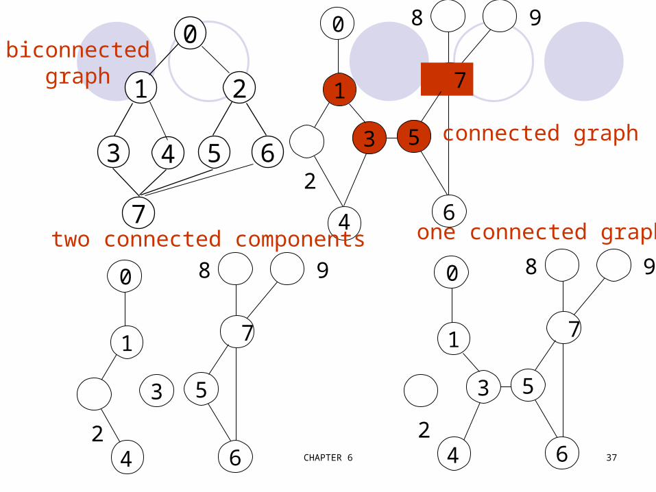
A connected component of an undirected graph is a maximal connected subgraph.

A tree is a graph that is connected and acyclic. A directed graph is strongly connected if there

is a directed path from vi to vj and also from vj to vi.

A strongly connected component is a maximal subgraph that is strongly connected.

Connected Component

CHAPTER 6 12

*Figure 6.5: A graph with two connected components (p.262)

1

0

2

3

4

5

6

7

H1 H2

G4 (not connected)

connected component (maximal connected subgraph)

CHAPTER 6 13

*Figure 6.6: Strongly connected components of G3 (p.262)

0

1

20

1

2

G3

not strongly connectedstrongly connected component

(maximal strongly connected subgraph)

CHAPTER 6 14

Degree The degree of a vertex is the number of edges incid

ent to that vertex For directed graph,

the in-degree of a vertex v is the number of edgesthat have v as the head

the out-degree of a vertex v is the number of edgesthat have v as the tail

if di is the degree of a vertex i in a graph G with n vertices and e edges, the number of edges is

e di

n

( ) /0

1

2

CHAPTER 6 15

undirected graph

degree0

1 2

3 4 5 6

G1 G2

3

2

3 3

1 1 1 1

directed graphin-degreeout-degree

0

1

2

G3

in:1, out: 1

in: 1, out: 2

in: 1, out: 0

0

1 2

3

33

3

CHAPTER 6 16

ADT for Graphstructure Graph is objects: a nonempty set of vertices and a set of undirected edges, where each

edge is a pair of vertices

functions: for all graph Graph, v, v1 and v2 Vertices Graph Create()::=return an empty graph Graph InsertVertex(graph, v)::= return a graph with v inserted. v has no

incident edge. Graph InsertEdge(graph, v1,v2)::= return a graph with new edge

between v1 and v2 Graph DeleteVertex(graph, v)::= return a graph in which v and all edges

incident to it are removed Graph DeleteEdge(graph, v1, v2)::=return a graph in which the edge (v1, v2)

is removed Boolean IsEmpty(graph)::= if (graph==empty graph) return TRUE else return FALSE List Adjacent(graph,v)::= return a list of all vertices that are adjacent to v

CHAPTER 6 17

常見的表示法

Adjacency matricesAdjacency listsAdjacency multilists

0

1 2

3

G1

2

1

0

G3

0

12

3

4

65

7

G4

CHAPTER 6 18

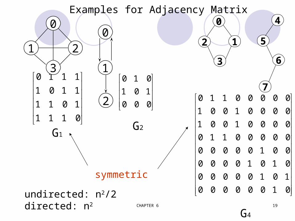
Adjacency Matrix Let G=(V,E) be a graph with n vertices. The adjacency matrix of G is a two-dimensional

n by n array, say adj_mat If the edge (vi, vj) is in E(G), adj_mat[i][j]=1 If there is no such edge in E(G), adj_mat[i][j]=0 The adjacency matrix for an undirected graph is sy

mmetric; the adjacency matrix for a digraph need not be symmetric If the matrix is sparse ?

大部分元素是 0e << (n^2/2)

CHAPTER 6 19

Examples for Adjacency Matrix

0

1

1

1

1

0

1

1

1

1

0

1

1

1

1

0

0

1

0

1

0

0

0

1

0

0

1

1

0

0

0

0

0

1

0

0

1

0

0

0

0

1

0

0

1

0

0

0

0

0

1

1

0

0

0

0

0

0

0

0

0

0

1

0

0

0

0

0

0

1

0

1

0

0

0

0

0

0

1

0

1

0

0

0

0

0

0

1

0

G1G2

G4

0

1 2

3

0

1

2

1

0

2

3

4

5

6

7

symmetric

undirected: n2/2directed: n2

CHAPTER 6 20

Merits of Adjacency Matrix

From the adjacency matrix, to determine the connection of vertices is easy

The degree of a vertex is For a digraph, the row sum is the

out_degree, while the column sum is the in_degree

adj mat i jj

n

_ [ ][ ]

0

1

ind vi A j ij

n

( ) [ , ]

0

1outd vi A i j

j

n

( ) [ , ]

0

1

CHAPTER 6 21

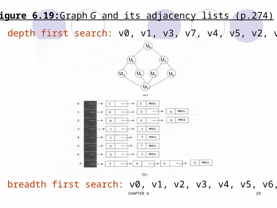
Adjacency lists

n 個 linked list 1

2 0

3 1 2

2 3 0

1 3 0

210

2

1

0

G3

0

1 2

3

G1

#define MAX_VERTICES 50

typedef struct node *node_ptr;

typedef struct node {

int vertex;

node_ptr link;

} node;

node_ptr graph[MAX_VERTICES];

int n = 0; /* number of nodes */

CHAPTER 6 22

Adjacency lists, by array

000

101

010

2

1

0

G3

1

2 0

0217754

6543210

CHAPTER 6 23

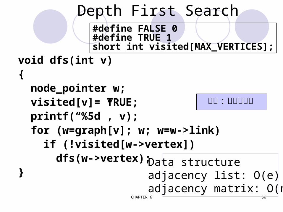
Interesting Operations

degree of a vertex in an undirected graph–# of nodes in adjacency list

# of edges in a graph–determined in O(n+e)

out-degree of a vertex in a directed graph–# of nodes in its adjacency list

in-degree of a vertex in a directed graph–traverse the whole data structure

CHAPTER 6 24

[0] 9 [8] 23 [16] 2[1] 11 [9] 1 [17] 5[2] 13 [10] 2 [18] 4[3] 15 [11] 0 [19] 6[4] 17 [12] 3 [20] 5[5] 18 [13] 0 [21] 7[6] 20 [14] 3 [22] 6[7] 22 [15] 1

1

0

2

3

4

5

6

7

0

1

2

3

45

6

7

node[0] … node[n-1]: starting point for verticesnode[n]: n+2e+1node[n+1] … node[n+2e]: head node of edge

Compact Representation

CHAPTER 6 25

tail head column link for head row link for tail

Figure 6.11: Alternate node structure for adjacency lists (p.267)

CHAPTER 6 26

0 1 2

2 NULL

1

0

1 0 NULL

0 1 NULL NULL

1 2 NULL NULL

0

1

2

0

1

0

1

0

0

0

1

0

Figure 6.12: Orthogonal representation for graph G3(p.268)

CHAPTER 6 27

Adjacency multilists

m vertex1 vertex2 list1 list2

0 2 N2 N3

N1

0 3 NIL N4

N2

1 2 N4 N5

N3

1 3 NIL N5

N4

2 3 NIL NILN5

0 1 N1 N3

N0

0

1 2

3

G1

typedef struct edge *edge_ptr;Typedef struct edge {

int marked;int vertex1;int vertex2;edge_ptr path1;edge_ptr path2;

} edge;edge_ptr graph[MAX_VERTICES];

CHAPTER 6 28

Some Graph Operations

TraversalGiven G=(V,E) and vertex v, find all wV, such that w connects v. Depth First Search (DFS)

preorder tree traversal Breadth First Search (BFS)

level order tree traversal

Connected ComponentsSpanning Trees

CHAPTER 6 29

*Figure 6.19:Graph G and its adjacency lists (p.274)

depth first search: v0, v1, v3, v7, v4, v5, v2, v6

breadth first search: v0, v1, v2, v3, v4, v5, v6, v7

CHAPTER 6 30

Depth First Search

void dfs(int v){ node_pointer w; visited[v]= TRUE; printf(“%5d”, v); for (w=graph[v]; w; w=w->link) if (!visited[w->vertex]) dfs(w->vertex);}

#define FALSE 0#define TRUE 1short int visited[MAX_VERTICES];

Data structureadjacency list: O(e)adjacency matrix: O(n2)

例如 : 老鼠走迷宮

CHAPTER 6 31

Breadth-First Searchvoid bfs(int v) {

node_ptr w;queue_ptr front, rear;front=rear=NULL;printf(“%5d”,v);visited[v]=TRUE;addq(&front, &rear, v);while(front) {

v = deleteq(&front);for(w=graph[v]; w; w=w->link)

if(!visited[w->vertex]) {printf(“%5d”, w->vertex);addq(&front, &rear, w->vertex);visited[w->vertex] = TRUE;

}}

}}

typedef struct queue *queue_ptr;typedef struct queue {

int vertex;queue_ptr link;

};void addq(queue_ptr *, queue_ptr *, int);Int deleteq(queue_ptr);

adjacency list: O(e)adjacency matrix: O(n2)

例如 : 地毯式搜索

CHAPTER 6 32

Connected component

Is it a connected graph? BFS(v) or DFS(v)

Find out connected component

void connected(void){int i;for (i=0;i<n;i++){

if(!visited[i]){dfs(i);printf(“\n”);

}}

adjacency list: O(n+e)adjacency matrix: O(n2)

CHAPTER 6 33

Spanning Tree

A spanning tree is a minimal subgraph G’, such that V(G’)=V(G) and G’ is connected

Weight and MST3 1 2

2 3 0

1 3 0

210

0

1 2

3

G1

0

1 2

3

0

1 2

3

DFS(0) BFS(0)

CHAPTER 6 34

Spanning Trees

Either dfs or bfs can be used to create a spanning tree When dfs is used, the resulting spanning tree is

known as a depth first spanning tree When bfs is used, the resulting spanning tree is

known as a breadth first spanning tree

While adding a nontree edge into any spanning tree, this will create a cycle

CHAPTER 6 35

DFS VS BFS Spanning Tree

0

1 2

3 4 5 6

7

0

1 2

3 4 5 6

7

DFS Spanning BFS Spanning

0

1 2

3 4 5 6

7 nontree edgecycle

CHAPTER 6 36

Biconnected components

Definition: Articulation point ( 關節點 ) 原文請參閱課本 如果將 vertex v 以及連接的所有 edge 去除 , 產生 graph

G’, G’ 至少有兩個 connected component, 則 v 稱為 articulation point

Definition: Biconnected graph 定義為無 Articulation point 的 connected graph

Definition: Biconnected component Graph G 中的 Biconnected component H, 為 G 中最大

的 biconnected subgraph; 最大是指 G 中沒有其他 subgraph 是 biconnected 且包含入 H

CHAPTER 6 37

1

3 5

6

0 8 9

7 2

4

connected graph

1

3 5

6

0 8 9

7 2

4

1

3 5

6

0 8 9

7 2

4

two connected components one connected graph

0

1 2

3 4 5 6

7

biconnectedgraph

CHAPTER 6 38

biconnected component: a maximal connected subgraph H(no subgraph that is both biconnected and properly contains H)

1

3 5

6

0 8 9

7 2

4

1

0

1

3

2

4

3 5

8

7

9

7

5

6

7

biconnected components為何沒有任一個邊可能存在於兩個或多個biconnected component 中 ?

CHAPTER 6 39

dfn() and low()

Observation 若 root 有兩個以上 child, 則為 articulation point 若 vertex u 有任一 child w, 使得 w 及 w 後代無法透過 ba

ck edge 到 u 的祖先 , 則為 articulation point

low(u): u 及後代 , 其 back edge 可達 vertex 之最小 dfn() low(u) = min{ dfn(u), min{low(w)|w 是 u 的 child}, min{dfn

(w)|(u,w) 是 back edge}}

u: articulation pointlow(child) dfn(u)

CHAPTER 6 40

Find biconnected component of a connected undirected graphby depth first spanning tree

8 9

1

4 0

3 0 5 3 5

4 61 6

9 8 9 8

7 7

3

4 5

7

6

9 8

2

0

1

0

6

7

1 5

2

4

3

(a) depth first spanning tree (b)

2 2

dfndepthfirst

number

nontreeedge

(back edge)

nontreeedge

(back edge)

Why is cross edge impossible?

If u is an ancestor of v then dfn(u) < dfn(v).

CHAPTER 6 41

*Figure 6.24: dfn and low values for dfs spanning tree with root =3(p.281)

Vertax 0 1 2 3 4 5 6 7 8 9

dfn 4 3 2 0 1 5 6 7 9 8

low 4 0 0 0 0 5 5 5 9 8

CHAPTER 6 42 8 9

3

4 5

7

6

9 8

2

0

1

6

7

1 5

2

4

3

vertex dfn low child low_child low:dfn0 4 4 (4,n,n) null null null:41 3 0 (3,4,0) 0 4 4 3 2 2 0 (2,0,n) 1 0 0 < 23 0 0 (0,0,n) 4,5 0,5 0,5 0 4 1 0 (1,0,n) 2 0 0 < 15 5 5 (5,5,n) 6 5 5 5 6 6 5 (6,5,n) 7 5 5 < 67 7 5 (7,8,5) 8,9 9,8 9,8 7 8 9 9 (9,n,n) null null null, 99 8 8 (8,n,n) null null null, 8

CHAPTER 6 43

*Program 6.5: Initializaiton of dfn and low (p.282)

void init(void) { int i; for (i = 0; i < n; i++) { visited[i] = FALSE; dfn[i] = low[i] = -1; } num = 0; }

CHAPTER 6 44

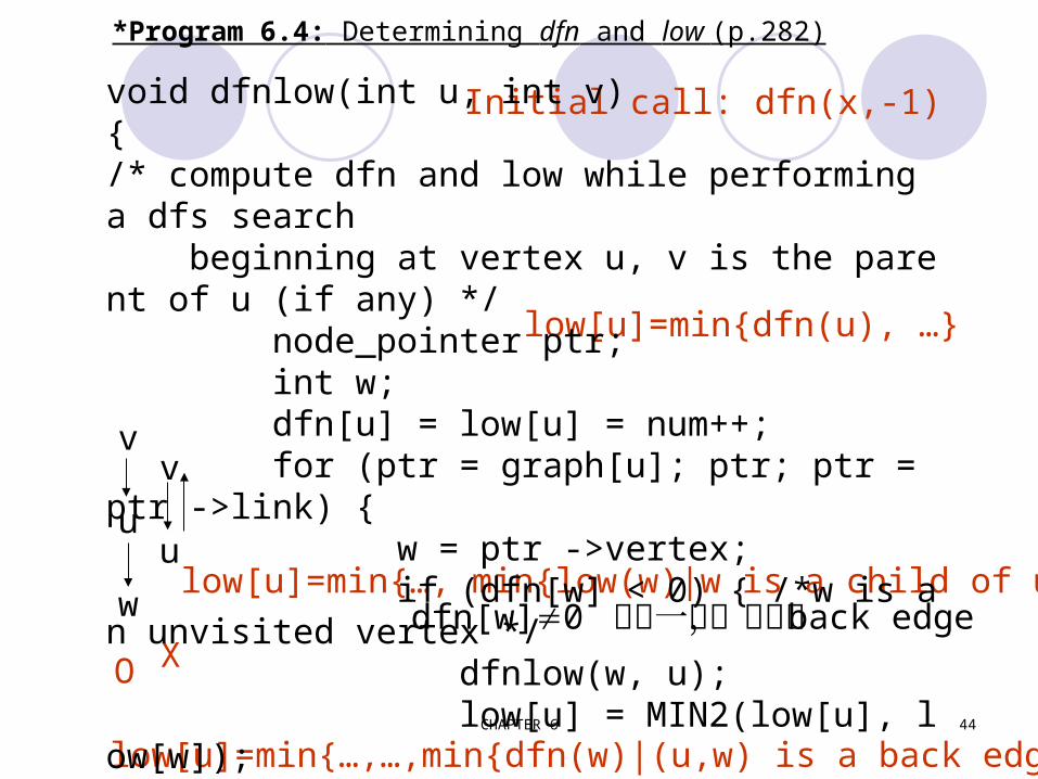
*Program 6.4: Determining dfn and low (p.282)

Initial call: dfn(x,-1)

low[u]=min{dfn(u), …}

low[u]=min{…, min{low(w)|w is a child of u}, …}

low[u]=min{…,…,min{dfn(w)|(u,w) is a back edge}

dfn[w]0 非第一次，表示藉 back edge

v

u

w

v

u

XO

void dfnlow(int u, int v){/* compute dfn and low while performing a dfs search beginning at vertex u, v is the parent of u (if any) */ node_pointer ptr; int w; dfn[u] = low[u] = num++; for (ptr = graph[u]; ptr; ptr = ptr ->link) { w = ptr ->vertex; if (dfn[w] < 0) { /*w is an unvisited vertex */ dfnlow(w, u); low[u] = MIN2(low[u], low[w]); } else if (w != v) low[u] =MIN2(low[u], dfn[w] ); }}

CHAPTER 6 45

*Program 6.6: Biconnected components of a graph (p.283)

low[u]=min{dfn(u), …}

(1) dfn[w]=-1 第一次(2) dfn[w]!=-1非第一次，藉 back edge

void bicon(int u, int v){/* compute dfn and low, and output the edges of G by their biconnected components , v is the parent ( if any) of the u (if any) in the resulting spanning tree. It is assumed that all entries of dfn[ ] have been initialized to -1, num has been initialized to 0, and the stack has been set to empty */ node_pointer ptr; int w, x, y; dfn[u] = low[u] = num ++; for (ptr = graph[u]; ptr; ptr = ptr->link) { w = ptr ->vertex; if ( v != w && dfn[w] < dfn[u] ) add(&top, u, w); /* add edge to stack */

CHAPTER 6 46

if(dfn[w] < 0) {/* w has not been visited */ bicon(w, u); low[u] = MIN2(low[u], low[w]); if (low[w] >= dfn[u] ){ articulation point printf(“New biconnected component: “); do { /* delete edge from stack */ delete(&top, &x, &y); printf(“ <%d, %d>” , x, y); } while (!(( x = = u) && (y = = w))); printf(“\n”); } } else if (w != v) low[u] = MIN2(low[u], dfn[w]); } }

low[u]=min{…, …, min{dfn(w)|(u,w) is a back edge}}

low[u]=min{…, min{low(w)|w is a child of u}, …}

CHAPTER 6 47

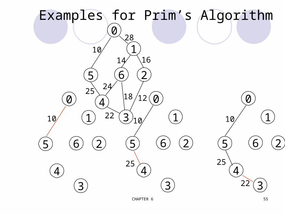
Minimum-cost spanning trees (MST) in a given graph

A minimum-cost spanning tree is a spanning tree of least cost

Design strategy – greedy method Kruskal’s algorithm

Edge by edge Prim’s algorithm

Span out from one vertex Sollin’s algorithm

Hint: Construct from connected components Leave as a homework

CHAPTER 6 48

Greedy Strategy

An optimal solution is constructed in stages At each stage, the best decision is made at this

time Since this decision cannot be changed later,

we make sure that the decision will result in a feasible solution

Typically, the selection of an item at each stage is based on a least cost or a highest profit criterion

CHAPTER 6 49

Kruskal’s Idea

Build a minimum cost spanning tree T by adding edges to T one at a time

Select the edges for inclusion in T in nondecreasing order of the cost

An edge is added to T if it does not form a cycle

Since G is connected and has n > 0 vertices, exactly n-1 edges will be selected

CHAPTER 6 50

Examples for Kruskal’s Algorithm

0

1

2

34

5 6

0

1

2

34

5 6

28

16

121824

22

25

1014

0

1

2

34

5 6

10

0 5

2 3

1 6

1 2

3 6

3 4

4 6

4 5

0 1

10

12

14

16

18

22

24

25

28 6/9

CHAPTER 6 51

0

1

2

34

5 6

10

12

0

1

2

34

5 6

10

12

14

0

1

2

34

5 6

10

12

14 16

0 5

2 3

1 6

1 2

3 6

3 4

4 6

4 5

0 1

10

12

14

16

18

22

24

25

28 + 3 6

cycle

CHAPTER 6 52

0 5

2 3

1 6

1 2

3 6

3 4

4 6

4 5

0 1

10

12

14

16

18

22

24

25

28

0

1

2

34

5 6

10

12

14 16

22

0

1

2

34

5 6

10

12

14 16

22

25

4 6

cycle

+

cost = 10 +25+22+12+16+14

CHAPTER 6 53

Kruskal’s algorithmEdge by edgeO(e log e)Algorithm:

T={};While ((T contains less than n-1 edges) &&(E not empty)){

choose an edge (v,w) from E of lowest cost;delete (v,w) from E;if((v,w) does not create a cycle in T)

add(v,w) to T;else

discard(v,w);}If(T contains fewer than n – 1 edges)

printf(“No spanning tree\n”);

CHAPTER 6 54

Prim’s algorithmBegins from a vertexO(n2)Algorithm:

T={};TV = {0}; /* start with vertex 0 and no edges */While (T contains fewer than n-1 edges){

let(u,v) be a least cost edge s.t. u in TV and v not in TV;if (there is no such edge)

break;add v to TV;add (u,v) to T;

}If (T contains fewer than n-1 edges)

printf(“No spanning tree\n”);

CHAPTER 6 55

Examples for Prim’s Algorithm

0

1

2

34

5 6

0

1

2

34

5 6

10

0

1

2

34

5 6

1010

25 25

22

0

1

2

34

5 6

28

16

121824

22

25

1014

CHAPTER 6 56

0

1

2

34

5 6

10

25

22

12

0

1

2

34

5 6

10

25

22

12

16

0

1

2

34

5 6

10

25

22

12

1614

0

1

2

34

5 6

28

16

121824

22

25

1014

CHAPTER 6 57

Sollin’s Algorithm

0

1

2

34

5 6

10

0

22

12

1614

0

1

2

34

5 6

10

22

12

14

0

1

2

34

5 6

0

1

2

34

5 6

28

16

121824

22

25

1014

vertex edge0 0 -- 10 --> 5, 0 -- 28 --> 11 1 -- 14 --> 6, 1-- 16 --> 2, 1 -- 28 --> 02 2 -- 12 --> 3, 2 -- 16 --> 13 3 -- 12 --> 2, 3 -- 18 --> 6, 3 -- 22 --> 44 4 -- 22 --> 3, 4 -- 24 --> 6, 5 -- 25 --> 55 5 -- 10 --> 0, 5 -- 25 --> 46 6 -- 14 --> 1, 6 -- 18 --> 3, 6 -- 24 --> 4

{0,5}

5 4 0 125 28

{1,6}

1 216 281

6 3 6 418 24

CHAPTER 6 58

Is there a path? How short it can be?

Single source/ All destinations Nonnegative edge costs General weights

All-pairs shortest pathTransitive closure

CHAPTER 6 59

Single source all destinationsDijkstra’s algorithm

A spanning tree againFor nonnegative edge costs (Why?)Start from a vertex v, greedy methoddist[w]: the shortest length to w through S

v

u

w

length(<u,w>)

dist[w]

dist[u]

CHAPTER 6 60

*Figure 6.29: Graph and shortest paths from v0 (p.293)

V0 V4V1

V5V3V2

50 10

20 10 15 20 35 30

15 3

45

(a)

path length1) v0 v2 102) v0 v2 v3 253) v0 v2 v3 v1 454) v0 v4 45

(b)

Single Source All Destinations

Determine the shortest paths from v0 to all the remaining vertices.

CHAPTER 6 61

Example for the Shortest Path

0

1 23

4

5

67

SanFrancisco Denver

Chicago

Boston

NewYork

Miami

New Orleans

Los Angeles

300 1000

8001200

1500

1400

1000

9001700

1000250

0 1 2 3 4 5 6 70 01 300 02 1000 800 03 1200 04 1500 0 2505 1000 0 900 14006 0 10007 1700 0

Cost adjacency matrix

CHAPTER 6 62

43

5

1500

250

43

5

1500

250

1000

選 5 4到 3由 1500改成 1250

4

5

250

6900

4到 6由改成 1250

4

5

250

7 1400

4到 7由改成 1650

4

5

250

6900

7 1400

3

1000

選 6

4

5

250

6900

7 1400

1000

4-5-6-7比 4-5-7長

(a) (b) (c)

(d) (e) (f)

CHAPTER 6 63

4

5

250

6900

7 1400

3

1000

選 3

4

5

250

6900

7 1400

3

1000

2 1200

4到 2由改成 2450

4

5

250

6900

7 1400

3

1000

2 1200

選 7

4

5

250

7 1400

0

4到 0由改成 3350

(g) (h)

(i)(j)

CHAPTER 6 64

Example for the Shortest Path(Continued)

Iteration S VertexSelected

LA[0]

SF[1]

DEN[2]

CHI[3]

BO[4]

NY[5]

MIA[6]

NO

Initial -- ---- + + + 1500 0 250 + +

1 {4} 5 + + + 1250 0 250 1150 16502 {4,5} 6 + + + 1250 0 250 1150 16503 {4,5,6} 3 + + 2450 1250 0 250 1150 16504 {4,5,6,3} 7 3350 + 2450 1250 0 250 1150 16505 {4,5,6,3,7} 2 3350 3250 2450 1250 0 250 1150 16506 {4,5,6,3,7,2} 1 3350 3250 2450 1250 0 250 1150 16507 {4,5,6,3,7,2,1}

(a)(b) (c) (d)

(e)(f)

(g)(h)

(i)(j)

CHAPTER 6 65

Data Structure for SSAD

#define MAX_VERTICES 6int cost[][MAX_VERTICES]= {{ 0, 50, 10, 1000, 45, 1000}, {1000, 0, 15, 1000, 10, 1000}, { 20, 1000, 0, 15, 1000, 1000}, {1000, 20, 1000, 0, 35, 1000}, {1000, 1000, 30, 1000, 0, 1000}, {1000, 1000, 1000, 3, 1000, 0}};int distance[MAX_VERTICES];short int found{MAX_VERTICES];int n = MAX_VERTICES;

adjacency matrix

CHAPTER 6 66

shortest()

Void shortestpath(int v, int cost[][MAX_VERTICES], int dist [], int n, int found[]){

int i,u,w;for (i=0;i<n;i++) {

found[i]=FALSE;dist [i] = cost[v][i];

}found[v]=TRUE;dist [v]=0;for(i=0;i<n-2;i++){

u=choose(dist,n,found);found[u]=TRUE;for(w=0;w<n;w++)

if(dist [u]+cost[u][w] < dist [w])dist [w] = dist [u]+cost[u][w];

}} O(n2)

CHAPTER 6 67

Single source all destinationsBellmanFord algorithm

For general weightsPath has at most n-1 edges, otherwise…distk[u]: from v to u, has at most k edges ]}}][[][{min],[min{][ 11 uilengthidistudistudist k

i

kk

0

1

2

3

4

5

6

6

5

5

1

-1

-2

-2

-1

3

33405310

5405310

7425310

455330

5560

6543210

CHAPTER 6 68

BellmanFord()

Void BellmanFord(int n, int v) {

int i,k;for (i =0;i<n;i++)

dist[i] = length[v][i];for(k=2;k<=n-1;k++)

for(each u s.t. u!=v and u has at least one incoming edge)for(each <i,u> in the graph)

if(dist([u]>dist[i]+length[i][u])dist[u]=dist[i]+length[i][u];

}

O(n^3)

CHAPTER 6 69

All-Pairs shortest paths

執行 n 次 single source all destinations algo.Dynamic programming strategy

利用 recursive formula 來表示 好好地 implement recursive formula, 用 table 輔助

Ak[i][j] ≡ shortest length from i to j through no intermediate vertex greater than k

A-1[i][j] = length[i][j]Ak[i][j] = min{Ak-1[i][j], Ak-1[i][k]+ Ak-1[k][j], k≥0

CHAPTER 6 70

AllLengths()

Void AllLength(int n){

int i,j,k;for(i=0;i<n;i++)

for(j=0;j<n;j++)a[i][j] = length[i][j];

for(k=0;k<n;k++)for(i=0;i<n;i++)

for(j=0;j<n;j++)if((a[i][k]+a[k][j])<a[i][j])

a[i][j] = a[i][k]+a[k][j];}

O(n^3)

0 1

2

6

4

211

3

CHAPTER 6 71

Transitive closure

Definition: transitive closure matrix, A+

A+[i][j] = 1, if there’s a path of length > 0 from i to j A+[i][j] = 0, otherwise

Definition: reflexive transitive closure matrix, A* A*[i][j] = 1, if there’s a path of length >= 0 from i to j A*[i][j] = 0, otherwise

O(n^3), by AllLengths() O(n^2), an undirected graph, by connected chec

k

CHAPTER 6 72

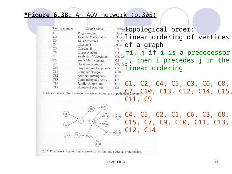
Activity on Vertex (AOV) Network definitionA directed graph in which the vertices represent tasks or activities and the edges represent precedence relations between tasks.predecessor (successor)vertex i is a predecessor of vertex j iff there is a directed path from i to j. j is a successor of i.partial ordera precedence relation which is both transitive (i, j, k, ij & jk => ik ) and irreflexive (x xx).acyclic grapha directed graph with no directed cycles

CHAPTER 6 73

*Figure 6.38: An AOV network (p.305)

Topological order:linear ordering of verticesof a graphi, j if i is a predecessor ofj, then i precedes j in thelinear ordering

C1, C2, C4, C5, C3, C6, C8,C7, C10, C13, C12, C14, C15, C11, C9

C4, C5, C2, C1, C6, C3, C8,C15, C7, C9, C10, C11, C13,C12, C14

CHAPTER 6 74

*Program 6.13: Topological sort (p.306)

for (i = 0; i <n; i++) { if every vertex has a predecessor { fprintf(stderr, “Network has a cycle. \n “ ); exit(1); } pick a vertex v that has no predecessors; output v; delete v and all edges leading out of v from the network;}

CHAPTER 6 75

*Figure 6.39:Simulation of Program 6.13 on an AOV network (p.306)

v0 no predecessordelete v0->v1, v0->v2, v0->v3 v1, v2, v3 no predecessor

select v3delete v3->v4, v3->v5

select v2delete v2->v4, v2->v5

select v5

select v1delete v1->v4

CHAPTER 6 76

Issues in Data Structure Consideration

Decide whether a vertex has any predecessors.–Each vertex has a count.

Decide a vertex together with all its incident edges.

–Adjacency list

CHAPTER 6 77

*Figure 6.40:Adjacency list representation of Figure 6.30(a)(p.309)

0 1 2 3 NULL

1 4 NULL

1 4 5 NULL

1 5 4 NULL

3 NULL

2 NULL

V0

V1

V2

V3

V4

V5

v0

v1

v2

v3

v4

v5

count linkheadnodes

vertex linknode

CHAPTER 6 78

*(p.307)

typedef struct node *node_pointer;typedef struct node { int vertex; node_pointer link; };typedef struct { int count; node_pointer link; } hdnodes;hdnodes graph[MAX_VERTICES];

CHAPTER 6 79

*Program 6.14: Topological sort (p.308)

O(n)

void topsort (hdnodes graph [] , int n){ int i, j, k, top; node_pointer ptr; /* create a stack of vertices with no predecessors */ top = -1; for (i = 0; i < n; i++) if (!graph[i].count) {no predecessors, stack is linked through graph[i].count = top; count field top = i; }for (i = 0; i < n; i++) if (top == -1) { fprintf(stderr, “\n Network has a cycle. Sort terminated. \n”); exit(1);}

CHAPTER 6 80

O(e)

O(e+n)

Continued} else { j = top; /* unstack a vertex */ top = graph[top].count; printf(“v%d, “, j); for (ptr = graph [j]. link; ptr ;ptr = ptr ->link ){ /* decrease the count of the successor vertices of j */ k = ptr ->vertex; graph[k].count --; if (!graph[k].count) { /* add vertex k to the stack*/ graph[k].count = top; top = k; } } } }

CHAPTER 6 81

Activity on Edge (AOE) Networks

directed edge–tasks or activities to be performed

vertex–events which signal the completion of certain activities

number–time required to perform the activity

CHAPTER 6 82

*Figure 6.41:An AOE network(p.310)

concurrent

CHAPTER 6 83

Application of AOE Network

Evaluate performance–minimum amount of time

–activity whose duration time should be shortened

–…

Critical path–a path that has the longest length

–minimum time required to complete the project

–v0, v1, v4, v7, v8 or v0, v1, v4, v6, v8 (18)

CHAPTER 6 84

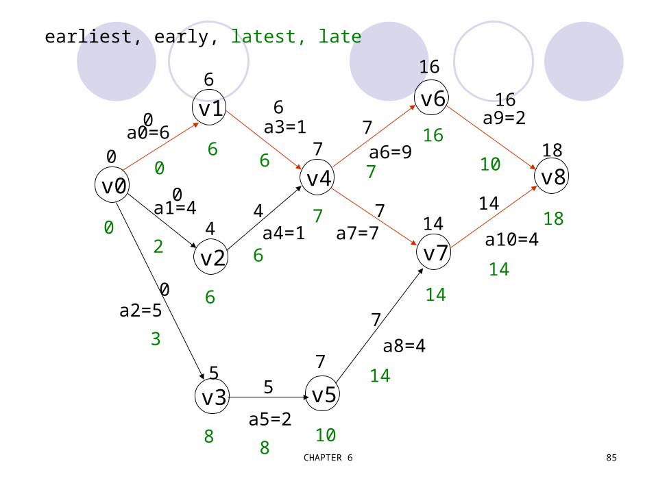
other factorsEarliest time that vi can occur

–the length of the longest path from v0 to vi

–the earliest start time for all activities leaving vi

–early(6) = early(7) = 7Latest time of activity

–the latest time the activity may start without increasing the project duration

–late(5)=8, late(7)=7

Critical activity–an activity for which early(i)=late(i)

–early(7)=late(7)

late(i)-early(i)–measure of how critical an activity is

–late(5)-early(5)=8-5=3

CHAPTER 6 85

v0

v1

v2

v3

v4

v5

v6

v7

v8

a0=6

a1=4

a2=5

a3=1

a4=1

a5=2

a6=9

a7=7

a9=2

a10=4

a8=4

earliest, early, latest, late

0

0

6

6

77

16

16

18

0

44 7

1414

0

55

7

7

0

06

6

7

7

16

10

18

2

6

6

14

14

14

108

8

3

CHAPTER 6 86

Determine Critical Paths

Delete all noncritical activitiesGenerate all the paths from the start to finish vertex.

CHAPTER 6 87

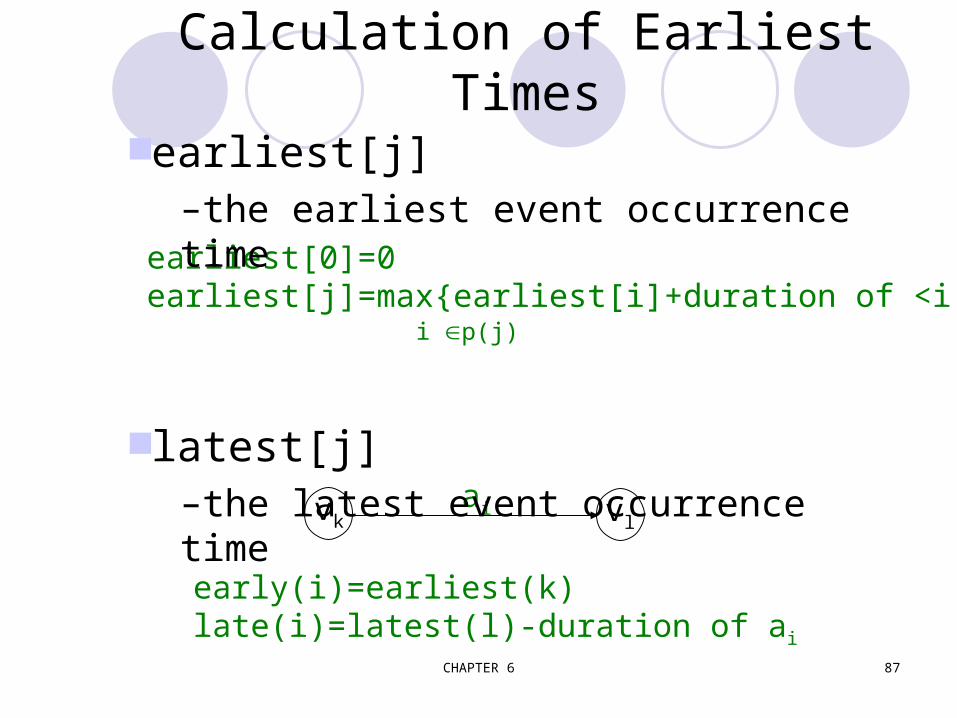
Calculation of Earliest Times

vk vlai

early(i)=earliest(k)late(i)=latest(l)-duration of ai

earliest[0]=0earliest[j]=max{earliest[i]+duration of <i,j>}

i p(j)

earliest[j]–the earliest event occurrence time

latest[j]–the latest event occurrence time

CHAPTER 6 88

vi1

vi2

vin

.

.

.

vjforward stage

if (earliest[k] < earliest[j]+ptr->duration) earliest[k]=earliest[j]+ptr->duration

CHAPTER 6 89

*Figure 6.42:Computing earliest from topological sort (p.313)

v0

v1

v2

v3

v4

v6

v7

v8

v5

CHAPTER 6 90

Calculation of Latest Timeslatest[j]

the latest event occurrence time

latest[n-1]=earliest[n-1]latest[j]=min{latest[i]-duration of <j,i>}

i s(j) vi1

vi2

vin

.

.

.

vj backward stage

if (latest[k] > latest[j]-ptr->duration) latest[k]=latest[j]-ptr->duration

CHAPTER 6 91

*Figure 6.43: Computing latest for AOE network of Figure 6.41(a)(p.314)

CHAPTER 6 92

*Figure 6.43(continued):Computing latest of AOE network of Figure 6.41(a)(p.315)

latest[8]=earliest[8]=18 latest[6]=min{earliest[8] - 2}=16 latest[7]=min{earliest[8] - 4}=14 latest[4]=min{earliest[6] - 9;earliest[7] -7}= 7 latest[1]=min{earliest[4] - 1}=6 latest[2]=min{earliest[4] - 1}=6 latest[5]=min{earliest[7] - 4}=10 latest[3]=min{earliest[5] - 2}=8 latest[0]=min{earliest[1] - 6;earliest[2]- 4; earliest[3] -5}=0(c)Computation of latest from Equation (6.4) using a reverse topological order

CHAPTER 6 93

*Figure 6.44:Early, late and critical values(p.316)

Activity Early Late Late-Early

Critical

a0

a1

a2

a3

a4

a5

a6

a7

a8

a9

a10

0006457771614

02366877101614

02302300300

YesNoNoYesNoNoYesYesNoYesYes

CHAPTER 6 94

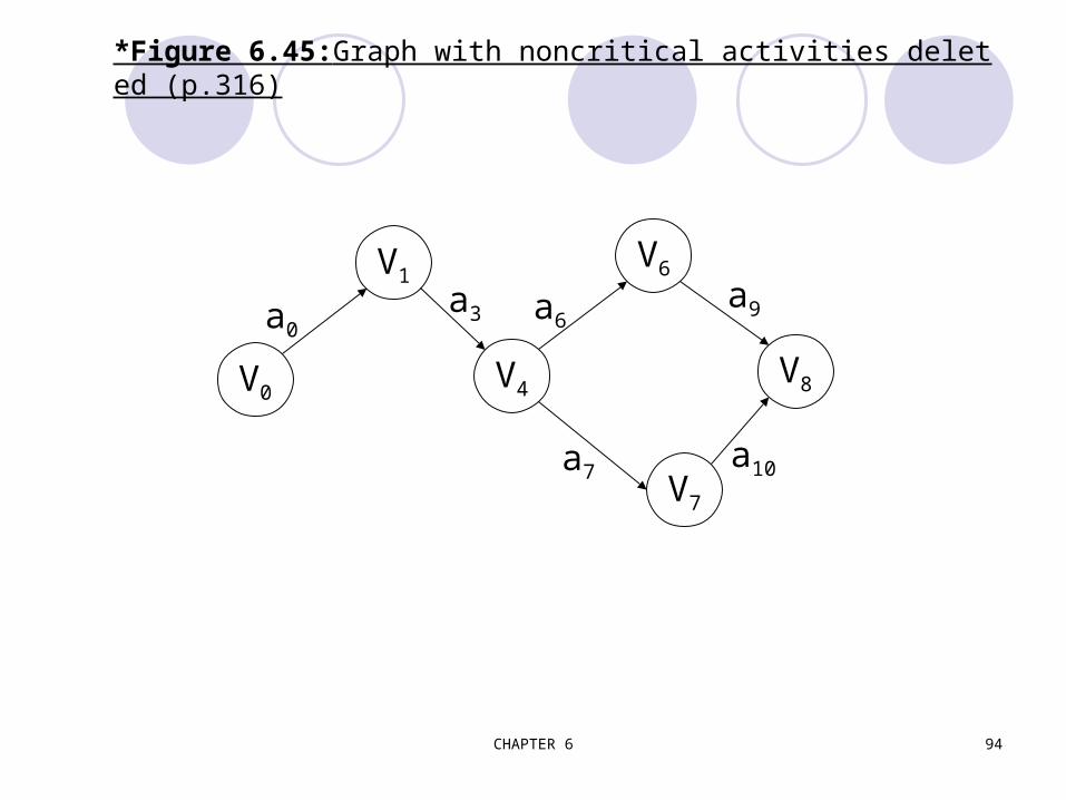
*Figure 6.45:Graph with noncritical activities deleted (p.316)

V0V4

V8

V1V6

V7

a0a3 a6

a7a10

a9

CHAPTER 6 95

*Figure 6.46: AOE network with unreachable activities (p.317)

V0

V3

V1

V5

V2

V4

a0

a1

a2

a3

a5 a6

a4

earliest[i]=0

CHAPTER 6 96

*Figure 6.47: an AOE network(p.317)

V5 V8 V9

a10=5 a13=2

V2 V4 V7a4=3 a9=4

V1 V3 V6

a2=3 a6=4

V0

a12=4

a11=2a8=1

a7=4

a5=3a3=6

a0=5

a1=6

start finish