Random Processes 7.1 Statistical Description A random process or stochastic process is a function that maps all elements of a sample space into a collection or ensemble of time functions called sample functions. The term sample function is used for the time function corresponding to a particular realization of the random process, which is similar to the designation of outcome for a particular realization of a random variable. A random process is governed by probabilistic laws, so that different observations of the time function can differ because a single point in the sample space maps to a single sample function. The value of a random process at any given time t cannot be predicted in advance. I f a process is not random it is called nonrandom or deterministic. As in the treatment of random phenomena earlier, it is convenient to consider the particular realization, of an observed random process, to be determined by random selection of an element from a sample space S. This implies that a particular element 5 E S is selected according to some random choice, with the realization of the random process completely determined by this random choice. To represent the time dependence and the random dependence, a random process is written as a function of two variables as X(t, s) t with trepresenting the time dependence and s the randomly chosen element of S. As was the case for random variables, for which the notation indicating the dependence on s was often suppressed, i.e., X was used instead of X(s), a random process will be written as X(t) instead of X(f, s) when it is not necessary to use the latter notation for clarity. A precise definition of a random process is as follows: (a) Let 5 be a nonempty set, (b) Let P( ) be a probability measure defined over subsets of S, and (c) To each se S let there correspond a time function X(t, s). 238 7.1 Statistical Description 239 Then this probability system is called a random process. This definition is simply a more precise statement of the earlier comments that the actual realization of the random process is determined by a random selection of an element from S. The collection of all possible realizations {X(t, s): se S} = {X(t, sj, X(t, s 2 ),...} is called the ensemble of functions in the random process, where the elements in this set are the sample functions. (As given, S is countable, but 5 may be uncountable.) Sometimes it is useful to denote the possible values of t by indicating that they are elements of another set, T. The ensemble of functions in the random process would then be given as {X(t t s): re T f seS}. To help clarify these ideas, several examples of random processes will now be considered. With the Bernoulli random variable X(t k ) = X kt which takes on the values 0 and 1, and with t k a time index, {X(t k ,s):k = ..., -2, -1,0,1,2,.,., 5 = 0,1} or simply {X k : k = ..., -2, -1,0,1,2,...} (where the 5 variation is suppressed) is the ensemble of functions in a Bernoulli random process. There is an infinite number of sample functions in this ensemble. Also, if y * = £ x k Y N is a binomial random variable, and for N a time index the binomial counting random process is expressed as Y(t)= Y N , NT<t<(N + l)T, N = 1, 2 , . . . , where T is the observation period. There is an infinite number of sample functions in the ensemble of the binomial random process. A typical sample function for the binomial random process [(x lt x 2 ,.. .)- (1,0,0,1,1,1,0,1,...) and (y,,y 2 ,...) = (1,1,1,2,3,4,4, 5,...)] is shown in Fig. 7.1.1. As shown, the process may increment by 1 only at the discrete times t k = kT t fc= 1,2, Y(t) 5 • . 4 • , 3 • , 2 • . 1 - | o I L j 1 1 i i i * - > . 0 T 2T 3T 4T 5T 6T 7T 8T 9T Fig. 7.1.1. Sample function for a binomial random process.
Transcript
Random Processes
7.1 Statistical Description
A random process or stochastic process is a function that maps all elements of a sample space into a collection or ensemble of time functions called sample functions. The term sample function is used for the time function corresponding to a particular realization of the random process, which is similar to the designation of outcome for a particular realization of a random variable. A random process is governed by probabilistic laws, so that different observations of the time function can differ because a single point in the sample space maps to a single sample function. The value of a random process at any given time t cannot be predicted in advance. I f a process is not random it is called nonrandom or deterministic.
As in the treatment of random phenomena earlier, it is convenient to consider the particular realization, of an observed random process, to be determined by random selection of an element from a sample space S. This implies that a particular element 5 E S is selected according to some random choice, with the realization of the random process completely determined by this random choice. To represent the time dependence and the random dependence, a random process is written as a function o f two variables as X(t, s)t with trepresenting the time dependence and s the randomly chosen element o f S. As was the case for random variables, for which the notation indicating the dependence on s was often suppressed, i.e., X was used instead of X(s), a random process wil l be written as X(t) instead of X( f , s) when it is not necessary to use the latter notation for clarity.
A precise definition of a random process is as follows:
(a) Let 5 be a nonempty set, (b) Let P( ) be a probability measure defined over subsets of S, and (c) To each se S let there correspond a time function X(t, s).
238
7.1 Statistical Description 239
Then this probability system is called a random process. This definition is simply a more precise statement of the earlier comments that the actual realization of the random process is determined by a random selection of an element from S.
The collection of all possible realizations {X(t, s): se S} = {X(t, sj, X(t, s2),...} is called the ensemble o f functions in the random process, where the elements in this set are the sample functions. (As given, S is countable, but 5 may be uncountable.) Sometimes it is useful to denote the possible values of t by indicating that they are elements of another set, T. The ensemble of functions in the random process would then be given as {X(tts): re TfseS}.
To help clarify these ideas, several examples of random processes wi l l now be considered. With the Bernoulli random variable X(tk) = Xkt which takes on the values 0 and 1, and with tk a time index, {X(tk,s):k = . . . , - 2 , - 1 , 0 , 1 , 2 , . , . , 5 = 0,1} or simply {Xk: k = . . . , - 2 , - 1 , 0 , 1 , 2 , . . . } (where the 5 variation is suppressed) is the ensemble of functions in a Bernoulli random process. There is an infinite number of sample functions in this ensemble. Also, i f
y * = £ xk
YN is a binomial random variable, and for N a time index the binomial counting random process is expressed as Y(t)= YN, NT<t<(N + l)T, N = 1, 2 , . . . , where T is the observation period. There is an infinite number of sample functions in the ensemble of the binomial random process. A typical sample function for the binomial random process [(xlt x2,.. . ) -(1 ,0 ,0 ,1 ,1 ,1 ,0 ,1 , . . . ) and ( y , , y 2 , . . . ) = (1 ,1 ,1 ,2 ,3 ,4 ,4 , 5 , . . . ) ] is shown in Fig. 7.1.1. As shown, the process may increment by 1 only at the discrete times tk = kTt fc= 1,2,
Y(t)
5 • .
4 • ,
3 • ,
2 • .
1 - |
o I L j 1 1 i i i * - > .
0 T 2T 3T 4T 5T 6T 7T 8T 9T
Fig. 7.1.1. Sample function for a binomial random process.
240 7 Random Prtcenes
X(t) 5 • r •
4 . .
3 - I
2 - j —
1 • |
0 I LJ 1 i 1 ' • —i 1 1 — t 0 T 2T 3T 4T ST 6T 7T 8T 97
Fig, 7,1 J , Sample /unction f o r i Poisson random process.
Another counting process is the Poisson random process, which counts the number o f events o f some type (e.g., photons in a photomultiplier tube) that are obtained from some initial time (often ( - 0) until time t. The number o f events obtained i n a fixed interval o f time is described by a Poisson random variable. I f N, denotes the number of arrivals before time t, then this process is given as X(t) = Nt. A typical sample function for the Poisson random process is shown in Fig. 7.1.2. As can be seen in this figure, the Poisson random process differs from the binomial random process in that it can be incremented by 1 at any time and is not limited to the discrete times tk = kT, k = 1,2,
A random process called a random telegraph signal can be obtained from the Poisson random process by taking the value at t ~ 0 to be either + 1 or - 1 with equal probability, and changing to the opposite value at the points where the Poisson process is incremented. A typical sample function of this random process is shown in Fig. 7.1.3. This telegraph signal can change values at any time.
o
- l
Y(t)
• • ' 0 T 2T 3T 4T 5T 6T 7T 8T 9T
Fig. 7.1.3. Sample function for a random telegraph signal.
7.1 Statistical Description 241
Another example of a random process is the sine wave random process given as
X(t)= Vs in ( f l / + 9 )
where the amplitude V may be random (which is the case for amplitude modulation), the frequency Cl may be random (which is the case for frequency modulation), the phase 0 may be random (which is the case for phase modulation), or any combination of these three parameters may be random. For the random process X(t) - cos(cu0' + 0 ) , where a>0 is a constant and 8 is a uniform phase with fB(8) = 1/(2TT), 0 ^ 8 < 2ir, there is an infinite number of sample functions (all of the same frequency and maximum value, with different phase angles), since there is an infinite number of values in the interval from 0 to 2ir. The random process for a simple binary communication scheme is X( t) = cos(w 0/ + 0 ) , where 0 has the value 6 = 0 or Q = TT, and consists o f the two sample functions x(t, S|) = cos(ft>00 and x(t, s2) = cos(o*0( + 7r). This binary phase modulation or, as it is commonly called, phase shift keying is the most efficient (yields the smallest probability of error) binary communication scheme.
The last example o f a random process is a noise waveform which might distort the received waveform in a communication system. A typical sample function is shown in Fig. 7.1.4. The noise waveforms are greatly affected
X(t)
Fig. 7.1.4. Sample function for a noise random process.
by the filtering and other operations performed on the transmitted waveforms, so it is difficult to draw a general waveform. The most common assumption concerning the type of noise random process is that it is Gaussian.
Since a random process is a function of two variables, t and s, either or both of these may be chosen to be fixed. With the fixed values denoted by
242 7 Random Processes
a subscript, these descriptions are
(a) X{t, s)-X{t) is a random process. (b) X(th s)~X(tt) = Xtl is a random variable. (c) X(t, Sj) = x(t, Sj) is a deterministic time function or sample function. (d) X(t,, Sj) - x(t>, Sj) is a real number.
For case (b) the time is fixed, so the possible values are the values that X(t) can take on at this one instant in time, which is completely equivalent to the description of a one-dimensional random variable. Thus, X{tt) is a random variable and can be described by a probability density function. Similar interpretations hold for the other cases.
Both parameters, t and s, of a random process may be either discrete or continuous. I f the possible values X(t) can take on are a discrete set of values, X{t) is said to be a discrete random process, whereas i f the possible values are a continuum of values, X{t) is said to be a continuous random process. The Bernoulli, binomial, Poisson, and telegraph random processes are discrete random processes, and the sine wave and noise random processes are continuous random processes. I f only values at the time instants < i , * j , . . . , t k t . . . are of interest, the random process has a discrete parameter or is designated as a discrete time random process (unless a parameter such as time is explicitly stated, the terms continuous and discrete describe the range of the real numbers the random process can take on). Such random processes are common in sampled data systems. I f time takes on a continuum of values, the random process has a continuous parameter or is a continuous time random process. The Bernoulli and binomial random processes are discrete time random processes, while the Poisson, telegraph, sine wave, and noise random processes are continuous time random processes.
The complete statistical description of a general random process can be infinitely complex. I n general, the density function of X(tt) depends on the value o f I f X{t) is sampled at N times, X T = X ( r 2 ) , . . . . X(tN)) is a random vector with joint density function that depends o n t l t t 2 , . . . , t N . A suitable description can in theory be given by describing the joint density function of X (or joint probability mass function) for all N and for all possible choices of tlt t2t..., tN. Such extremely general random process characterizations normally cannot be easily analyzed, so various simplifying assumptions are usually made. Fortunately, these simplifying assumptions are reasonable in many situations of practical interest. Random processes can be specified in several ways:
(a) Processes for which the rule for determining the density function is stated directly, e.g., the Gaussian random process
(b) Processes consisting of a deterministic time function with parameters that are random variables, e.g., the sine wave random process
7.2 Statistical Averages 243
(c) Operations on known random processes, e.g., filtering (d) Specification of the probability of a finite number of sample functions
The most common simplifying assumption on random processes is that they satisfy some type o f definition of stationarity. The concept of stationar-ity for a random process is similar to the idea of steady state in the analysis of the response of electrical circuits. I t implies that the statistics of the random process are, in some sense, independent of the absolute value of time. This does not imply that the joint statistics of X^) and X(t2) are independent of the relative times tt and t2, since for most random processes, as *! approaches t2tX(t2) becomes more predictable from the value o f X(t,). This type of behavior is readily satisfied, however, by allowing the dependence on time of these joint statistics to depend only on the difference between the two times, not on the precise value o f either of the times.
The first type of stationarity considered is the strongest type. The statement that a random process is stationary i f its statistical properties are invariant with respect to time translation is strict sense stationarity. Precisely stated, the random process X(t, s) is strict sense stationary i f and only if, for every value of N and for every set of time instants {t, € T, i -1,2,..., N}
FxOO.XUj) X ( l , v ) ( * ! , X 2 , . . . , XN) = F x ( , 1 + T ) i X ( , l + T ) X ( f N + * ) ( * l , * 2 , • • •» *N)
(7.1.1)
holds true for all values of x , , x 2 , . . . , xN and all T such that (f, + T ) G T for all i . This definition is simply a mathematical statement o f the property, which has already been stated, that the statistics depend only on time differences. Such differences are preserved i f all time values are translated by the same amount r.
The statistics of the Bernoulli random process do not change with time, so the Bernoulli random process is strict sense stationary, whereas the statistics o f the binomial and the Poisson process do change with time and they are nonstationary.
Strict sense stationarity is sometimes unnecessarily restrictive, since most of the more important results for real-world applications of random processes are based on second-order terms, or terms involving only two time instants. A weaker definition of stationarity involving the first and second moments w i l l be given shortly.
7.2 Statistical Averages
I t is often difficult to prove that a process is strict sense stationary, but proof of nonstationarity can at times be easy. A random process is
244 7 Random Processes
nonstationary i f any of its density functions (or probability functions) or any of its moments depend on the precise value of time.
Example 7.2.1. Consider the sine wave process with random amplitude given as
X ( f ) - Y cos(a>0r) - o o < t < c c
where w 0 is a constant frequency and V is a random variable uniformly distributed from 0 to 1, i.e.,
/ v ( y ) = l O s y ^ l
= 0 otherwise
The mean of the random process, where the expectation is over the random variation ( in this case Y), is obtained as
E[X(t)] = E[Yco8(«oO]- f y<Ms(w9t)fY(y)dy^ f y cos(o)0t)(\) dy J -oo JO
= COS(Q)OO f ydy=icos(a> 0 r ) Jo
where t is a constant with respect to the integration. Since the first moment is a function o f time, the process is nonstationary, O
Now consider the sine wave process with random phase.
Example 7.2.2. Consider the sine wave process given as
X(t) = c o s ( w 0 ' + 0 ) -co < r < oo
where again w 0 is a constant and the density function of 8 is
= 0 otherwise
H i e mean of X(t) is obtained as
E[X(t)] = £ [ c o s ( w o r + 0 ) ] = cos(o>0t+B)M$)dd J—oo
= I [cos(<M) co&(6)-sin(«,0 sin(0)]{j^j dB j I " « -2 i r | S-2ff1
= — cos(o» 0r) sin(fl) +s in(w 0 ( ) cos(0)\ 2ir L 9-o I e-o J
= ~ [cos(a) 0()(0 - 0) + s i n ( o i 0 ( ) ( l - D ] - 0 • 2 IT
7.2 Statistical Averages 245
Example 7.2.2 in itself does not prove or disprove that X{t) ~ cos(wor + 0 ) is stationary. That this random process is stationary is shown in Example 7.2.3.
Example 7.2.3. The sine wave random process of Example 7.2.2 is shown to be strict sense stationary by first observing that
0 = c o s " 1 [ X ( r , ) ] - a , o r 1 or 0 = 2 7 r - c o s " , [ X ( r 1 ) ] - f t i o i 1
From Example 3.3.2, the density function of X ( r , ) is obtained as
A ( i , ) ( * i ) = X - ^ - 1 ^ x , £ 1 « v 1 - x\
= 0 otherwise
Since neither this density function nor the density function for X{tt + r) depends on f,,
fx(tl)(x1)=fx(tl+T}(xl)
for all T and f,. Knowledge that X ( i , ) = x , specifies the value of the random variable 0 and correspondingly the sample function of the random process X{t). Given that X ( / , ) = x , , the value a, that wi l l be observed at time f, is therefore not random, but depends only on x t and the time difference ( i , - f i ) , and is given as
a, = cos[ft>0(i, - (,) + c o s " ' ( * i ) ] or a, = cos[w 0 ( ' f - ' i ) + 2TT - c o s " ' ( x i ) ]
The conditional density function of X(tt) given X(t%) is then
fxiu)\XiU){x,Ixt) = S(Xi -a,) i = 2, 3 , . . . , N
and does not depend on the time origin. Also, the conditional density function of X ( ( , + T) given X ( ( I + T ) ,
fxu,+T)\xitt+T)(Xt I * , ) = 8(x, - a,) all T and (, i = 2 , 3 , . . . , N
does not depend on the time origin. Thus for
X T ( t ) = ( X ( r , ) , X ( r 2 ) X(tN))
and
X T ( t + T ) = ( X ( r I + T),JV(r 2 + T ) , . . . , A ' ( r w + T ) )
it follows that
N /x(o(x)=/x( , , ) (x 1 ) n 5 ( x i - a i ) = / X ( t + T ) ( x )
(-2
which shows that X(t) is strict sense stationary. •
246 7 Random Process**
The complete set of joint and marginal density (or probability) functions give a complete description o f a random process, but they are not always available. Further, they contain more information than is often needed. Much of the study of random processes is based on a second-order theory, for which only the joint statistics applicable for two different instants of time are needed. These statistics are adequate for computing mean values of power (a second-order quantity, since it is based on the mean square value). The frequency spectra are also adequately described by these second-order statistics. An important random process that is completely described by second-order statistics is the Gaussian random process.
A situation where the second-order statistics are useful can be observed by evaluating the mean square value of the random output of the linear system shown in Fig. 7.2.1. The random output of the linear system is
X(t) ^ h(t)
Y(t) . h(t)
Fig. 7.2.1. Linear system with random input.
obtained in terms of the convolution integral of the random input and the impulse response o f the system as
Y X O - [ X(u)h(t-u)du J - 0 0
The mean square value is then obtained as
E [ y 2 ( t ) ] = B[[J X(u)h(t-u)du
= E { \ C ° J" X(u)X(v)h(t-u)h{t-v)dudv}
Talcing the expectation inside the double integration and associating it with the random quantity yields
E[Y2{t)] = f I E[X(u)X(v)]h(t-u)h(t~v) dudv J -co J —oo
The term E[X(u)X(v)] in this mean square value is a fundamental quantity in the consideration of random processes. I t is called the autocorrelation function of the random process X{t) and is defined, for the time instants r, and * 2 , as
As can be seen, the autocorrelation function o f the input to a linear system is needed to compute the mean square value o f the output.
Closely related to the autocorrelation function is the covariance function, which is a direct generalization of the definition of covariance. The covariance function is defined as
^ ( ' , , ( 2 ) = Cov[A-( / 1 ) ,A ' ( ( 2 ) ] = £ { [ X ( / I ) - H ( X ( r 1 ) ) ] [ X ( t 2 ) - £ ( A ' ( r 2 ) ) ] }
= Rx(tut2)-E[X(tl)]E[X(t2)]
= RMltt2)-mx(ti)mx(t2) (7.2.2)
where mx(t) = E[X(t)] is the mean function. The covariance function for a zero mean random process is identical to the autocorrelation function.
Example 7.2.4. Consider the sine wave process of Example 7.2.2 where X(t) = cos(io0t + &) w i t h / e ( 0 ) = l / ( 2 i r ) , 0=s 8<2n. The autocorrelation is given as
which is expressed in terms of only one integral, since there is only the one random variable 0 , as
RxUi, t2)= ( cos(oj0tl + e)cos{(o0t2+e)(~\ de
Jo \ 2 i r /
1 f 2 w
= — lcos((0otI+a>ot1 + 28) + cos(a>ot2-a/Qtl)]de
= £ c o s [ f t > o ( ' 2 - r i ) ]
where the trigonometric identity cos(A) cos(B) = [cos(A + B) + c o s ( A - B ) ] / 2 was used to help evaluate the integral. (The first term in the integral becomes the integral of a cosine over two periods, which is zero, while the second term does not involve 8 and yields 2TT times the constant value.) •
I n Example 7.2.4 Rx(tt, ' 2 ) depends only on the difference between the two time instants, t 2 - t x . Strict sense stationarity, which states that density or probability functions are invariant under translations of the time axis, implies that for a strict sense stationary random process the autocorrelation function depends only on the difference between t2 and (,. The converse of this is not necessarily true; i.e., the autocorrelation function depending only on time differences does, not necessarily imply strict sense stationarity (for an important class of random processes, Gaussian random processes, the converse is true, however). An example in which the autocorrelation
248 7 Random Processes
function depends only on the time difference and the process is not strict sense stationary is now given.
Example 7.2.5. Consider the random process X(t) with the sample functions
x(r, s,) - cos(i) x(r, s2) = -cos(f)
x( t, s3) ~ sin( r) x( t, 5 « ) = -sin( t)
which are equally likely. It can readily be determined that
mxU) = E[X(t)]=\ix(t,st) = 0 4 ( - i
and
Rx{ti>t2) = E[X(tl)X(t2)]=\ t X ( i l f i , ) X ( i A , 5 l ) » ^ c o s ( i 3 - i 1 )
which illustrates that the autocorrelation function depends only on t 2 - t x . That X(t) is not strict sense stationary can be shown by observing that at U = 0
fxWM * J a ( x , + n + J * ( x , ) + l * ( x , - 1 )
and at t2~ tx + r = 7r/4
or
/x ( l I >(* l )?* /x( l l +r>(Xl ) • As stated previously, a large part of the study of random processes is
built on the study of the autocorrelation function and related functions [the mean function mx(t) is also important in such studies]. For such analyses, only a form of stationarity which guarantees that the functions actually used depend on time differences is really needed. This form is considerably weaker than strict sense stationarity and leads to the definition of wide sense stationarity.
A random process X(t) is wide sense stationary i f the mean function mx(t) = E[X(t)] does not depend on t [mx(t) is a constant] and Rx(tx, t2) = Rx(T) is a function only o f r = t 2 - t x . I f X{t) is wide sense stationary, Rx(r) = E[X(t)X(t+T)] for all (.
7.2 Statistical Averages 249
The random process of Example 7.2.5, which has four sample functions, is wide sense stationary even though it is not strict sense stationary.
I t was shown in Section 4.4 that a linear combination of Gaussian random variables is a Gaussian random variable. I n a similar manner, the random variables X , , X2,..., XN are jointly Gaussian i f and only i f
is a Gaussian random variable for any set of g,'s. Now i f X{t) is a random process and
gU)X(t)dt (7.2.3)
where g(f) is any function such that Y has finite second moment, then X(t) is a Gaussian random process i f and.only i f Y is a Gaussian random variable for every g(t).
A direct consequence o f this is that the output of a linear system is a Gaussian random process i f the input is a Gaussian random process. To show that this is true, consider the output of a linear system with impulse response A(f) and input X(t) which is a Gaussian random process. The output is given as
Y(t) = [ h(t~u)X(u)du J -co
which is a Gaussian random process i f
Z=\ g{t)Y{t)dt J—OS
is a Gaussian random variable for all g(t). Substituting for Y(t) and interchanging the order of integration yields
Z = J g U )[\ H { t ~ u ) X ( u ) d u] d t
= j [| gU)h(t-u) dt^X(u)du = j g'(u)X{u)du
where
« ' ( « ) = I g{t)h{t-u)dt
Since X(t) is a Gaussian random process Z is a Gaussian random variable
250 7 Random Processes
for all g'(t), and thus, since Z is a Gaussian random variable, Y(t) is a Gaussian random process.
Another consequence of the definition of a Gaussian random process, given in Eq. (7.2.3), is that i f X(t) is a Gaussian random process the N random variables X{tx)yX(t2),..-,X(tN) are jointly Gaussian random variables [have an N-dimensional Gaussian density function as given in Eq. (4.4.1)]. This is shown by using
* ( 0 B ! * 8 ( » - ' i )
in Eq. (7.2.3), Frequently this property is used as the definition of a Gaussian random process; i.e., a Gaussian random process is defined as a random process for which the N random variables X ( * i ) , X ( f 2 ) , . . . , X(tN) are jointly Gaussian random variables for any N and any f,, ( 2 , . . . , tN. Even though this statement is straightforward, it is easier to prove that the output of a linear system is a Gaussian random process i f the input is a Gaussian random process by using the definition given here rather than using this last property.
The Gaussian random process is important for essentially the same reasons as Gaussian random variables; i t is appropriate for many engineering models or, using the central limit theorem, i f i t is obtained from the contributions of many quantities, e.g., electron movement. I n addition, analytical results are more feasible for the Gaussian random process than most other random processes. Just as a Gaussian random variable is specified by the mean and the variance, a Gaussian random process is specified by knowledge of the mean function mx(t) and the covariance function Kx{tu t2) [or equivalently by the mean function and the autocorrelation function Rx(ti,t2)].
I f X ( f ) is wide sense stationary, mx{t) = mxt a constant, and RX(T) is a function only o f the time difference r=t2-ty. From Eq. (7.2.2), Kx(T) also depends only on the time difference. Since the two functions that specify a Gaussian random process do not depend on the time origin (only on time difference), strict sense stationarity is also satisfied. Thus, wide sense stationarity implies strict sense stationarity for a Gaussian random process.
I n general, strict sense stationarity implies wide sense stationarity, since wide sense stationarity involves only the first two moments. The converse is not necessarily true; i.e., wide sense stationarity does not necessarily imply strict sense stationarity for a general random process, although the converse is true for the special case of a Gaussian random process.
Example 7.2.6. I f X(t) is a stationary Gaussian random process with mx(t) = 0 and Rx(T) = sin(7TT)/(7rT), the covariance matrix of the Gaussian
7.2 Statistical Averages 251
random vector X T = (X(tx),X(t2),X(t3)), where r, = 0, t2=i and t3=i is given as
1 0.413 -0.212' 2 , = 0.413 1 0.191 •
-0.212 0.191 1
The covariance matrix for a Gaussian random vector can be generated for any set o f sample values using the autocorrelation function R X ( T ) .
Another important concept in the study of random processes is that of ergodicity. A random process is said to be ergodic i f ensemble (statistical) averages can be replaced by time averages in evaluating the mean function, autocorrelation function, or any function of interest. I f the ensemble averages can be replaced by time averages, these averages cannot be a function of time, and the random process must be stationary. Thus, i f a random process is ergodic it must be stationary. The converse o f this is not necessarily true; i.e., a stationary random process does not necessarily have to be ergodic.
For an ergodic random process an alternative way to obtain the mean function o f the random process X{t) is by averaging X ( r ) over an infinitely long time interval as
m , = l i m - ! - | X(t)dt (7.2.4)
and the autocorrelation function can be obtained by averaging the value of X(t)X(t + T) over an infinitely long time interval as
Rx(r)=lim-~j ^X(t)X(t + r)dt (7.2.5)
Ergodicity is very useful mainly because it allows various quantities such as the autocorrelation function to be measured from actual sample functions. In fact, all real correlators are based on time averages, and as such most of the random processes in engineering are assumed to be ergodic.
An example of a random process that is stationary but not ergodic is now given.
Example 7.2.7. Consider the random process X(t) with the sample functions
X ( r , j , ) = + i X ( r , * 2 ) = - l
A l l the statistical properties of X{t) are invariant with respect to time and X(t) is strict sense stationary. With both sample functions equally likely m x ( ( ) = 0, while the time average of X(t) is +1 for the first sample function and - 1 for the second sample function, and X{t) is not ergodic. •
252 7 Random Processes
Now consider the calculation of the mean function and autocorrelation function of a more involved random process.
Example 7.2.8. Determine the mean function and the autocorrelation function for the random process (random telegraph signal) o f Fig. 7.1.3, with the assumption that P [ X ( 0 ) - 1] = P [ X ( 0 ) = - 1 ] - i With the parameter of the Poisson random variable of Eq. (2.3.10) a = At, the probability function of the number of points in the interval of length T, n ( T ) , is given as * - * ' f A F V
P [ n ( T ) = l ] = i _ p . which describes the number of times the random telegraph signal X(t) changes sign in the interval of length T. Using this probability function,
P [ X ( t ) = 1 | X ( 0 ) « 1] = PMT) = 0] + P [ » ( T ) = 2 ] + - • •
[ l + ^ + - - - ] - r " c o . h ( A « )
and P [ X ( 0 = l | X ( 0 ) = - l ] = P [ n ( r ) = l ] + P [ n ( T ) = 3 ] + - - '
= e~kt [ k t + ^ + • • • ] = e'M sinh(Ar)
Then P[X(t) = 1] = P[X(t) = 1 | X ( 0 ) - 1]P[X<0) = 1]
+ P [ X ( f ) = ! l | X ( 0 ) - - l ] P [ X ( 0 ) = - l ]
= e~kt cosh(A()(i) + e~kt sinh(At)(i) - J
and P[X{t) = ~\) = l-P[X{t) = l] = i Finally, the mean function is obtained as
m 3 e(t) = E [ X ( ( ) ] - ( O P [ X ( r ) = l ] + ( - l ) i > [ X ( 0 = - l ] = 0
With T = f 2 - f , and S = \T\
P[X{t2) =* l | X ( r . ) = 1] = e~Ks cosh(As)
and
Similarly,
P[X{t2) = 1, X ( t , ) = 1] = \e"As cosh(As)
P [ X ( r 2 ) « 1, X ( t , ) = - 1 ] = \ e ' K s sinh(As)
P[X(t2)» - 1 , X ( t . ) = 1 ] = \ e ~ x t sinh(As)
P [ X ( f 2 ) = - 1 , X ( ( , ) = - 1 ] = | e~k' cosh(As)
7.2 Statistical Averages 253
Hie autocorrelation function is then obtained as
**(J)-(1)(1)<1) e-A icosh(A5) + ( l ) ( - l ) ( i ) e- A , sinh(As)
+ ( - l ) ( l ) ( i ) e- A 'sinh(As) + ( - l ) ( - l ) ( i ) e - A l cosh(A5)
« e~A'[cosh(As) -s inh(As)] = e~2**
or expressed in terms of T
K x ( T ) = e - 2 A M - O 0 < T < 0 0
Thus the random telegraph signal is a wide sense stationary random process. •
Some properties of autocorrelation functions of wide sense stationary random processes wi l l now be given.
Property 1.
11,(0) = E[X2(t)] = ^ x2fxw(x) dx (7.2.6) J -co
which is the mean-square value.
Property 2. RX(T) = RX(-T) (7.2.7)
or the autocorrelation function is an even function o f T. This can be shown as
which is the desired result. Property 5. I f K(r ) = X t O + yoCOS^f+ 0 ) , with y0 and w constants, 0
a random variable uniformly distributed from 0 to 2TT, and 0 and X{t) statistically independent for all t, then
R Y ( T ) = ^ ( r ) + ( ^ cos(o>r) (7.2.10)
or i f Y(t) has a periodic component, then Ry(r) wi l l also have a periodic component with the same period. This can be shown as
R y ( r ) = E { [ X ( t I ) + >'oCOS(a>t1 + 0 ) ] [ X ( r ) + T) + yoCOs(«I I + wT + 0 ) ] }
= E [ X ( ( l ) X ( ( 1 + T ) ] + y o E [ X ( t t + r)]E[cos(o*f I + 0 ) ]
+ y o £ [ X ( r 1 ) ] E [ c o s ( w r , + 6>T + 0 ) ]
+ylE[cos(a>tl + 0 ) cos(ojfi + <ar + 0 ) ]
= RX(T) + Q+0+~ E[COS(2W(, + WT + 20) + COS(WT)]
2 2
» * , ( T ) + ^ [ 0 + CO»(»T) ] = R , ( T ) + ^ C M ( » T )
which is the desired result.
Property 6. I f X ( ( ) is ergodic and has no periodic component, l im Rx{r) = {E[X(t)}}2 (7.2.11)
| T | - T O
or the mean (±mean) can be obtained from the autocorrelation function as r goes to infinity. Conceptually X ( r , ) and X ( / , + T) tend to become statistically independent as r goes to infinity. Thus,
l im K X ( T ) = l i m E t X t O X O . + r ) ] |f|-*O0 | T | - * O O
= l im E [ X ( ( , ) ] E [ X ( r , + T ) ] = { £ [ X ( ( ) ] } 2
| T | H . C O
since the mean is a constant.
7.3 Spectral Deasttv 255
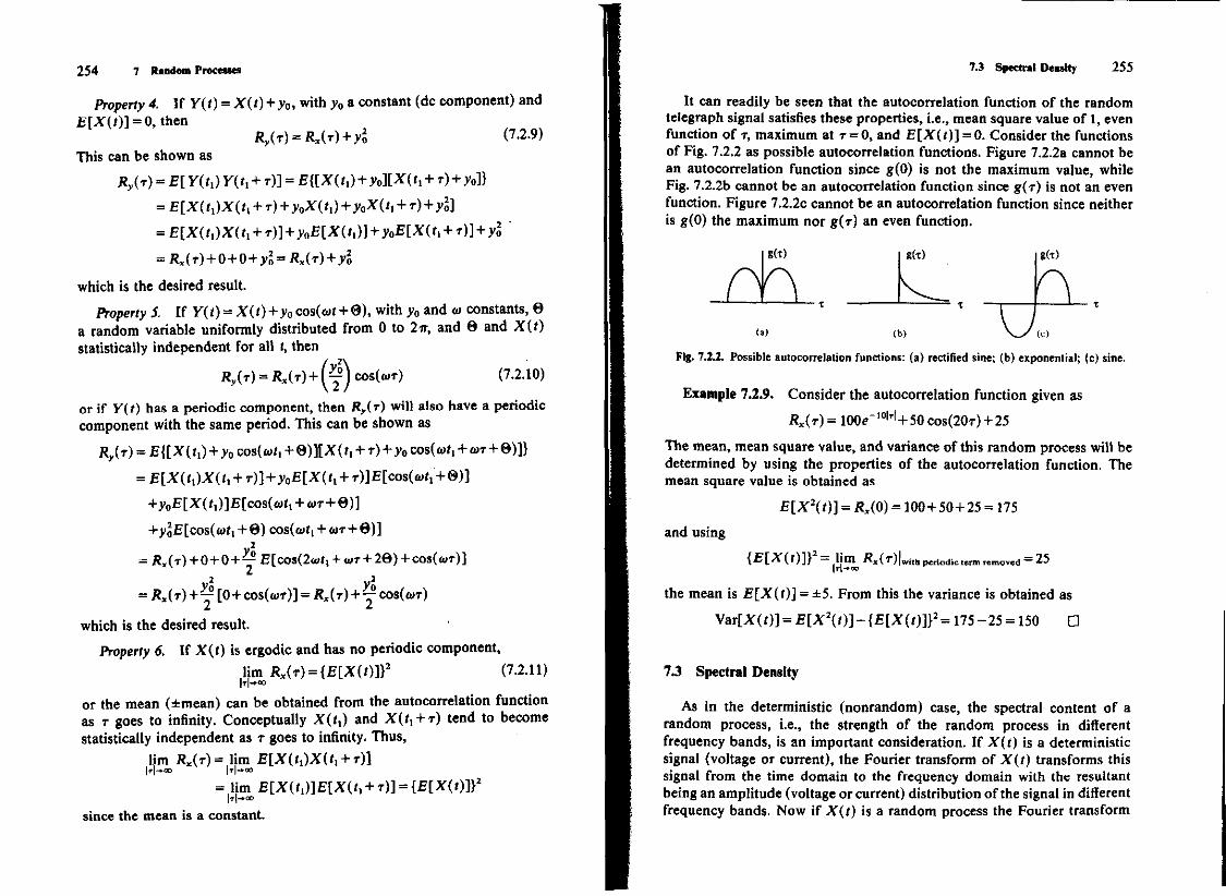
I t can readily be seen that the autocorrelation function of the random telegraph signal satisfies these properties, i.e., mean square value of 1, even function o f T, maximum at T = 0, and E [ X ( * ) ] = 0. Consider the functions of Fig. 7.2.2 as possible autocorrelation functions. Figure 7.2.2a cannot be an autocorrelation function since g(0) is not the maximum value, while Fig. 7.2.2b cannot be an autocorrelation function since g(r) is not an even function. Figure 7.2.2c cannot be an autocorrelation function since neither is g(0) the maximum nor g(r) an even function.
Example 7.2.9. Consider the autocorrelation function given as
K * ( T ) = 100e" , 0 | T , +50 cos(20r) + 25
The mean, mean square value, and variance of this random process wil l be determined by using the properties of the autocorrelation function. The mean square value is obtained as
E [ X 2 ( 0 J = RM = 100+50+25 = 175
and using
{E[X(t)]}2= l im ^ * ( r ) | w i l h p e r i o d ^ t e r m r e m o v e d = 25
|rl-»ac
the mean is E [ X ( f ) ] - ± 5 . From this the variance is obtained as
Var [X (0 ] = E [ X 2 ( 0 3 * { £ [ X ( ( ) ] } 2 = 175-25 = 150 •
7.3 Spectral Density
As in the deterministic (nonrandom) case, the spectral content of a random process, i.e., the strength o f the random process in different frequency bands, is an important consideration. I f X(t) is a deterministic signal (voltage or current), the Fourier transform of X(t) transforms this signal from the time domain to the frequency domain with the resultant being an amplitude (voltage or current) distribution of the signal in different frequency bands. Now i f X ( r ) is a random process the Fourier transform
256 7 Random Processes
of X(t) transforms this into the frequency domain, but since the random process is a function of both time and the underlying random phenomena, the Fourier transform is a random process in terms of frequency (instead of time). This transform may not exist and even i f i t does a random process does not yield the desired spectral analysis.
A quantity that does yield the desired spectral analysis is the Fourier transform (taken with respect to the variable T, time difference, of the function) o f the autocorrelation function of stationary (at least wide sense stationary) random processes. This Fourier transform is commonly called the power spectral density of X{t) and denoted SK(f) [ i t may also be written as Sx(a) where w = 2nf]. Thus, Sx(f) is given as
Sx(f)= P Rx(r) e~J2'fr dr (7.3.1a)
with the inverse Fourier transform given by
Sx(f) eJ2irfr df (7.3.1b)
Evaluating Eq. (7.3.1b) at T = 0 gives
Sx(f)df=E[X2{t)] (7.3.2)
K*(r) = j "
* x ( 0 ) = [ J -a
which justifies the name of power spectral density, since the integral over frequency yields a power (mean square value). The power spectral density then describes the amount of power in the random process in different frequency bands. [More precisely, it describes the amount of power which would be dissipated in a 1-0 resistor by either a voltage or current random process equal to X(t).] I f X(t) is an ergodic random process Eq. (7.3.2) can be written as
J>a> (7.3.3)
which is equivalent to the definition of total average power (which would be dissipated in a 1-H resistor by a voltage or current waveform).
For X(t) an ergodic random process an alternative form of the spectral density is
T-*oo 2T where
Fx(f) = j " T X(t) e~i2irf'dt (7.3.5)
7.3 Spectral Density 257
Example 7.3.1. Determine the power spectral density for the random telegraph signal of Fig. 7.1.3, where the autocorrelation function was determined in Example 7.2.8. The power spectral density is then determined as
Sx(f)= [" e ^ e ^ d r J —OO
0 Coo
ei2A-J2vf)T e - ( 2 A + / 2 i r / ) T ^
Jo
1 . 1 4A ^ 2\-j2wf 2 A + j 2 i r / ( 2 T T / ) 2 + 4 A '
Several properties o f power spectral densities wi l l now be given.
Property 1.
Sx(f)^0 (7.3.6)
That this is true can be observed by assuming that Sx(f)<0 for some frequency band. Then integrating only over this frequency band wil l yield a negative power, which is impossible, and thus Sx(f) must be nonnegative. This can also be observed from the alternative form of the spectral density, since it is an average of a positive quantity.
Property 2. Sx(-f) = Sx(f) (7.3.7)
or Sx(f) is an even function o f frequency. This can be shown by expressing the exponent o f Eq. (7.3.1a) as
e~J2irfr = cos(27r/T) - j sm{2nfr) to yield
Sx(f)= j Rx(T)[cos(2ir/T)-7sin(27r/T)]dT= f RX(T) COS(2IT/T) dr J-°° J_co
since Rx(T) is an even function of T, sin(2ir/r) is an odd function of T, the product RX(T) sin(2ir/r) is an odd function, and the integral of an odd function is 0. Finally, cos(2irfr) is an even function off, which makes Sx(f) an even function of /
Example 7.3.2. Determine E[X2(t)] and RX(T) for the random process X(t) with power spectral density Sx(f)-l/[(2ir/)2+0.04], -oo</<oo. Using Eq. (7.3.2) and J [ l / ( t > 2 + c 2 )] dv = (1/c) taxT^v/c)
^ • j ; ^ * - G ^ ) , ( S ) ' - i ® /=co
= 2.5
258 7 Random Processes
Since the power spectral density Sx{f) is o f the same form as the spectral density of Example 7.3.1, the autocorrelation function is of the form
Rx(T) = a e~fcW -oo < T < oo
The power spectral density, from Eq. (7.3.1a), is expressed as
Setting this equal to the given Sx{f) yields a = 2.5 and b = 0.2. Thus,
^ ( r ) = 2 . 5 e - ° - 2 W -oo<r<oo
a n d ^ ( 0 ) = 2.5 = E [ X 2 ( 0 ] . •
A noise random process is said to be white noise i f Us power spectral density is constant for all frequencies, i.e., i f
S « ( / ) = y - o o < / < c o (7.3.8)
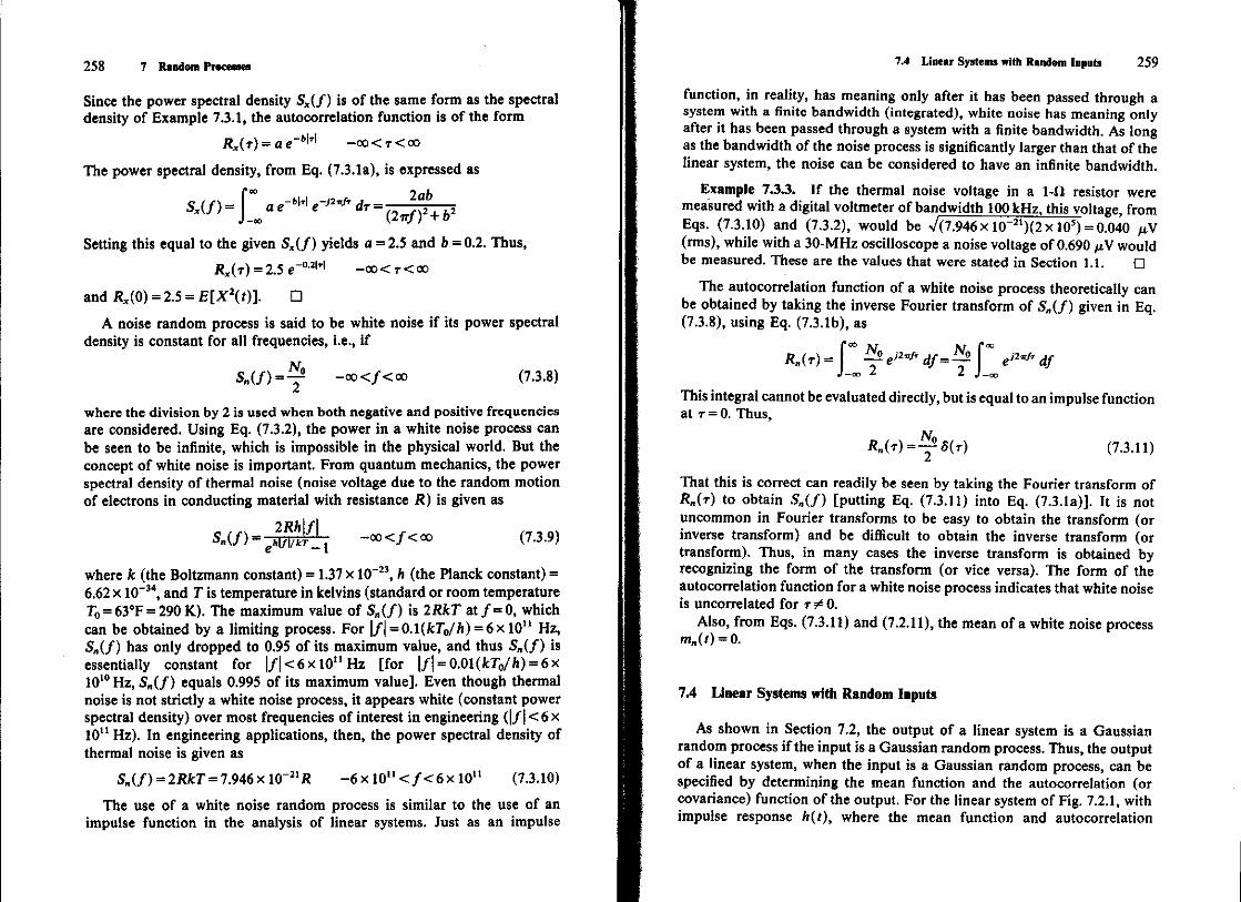
where the division by 2 is used when both negative and positive frequencies are considered. Using Eq. (7.3.2), the power in a white noise process can be seen to be infinite, which is impossible in the physical world. But the concept o f white noise is important. From quantum mechanics, the power spectral density of thermal noise (noise voltage due to the random motion of electrons in conducting material with resistance R ) is given as
where k (the Boltzmann constant) = 1.37 x 10" 2 3 , h (the Planck constant) = 6.62 x 10" 3 4 , and T is temperature in kelvins (standard or room temperature T 0 = 63°F = 290 K ) . The maximum value o f S „ ( / ) is 2RkT at f=*0, which can be obtained by a limiting process. For \f\ = Q.\(kT0/h) = 6x\Qil Hz, SH(f) has only dropped to 0.95 of its maximum value, and thus Sn(f) is essentially constant for | / | < 6 x l 0 M H z [for | / | = 0.01(k7o//i) = 6 x 10 1 0 Hz, Sn{f) equals 0.995 of its maximum value]. Even though thermal noise is not strictly a white noise process, it appears white (constant power spectral density) over most frequencies of interest in engineering ( | / | < 6 x 10" Hz). I n engineering applications, then, the power spectral density of thermal noise is given as
S„(f) = 2RkT = 7.946x l O " 2 1 * - 6 x 10" < / < 6 x 10" (7.3.10)
The use of a white noise random process is similar to the use of an impulse function in the analysis of linear systems. Just as an impulse
7.4 Linear Systems with Random Inputs 259
function, in reality, has meaning only after it has been passed through a system with a finite bandwidth (integrated), white noise has meaning only after it has been passed through a system with a finite bandwidth. As long as the bandwidth of the noise process is significantly larger than that of the linear system, the noise can be considered to have an infinite bandwidth.
Example 7.33. I f the thermal noise voltage in a 1-11 resistor were measured with a digital voltmeter of bandwidth 100 kHz, this voltage, from Eqs. (7.3.10) and (7.3.2), would be 7(7.946 x 10" 2 1)(2 x 10 s) = 0.040 / tV (rms), while with a 30-MHz oscilloscope a noise voltage of 0.690 would be measured. These are the values that were stated in Section 1.1. •
The autocorrelation function of a white noise process theoretically can be obtained by taking the inverse Fourier transform of S„(f) given in Eq. (7.3.8), using Eq. (7.3.1b), as
* » ( r ) = f ^ e ^ d f = ^ e^df J -co 2. 2 J -cc.
This integral cannot be evaluated directly, but is equal to an impulse function at T = 0. Thus,
K(r)=^S{r) (7.3.11)
That this is correct can readily be seen by taking the Fourier transform of R„(T) to obtain S„(f) [putting Eq. (7.3.11) into Eq. (7.3.1a)]. I t is not uncommon in Fourier transforms to be easy to obtain the transform (or inverse transform) and be difficult to obtain the inverse transform (or transform). Thus, in many cases the inverse transform is obtained by recognizing the form of the transform (or vice versa). The form of the autocorrelation function for a white noise process indicates that white noise is uncorrelated for T / 0.
Also, from Eqs. (7.3.11) and (7.2.11), the mean of a white noise process m„(0 = 0.
7.4 Linear Systems with Random Inputs
As shown in Section 7.2, the output of a linear system is a Gaussian random process i f the input is a Gaussian random process. Thus, the output of a linear system, when the input is a Gaussian random process, can be specified by determining the mean function and the autocorrelation (or covariance) function of the output. For the linear system of Fig. 7.2.1, with impulse response h(t), where the mean function and autocorrelation
260 7 Random Processes
function o f the input random process, are mx(t) and Rx(tttt2) respectively, the mean function of the output is obtained as
m,
or
,(r) = £ [ y ( t ) ] = - E [ j ° ° * - ( « ) / ! ( ( - « ) d u j = j E[X(u)]h(t-u)du
f oo Too mx(u)h(t-u) du = mx(t-u)h(u) du (7.4.1)
- 0 0 J - 0 0
Likewise, the autocorrelation function o f the output is obtained as
= E[j X ( ( , - u ) / i ( u ) d u | X ( i 2 - w ) A ( « ) r f w j
= £[I 1 X( f , -u )X( t 2 - iOM«)*( t>)<*u<*i>]
£ [ X ( ( , - u ) X ( t 2 - v)]h(u)h(v) du dv - 0 0 J - 0
The relationships of Eqs. (7.4.1) and (7.4.2) involving the mean function and the autocorrelation function are valid for any random process that is the output of a linear system. They have special meaning, however, in the case of a Gaussian random process, since a knowledge of these functions is sufficient to specify the random process.
For the special case of X( t) being wide sense stationary, mx( t) = mx and R-xOi, h) = K * ( T ) , where r - r 2 - r,. I n this case, the mean function of Y( (), Eq. (7.4.1), reduces to
• r J -a
my{t) = j mxh(u)du
or
my(t) = mx j h(u)du~my (7.4.3)
which is a constant. Also, the autocorrelation function of V ( r ) , Eq. (7.4.2),
7.4 Linear Systems with Random Inputs 261
reduces to
Ry(tx*h)= K(h-v-(tx-u))h(u)h(v)dudv J -OO J -OO
o r (7.4.4) poo r 00
K , ( T ) = Rx(r~v + u)h(u)h(v)dudv J —OO J —00
Thus, Y(t) is wide sense stationary i f X(t) is wide sense stationary. The power spectral density of the output of the linear system can be
obtained by rewriting Eq. (7.4.4) as j * co r<x> r co
Recognizing the integral with respect to v as H{f) and the integral with respect to u as H*(f) [ i f h(t) is a real function], this reduces to
Ry(r) = I Sx(f)\H(f)\2 eJ2"fT df= [°° Sy(f) eJ2"fr df
J -OO J - o o
Setting the integrands equal, since Fourier transforms are unique, yields
Sy{f) = Sx(f)\H(f)\2 (7.4.5) Example 7.4.1. Consider a white noise process, X(t), as an input to an
ideal low-pass filter, whose transfer function is shown in Fig. 7.4.1. With
and
/ M r ) = ^ 5 ( r )
S*(/) = y -oo</<oo
H(f)
1
- w o w
Fig. 7.4.1. Ideal tow-pass filter.
262 7 Random Processes
the output power spectral density, from Eq. (7.4.5), is obtained as
No -W<f< W
- O O < T < O 0 •
and the output autocorrelation function, from Eq. (7.3.1b), as
From the output autocorrelation for the ideal low-pass filter it can be seen that this filter has correlated the noise process. The mean square value or power in the output process is given as Ry(0) - t V N 0 , which is finite as expected.
Example 7.4.2. Consider the RC low-pass filter shown in Fig. 7.4.2. Again, the input is a white noise process with power spectral density N 0 / 2 .
R
X(i) V(t)
Fig. 7.4.2. RC low-pass filter.
The transfer function of this filter can be obtained, using a voltage divider (ratio of the impedance of the capacitor to the sum of the impedances of the resistor and the capacitor), as
or letting fe = l/{2wRC)
1 \/{)2irfC) R + l/ijlirfC) \+j2irfRC
H ( / ) = 1
- O O < / < 00 l+Jf/fc
The impulse response of this filter can be shown to be
h{t) = 2nfce-2°f<' ( i=0
= o otherwise
H(f) could also have been obtained by taking the Fourier transform of
7.4 Linear Systems with Random Inputs 263
h(t). The output power spectral density is obtained as
Sy(f) = SAf)\H(f)\2 = N0/2
1 -co < f < CO
and the autocorrelation function expressed as
which can be recognized as (or using a Fourier transform table, not evaluating the integral)
Ry{T)=Mike-2^\ _ Q 0 < T < 0 0
The RC low-pass filter correlates the noise process, and the mean square value of the output process is given as Ry(0) = 2irfcN0/4. •
As a final item consider a random process as the input to two linear systems as shown in Fig. 7.4.3. I f the input random process X{t) is Gaussian,
X(t)
h y(t) Y(i)
z<0
Fig. 7.4.3. Linear systems with common input.
then Y(t) and Z(t) are jointly Gaussian random processes. The cross-correlation of two random processes is defined in a manner similar to the autocorrelation. The cross-correlation of Y(t) and Z(t) is given as
RyAty,t2) = E[Y{tx)Z{t2)} (7.4.6)
For the Y(t) and Z ( f ) given in Fig. 7.4.3 the cross-correlation function is given as
RyAh ,t2) = E X(U - u)hAu) du | X(t2~ v)hAv) dvj
which can be expressed in terms of the autocorrelation function of the input as
When the cross-correlation function R y i ( r ) is a function only o f T and E[ Y{t)] and E[Z(t)] are constants, V( r ) and Z{t) are defined to be jointly wide sense stationary.
The cross-spectral density ( i f it exists) is defined as the Fourier transform of the cross-correlation function and written as
Syz(f)=r RyMe-i2"fTdT (7.4.8a) J - 0 0
Likewise, the cross-correlation function is the inverse Fourier transform of the cross-spectral density and given as
RyM=\ Syz{f)e}2^df (7.4.8b)
The cross-spectral density of Y(t) and Z ( r ) can be obtained by putting Eq. (7.3.1b) into Eq. (7.4.7b), which yields
RyAr)= P T IT Sx(f)ej2^~v+uUf\hy(u)hz{v)dudv J —OO J —OS L J —oo J
and interchanging the order of integration
RyM=11sAf) [IIky(u) e**fu
rf"][fLhM e~i2w/v d v ] d f
Recognizing the integral with respect to v as Hz(f) and the integral with respect to u as H*(f) [ i f hy(t) is a real function], this reduces to
RyM= P Sx(f)H*(f)Hz(f)eJ2^df= r Sy,(f)eJ2«*df J -oo J -oo
Setting the integrands equal yields
Syz(f) = Sx(f)Hf(f)H2(f) (7.4.9)
I f Hy(f) and Hz{f) are nonoverlapping, / ^ ( T ) = 0 for all T. I n addition, either Hy(f) or H r ( / ) must have zero response to a constant (dc) input; i.e., i f Hy(f) has zero response to a constant, Y(t) = 0 i f X"(f) = c. Since
Y(t) = X ( ! - u ) W " J - 0 0
Problems 265
this zero response to a constant implies
| hy{u)du=0 J— 00
and using this in Eq. ( 7 . 4 . 3 ) yields my(t) = 0. Thus, the covariance between Y(t) and Z{i) is zero, and i f X{t) is a Gaussian random process, Y(t) and Z(t) are statistically independent.
The covariance (or cross-covariance) function of the random processes Y(t) and Z{t) is defined, similar to Eq. (7.2.2), as
and the second property follows from Eq. (4.6.1) with X and Y replaced by Y(t) and Z(t), respectively.
In a manner similar to the definition of the time autocorrelation function given in Eq. (7.2.5), i f the random processes Y(t) and Z(t) are ergodic, then the time cross-correlation function of Y(t) and Z{t) is defined as
RYZ(T)= l im ~ [ Y(t)Z(t + r)dr (7.4.12)
Thus, when Y(t) and Z{t) are jointly ergodic random processes, the cross-correlation function of Y(t) and Z{t) can be obtained as a time average.
P R O B L E M S
' ' [7J . l . N For the random process X(t) = Acos(a)0t)+B$in(a)0t), where w 0 is a constant and A and B are uncorrected zero mean random variables having different density functions but the same variance o-2, determine whether X(t) is wide sense stationary.
\J.2.2.>or the random process X(t) = Ycos(2irl) and fY(y)={, -l^y^l, evaluate E[X(t)] and E[X2(t)] and determine whether X(t) is strict sense stationary, wide sense stationary, or neither.
7.2.4. Determine the covariance matrix o f the Gaussian random vector X T = (XUt)tX(t2), X(h)) when /, = 1, t2 = i.S, and fj = 2.25, where X(t) is a stationary Gaussian random process with mx(t) = 0 and R X ( T ) = s i n ( w T ) / ( i r T ) .
7.2.5. For a random process X(t) with autocorrelation function Rx(r) as shown in Fig. P7,2.5a, determine the autocorrelation function RV(T) for the system shown in Fig. F7.2.Sb[Y(t)~X(t) + X(t-3)].
- 2 - 1 0 1 2
Fig. P7.2.5..
X(t)
T=3 second delay
Ftg. P7,2.5b.
7.2.6. For a random process X(t) with autocorrelation function Rx(T) as shown in Fig. P7.2.5a, determine the autocorrelation function Ry(r) for the system with Y(t) = X(t-2) + X(t-5).
7.2.7. Determine E[X(t)], E[X2(0l and V a r [ X ( f ) ] for Rx(T) = 5 0 + COS(5T) + 10.
7.2.8. For Rx(T) as shown in Fig. P7.2.8, determine £ [ * ( ( ) ] » E[X2(t)], and V a r [ X ( t ) ] .
Ftg. P7.2.8.
Problems 267
7.2.9. For RX(T) as shown in Fig. P7.2.9, determine E[X(t)], E[X2(t')], and V a r [ X ( / ) ] .
R x ( t )
> \ \
i •
Fig. P7.2.9.
7.2.10. Show that the mean function mx(i) = 0 and the autocorrelation function Rx(T) = (1~\T\/T), - T = = T < T, for the binary random process X(t) = A„ i T + u < t < ( i + 1) T + v, -co < i < co, where V i s a uniform random variable with fv( v) = 1/ T, Os u < T, J>(A, = 1) = P(At = - 1 ) = 0.5, and {A,} and V are statistically independent.
7.2.11. For the periodic function X(t) = . . . t - I , + 1 , + 1 , - 1 , + 1 , - l , - 1 , . . . where each ±1 is on for 1 sec and T = 7sec, determine the time autocorrelation function Rx(r) (obtain for T = 0, 1,2.3,4,5,6).
7.2.12. For the periodic function X(t) = . . . , - 1 , + 1 , + 1 , + 1 , - 1 , + 1 , . . . where each ±1 is on for 1 sec and 7" = 6 sec, determine the time autocorrelation function RX(T) (obtain for T = 0 , 1 , 2, 3, 4, 5).
7.3.1. Determine the power spectral density Sx(f) for RX(T) = 1, - 2 s r s 2 .
7.3.2. Determine the power spectral density for the binary random process o f Problem 7.2.10 with T= 1.
7.3.3. Determine E [ X ( r ) 3 , E[X2(t)], and R T ( T ) for the random process X(t) with power spectral density S,(J) = IO/[(27r/) 2 + 0.16], - c o < / < c o .
7.3.4. ForS , ( / )asshowninFig . P7.3.4,determine £ [ * ( ( ) ] , E[X" 2 ( f ) ] ,and K x ( T ) .
2
Sx(0
0 5
Fig. P7.3.4.
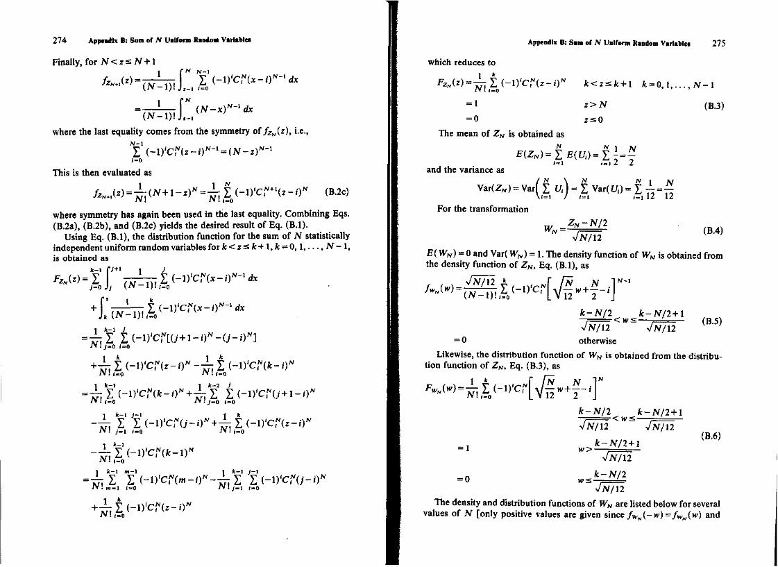
7.3.5. For Sx (f) as shown in Fig. P7.3.5, determine E[X( / )], E[X2(t)l and RX (r).
7.3.6. Determine the thermal noise voltage in a resistor when it is measured with a 1-MHz oscilloscope and when it is measured with a 5-MHz oscilloscope.
268 7 Random Processes
Sx(0
3
f -4 0
Fig. P7J.5.
73.7. Determine the thermal noise voltage in a 1-ft resistor when it is measured with (a) a 10-MHz oscilloscope and (b) a 50-MHz oscilloscope.
7.3.8. Can g ( / H 5 cos(2ir/) be a power spectral density for the wide sense stationary random process X(t)l
7.4.1. Determine the output power spectral density and the output autocorrelation function for a system with impulse response h(t) - e~', t aO, whose input is a white noise process X(t) with spectral density Sx(f) = N0/2, -ao</<oo.
7.4.2. Determine the output power spectral density and the output autocorrelation function for a system with impulse response h(t) = t.Oss ts I , whose input is a white noise process X(t) with spectra density Sx(f)= NJ2, -oo</<oo.
7.4J. Determine the cross-correlation function of Z,(() = X{t) + Y(t) and Z2{t) = X(t)-Y(t)t where X(t) and V(t) are statistically independent random processes with zero means and autocorrelation functions Rx(T) = e~M, -oo< r<oo, and i?,,(T) = 2e" | T |, -OO<T<OO.
7.4.4. For the random processes X ( i ) = A cos {t»0t) + B sin(w 00 and Y(t) = Bcos(w 0 0-Asim> 0 <) where w 0 is a constant and A and B are uncorrected zero-mean random variables having different density functions but the same variance <r2, show that X(t) and Y(t) are jointly wide sense stationary.
7 A S . For the two periodic functions X(t) = . . . , - 1 , +1, +1 , - 1 , +1 , - 1 , - 1 , . . . and Y(t) = ..., - 1 , +1, +1 , - 1 , - 1 , - 1 , + 1 , . . . where each ±1 is on for 1 sec and T = 7sec, determine the time cross-correlation function RXY{T) (obtain for T = 0,1,2,3,4,5,6).
Appendix A Evaluation of Gaussian Probabilities
A.1 Q Function Evaluation
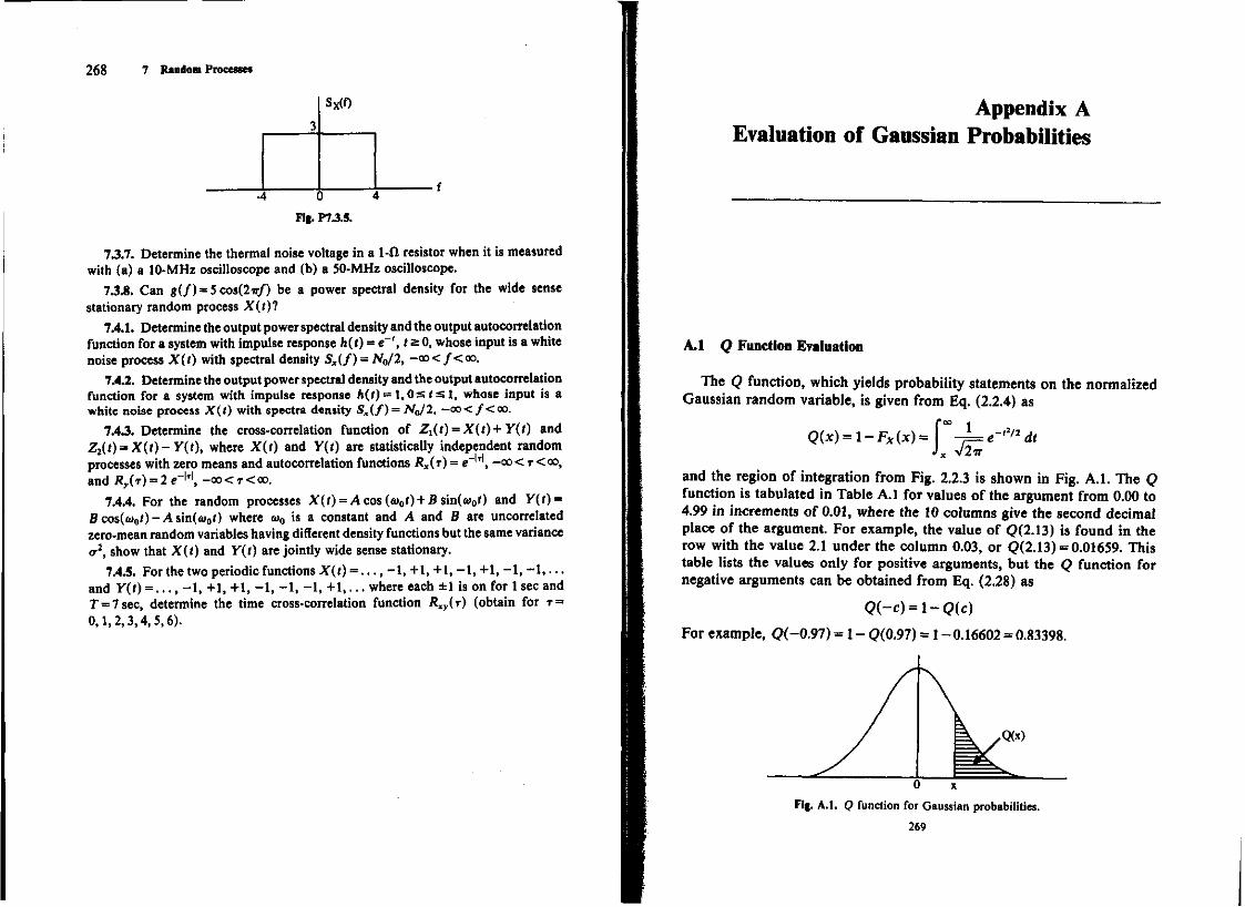
The Q function, which yields probability statements on the normalized Gaussian random variable, is given from Eq. (2.2.4) as
<?(*) = 1 - F x ( x ) = [ " J x V2ir
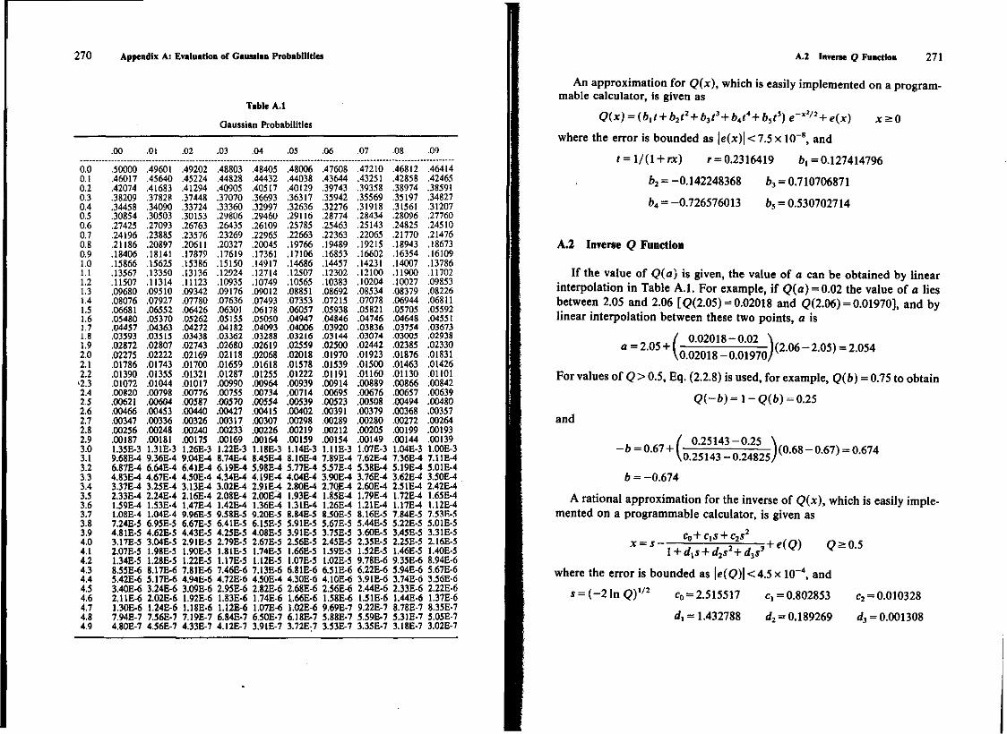
and the region of integration from Fig. 2.2.3 is shown in Fig. A .1 . The Q function is tabulated in Table A.1 for values o f the argument from 0.00 to 4,99 in increments o f 0.01, where the 10 columns give the second decimal place of the argument. For example, the value o f <?(2.13) is found in the row with the value 2.1 under the column 0.03, or <?(2.13) = 0.01659. This table lists the values only for positive arguments, but the Q function for negative arguments can be obtained from Eq. (2.28) as
C?(-c) = l - Q ( c )
For example, Q(-0$7) = 1 - <?(0.97) = I - 0.16602 = 0.83398.
0 x Fig. A.1. Q function for Gaussian probabilities.
269
270 Appendix A: Evaluation of Gaussian Probabilities
where the error is bounded as \e(x)\ < 7.5 x 10" 8, and
* = 1/(1 + rx) r = 0.2316419 bx = 0.127414796
b2 = -0.142248368 6 3 = 0.710706871
6 4 = -0.726576013 bs = 0.530702714
A.2 Inverse Q Function
If the value of Q(a) is given, the value of a can be obtained by linear interpolation in Table A .1 . For example, i f Q(a) = 0.02 the value of a lies between 2.05 and 2.06 [Q(2.05) = 0.02018 and <?(2.06) = 0.01970], and by linear interpolation between these two points, a is
/ 0.02018-0.02 V a = 2.05 + ( (2.06 - 2.05) = 2 054
\0.02018-0.01970/V '
For values of Q > 0.5, Eq. (2.2.8) is used, for example, Q(b) = 0.75 to obtain
The density function and the distribution function for the sum of N statistically independent random variables uniformly distributed from 0 to 1 is derived. The results are piece wise continuous functions with different expressions over each unity interval. For ZN the sum of these uniform random variables, a normalized version o f the sum, WNt is defined where the mean of WN is 0 and the variance of WN is 1. The density function and distribution function for WN are also developed. The density function of this normalized sum then facilitates a direct comparison with the normalized Gaussian density function.
Letting ZN be the sum of N statistically independent uniform random variables as
Z i = t / i
ZN = ZN.{+UN N = 2 , 3 , . . .
where
fUl{u,) = l 0<u,*l 1 - 1 , 2 , . . .
= 0 otherwise
the density function of the sum of N statistically uniform random variables is given as
^ > > = 7 ^ T T ^ £ ( - D ' C f U - O 1 * - 1 k<z*k + \
(IS - 1 ) 1 i-o
fc = 0 , l , . . . , N - l (B.1)
= 0 otherwise 272
Appendix B: Sum of N Uniform Random Variables 273
This will be proved by using mathematical induction. Before starting, note from symmetry that
fz„(2)=fzN(N-z) N=l,2,...
and the density function of ZN+t is obtained from the density function of ZN and the density function of UN+i by convolution as
/ z N + 1 ( z ) = fvN+,{z-x)fZN{x) dx J -co
For a starting value, N = 1
/z ,(«) = l 0 < r = s l
and Eq. (B . l ) holds. Now assume Eq. (B . l ) is true for N and show that it is true for N+l. Three ranges wil l be considered separately.
First, for 0 < z < l
Now, for fc<z<;Jfc+l, it = 1,2, . . . , N-l,
+ri(- i ) 'cf(x- i) w - , rfxi Jk *-Q J
+ J \ - i ) i c f ( x - . r - i J x ]
= ^ [ | V i > ' c r { ^
= ^ [ ^ + | / - i ) f c c r ( z - k ) w - | ] ( - i r l c ^ 1 ( 2 - ; ) w j
Using the relationship C ? + C,1 , = C?+l yields
faJti-jfiii-lYcr^z-i)" (B.2b)
274 Appendix B: Sum of TV Uniform Random Variables
Finally, for N < z ^ N +1
where the last equality comes from the symmetry of fz„(z), i.e.,
1-0 This is then evaluated as
/ z N + l U ) = ~ ( N + l - z ) ^ = ^ | o ( - l ) ' c r i ( z - , r (B.2c)
where symmetry has again been used in the last equality. Combining Eqs. (B.2a), (B.2b), and (B.2c) yields the desired result of Eq. (B . l ) .
Using Eq. ( B . l ) , the distribution function for the sum of N statistically independent uniform random variables f o r f c < z ^ f c + l , f c - 0 , 1 , . . . , N - 1 , is obtained as
F - ( z ) = i r ( r a . t M ) ' c r ( x - ' r , d x
= ^ r I £ ( - i ) , c f [ ( y + i - o K - 0 - O w ] TV! j -o (=o
i ( - D ' c r t r - o " ~ i ( - D ' c ^ t - . r Pi ! i - o J V I f - o
- 1 5 7 1 ( - D ' C , N ( * - 0 N + ^ " f I ( - D ' c f o + i - o 1 *
i 'li-iycru-ir+^-.i(-i)'c,"(z-oN
JV! ; _ 1 /-o JVi (=0
~ Z ( - l ) ' C , w ( i k - l ) " iV I 1=0
4 l I ' t - D ' c r t m - . T - T j : ! ' I ( - i ) ' c f O - O "
Appendix B: Sum of Uniform Random Variable* 275
which reduces to
FZn(Z) = ~ i(~l)'C?(z-i)N k<z^k+l fc = 0 , l , . . . , N - l
= 1 2>N (B.3)
= 0 z^O The mean of ZN is obtained as
i - i ; - i 2 2 and the variance as
( N \ N N 1 XT
I t / , = 1 V a r ( U , ) = L - U - £ i=i / < = i (=i 12 12
For the transformation „ , ZN - N/2
E( WN) = 0 and Var( W N ) = 1. The density function of WN is obtained from the density function o f Z N , Eq. (B . l ) , as
k-N 2 k-N/2 + \ ,——- < w < — ' — (B.5)
JN/U V N / 1 2 v ' — 0 otherwise
Likewise, the distribution function of WN is obtained from the distribution function of ZN, Eq. (B.3), as
k-N/2 k~N/2 + l
VAT/12 V J V / 1 2 (B.6)
- 1 k-N/2 + 1 - 1 w > — V N / 1 2
_ n k-N/2
V N / 1 2
The density and distribution functions of WN are listed below for several values of N [only positive values are given since fwN{-w) = fwN{w) and
276 Appendix B: Sum of N Uniform Random Variables
f v N ( - H > ) = 1 - F W N ( W ) ] . For each N and each range the density function is given first and one minus the distribution function is given next
N=\ A = B = 0.2887 C = l
0 < w s 1.732 B C ( l / 2 - A w )
N = 2 A = B = 0.4082 C = 0.5
0 < w < 2 . 4 4 9 B(\-Aw) C ( l - A w ) 2
N = 4 A = 0.5774 B = 0.09623 C « 0.04167
1.732 < w ̂ 3.464 B[(2 - A w ) 3 ] C [ ( 2 - A w ) 4 ]
0 < w < 1.732 B[(2 - Aw)3 - 4 ( 1 - Aw)3] C [ ( 2 - A w ) 4 - 4 ( 1 - A w ) 4 ]
N = 8 A = 0.8165 B = 0.0001620 C = 2.480 x 10~5
3.674 < w ̂ . 4.899 B[(4 - A H > ) 7 ] C [ ( 4 - A w ) 8 ]
2.449 < w £ 3.647 B[(4 - Aw)7 - 8(3 - Aw)7] C [ ( 4 - A w ) 8 - 8 ( 3 - A w ) 8 ]
1.225 < w < 2.449 B [ ( 4 - A w ) 7 - 8 ( 3 - A w ) 7 + 28(2 - A w ) 7 ] C [ ( 4 - A w ) 8 - 8 ( 3 - A w ) 8 + 2 8 ( 2 - A w ) 8 ]
0 < w < 1.225 B [ ( 4 - A w ) 7 - 8 ( 3 - A w ) 7 + 2 8 ( 2 - A w ) 7 - 5 6 ( l - A w ) 7 ] C [ ( 4 - A w ) 8 - 8 ( 3 - A w ) 8 + 2 8 ( 2 - A w ) 8 - 5 6 ( l - A w ) B ]
JV=12 A = l B = 2.505 x l O " 8 C = 2.088 X 10~9
5 < w ^ 6 B [ ( 6 - w ) n ] C [ ( 6 - w ) 1 2 ]
4 < w < 5 B [ ( 6 - w ) n - 1 2 ( 5 - w ) u ] C [ ( 6 - w ) , 2 - 1 2 ( 5 - w ) 1 2 ]
3 < w s 4 B [ ( 6 - w ) 1 1 - 1 2 ( 5 - w ) , 1 + 6 6 ( 4 - w ) n ] C [ ( 6 - w ) , 2 - 1 2 ( 5 - w ) 1 2 + 6 6 ( 4 - w ) 1 2 ]
2 < w s 3 B [ ( 6 - w ) u - 1 2 ( 5 - w ) 1 , + 6 6 ( 4 - w ) 1 1 - 2 2 0 ( 3 - w ) 1 1 ] C [ ( 6 - w ) I 2 - 1 2 ( 5 - w ) 1 2 + 6 6 ( 4 - w ) l 2 - 2 2 0 ( 3 - w ) 1 2 ]
K w s 2 B [ ( 6 - w ) n - 1 2 ( 5 - w ) n + 6 6 ( 4 - w ) n - 2 2 0 ( 3 ~ w ) n
+ 4 9 5 ( 2 - w ) 1 1 ] C [ ( 6 - w ) , 2 - 1 2 ( 5 - w ) , 2 + 6 6 ( 4 - w ) 1 2 - 2 2 0 ( 3 ^ w ) 1 2
+ 4 9 5 ( 2 - w ) 1 2 ] 0 < w = s l B [ ( 6 - w ) 1 1 - 1 2 ( 5 - w ) I , + 6 6 ( 4 - w ) 1 1 - 2 2 0 ( 3 - w ) n
+ 4 9 5 ( 2 - w ) n - 7 9 2 ( l - w ) M
C [ ( 6 - w ) 1 2 - 1 2 ( 5 - w ) l 2 + 6 6 ( 4 - w) 1 2 -220(3 - w)12
+ 4 9 5 ( 2 - w ) l 2 - 7 9 2 ( l - w ) 1 2
Appendix B: Sum of JV Uniform Random Variables 277
f w N < w )
Fig. B . l . Density function for the sum of JV uniform random variables.
Figure B . l gives a comparison of the density function of the normalized Gaussian random variable with the density function of WN for N = l , 2, 4, 8. From this figure it can be seen that the density functions are very close for N as small as 8. Likewise, for one minus the distribution function (the Q function) with w = 1 (1 standard deviation) the error relative to the Gaussian probability for N = 4, 8, and 12 is 4.2, 2.0 and 1.3%, respectively, which is quite close. Even for w = 2 (2 standard deviations) the error is small; i.e., for N = 4, 8, and 12 the error is 6.5, 3.2, and 2 .1%, respectively. But for w = 3 (3 standard deviations) the error relative to the Gaussian probability for N = 4,8, and 12 is 84.1,38.8, and 25.4%, respectively, which is quite large. Also, for w = 4 (4 standard deviations) the error for N - 4, 8, and 12 the error is 100, 93.4, and 73.1%. I t can be concluded that the sum of uniform random variables for small N is a good approximation to a Gaussian random variable i f the argument of the variable is within 2 standard deviations, but is a poor approximation for values on the tails (large arguments) of the random variable.
Appendix C Moments of Random Variables
The mean (first moment), the variance (second central moment), and the characteristic function (Fourier transform of the density function or probability function) are given for some frequently encountered random variables. Along with these moments, the range where the probability density function or probability function is nonzero is given and the range of the parameters o f the probability density function or probability function is given.
Table C . l gives these moments for the discrete random variables along with their probability function. Table C.2 gives these moments for the continuous random variables along with their probability density function.
Table C.1
Moments Tor Discrete Random Variables
Bernoulli P(X = fc) = p k ( l - p ) l _ k fc = 0 , l 0 < p < l E(X)=p V a r ( X ) - p ( l - p ) * x ( « ) - p c > , + l - p
Binomial P(X = k)=C%pk(l-p)N-k fc = 0 , l , . . . , N JV-1 ,2 ,3 , . . . 0 < p < l E(X) = Np Var(X) - JVp{l - p ) 4>x(<»)« [p +1 ~p]N
Poisson e~aak
P(X = k) = —— ft-0,1,2,... 0 < d « » Jfc!
E(X) = a Var(X) = a 4>x(<o) = exp[a (exp<» -1)]
Geometric
P(X = k) = (l-p)k-1p fc=l,2,3,... 0 < p < t
B W - i V a r ( X » = i ^ M m ) m - l £ —
278
Appendix C: Moments of Random Variables 279
Table C.2
Moments for Continuous Random Variables
Uniform
fx(x)=-l— -<x><a<x<b«x> b-a b + a (b-a)2
e J ^ _ , j ^ E(X)= — Var(X) = ^ - p - 4>xM = ~
2 12 j(b-a)o>
Gaussian
r < ^ 1 r - ( * - ^ ) 2 i Jx(x) = —=:exp\ • -oo< x <oo -oo<u<oo 0<«r<oo
E{X) = n Var(A") = a2 <f>x{a>) = e x p O p - « V / 2 )
Exponential
fx{x) = a e-°* 0< x <oo 0< a <oo
E(X)=- Var(X) = \ <M<») = -a a 1-/6
Gamma
\ah+lxb~\ ^ ^ ^ L n f e + D j e "X 0 - * < 0 0 0<a<co 0< b<oo
E m = t ± l V a r W , < i ± i M m ) J , a a \ a)
Cauchy
/ x W = ( f ) ( ^ + ^ ) - ® < * < ° ° 0<a<oo
E(X) undefined Var(Jt)=;oo <px(w) = e~"M
Rayleigh
fx(*)m(^j e j t p ( ~ ^ ~ ) 0^x<co Q<b<eo
E{X) = 4vbJ2 Var(X) = t 4 ~ f f ) ! >
2
Beta
r (a + 6+2) /x (*) = , , , „ , . , , . * a ( t - * r O s x s l 0 s f l < o o 0^&<cc 1 (a +1 JI (o +1)
o + e + 2 (a + 6 + 3)(a + / i + 2)3
Appendix D Matrix Notation
An introduction to matrix notation and examples of matrix manipulation are given in this appendix. A matrix is an array of numbers or symbols and its utility is the ease of representing many scalar quantities in shorthand notation. Matrices wi l l be represented by boldface letters. The general matrix A is given as
flu an ' ' 0\m
A = <*22 • = {at})
<*»2 ' * anm
where there are n rows and m columns and A is referred to as an n x m matrix. The element in the ith row and jth column is atJ and the set representation means the set of all elements a„. I f n = m, A is said to be a square matrix. The transpose o f the matrix A, A T , is the matrix obtained by interchanging the rows and columns o f A and is written
A T - { f l j , }
and the element in the i th row and the j t h column is a,,. I f A is n x m, A T
is m x R.
Example D . l . For
A = 1 4 2 5 3 6
280
Appendix D: Matrix Notation 281
a 3 x 2 matrix, the transpose is
a 2 x 3 matrix. • A row vector is a matrix with a single row and a column vector is a
matrix with a single column. The vectors considered here wi l l normally be column vectors, which makes the transpose a row vector. For x an n x 1 column vector, the transpose
xr = {Xi} = [xltx2,...,x„]
is a 1 x n row vector. Two matrices are equal
A = B = { b y } = {a t f }
i f a,/ = bif for all i and j , which implies that A and B must be the same size. The matrix A is symmetric i f
A = A T = {a,,} = { a y }
or a y = ajt for all i and j . To be symmetric A must be a square o r n x n matrix. For matrix addition to be defined, the matrices of the sum must be of
the same size. I f A and B are both nxm matrices the matrix addition is defined as
C = A + B = {a t f + 6 t f} = {c,,}
where the sum matrix is also n x m . Thus, an element in C is the sum of the corresponding elements in A and B. I t can easily be shown that matrix addition is both associative and commutative.
Example D.2. I f A and B are given as
" l 4" "2 - f A = 2 5 B = 7 -3
3 6 8 1
then the sum of A and B is
C = 3 9
11 •
The product of a scalar d and an n x m matrix A is defined as
B = d A = {da,,} = {*>,,}
282 Appendix D: Matrix Notation
where B i s n x m and each element in the product is the scalar times each corresponding element in A.
Example D.3. For A given in Example D.2, the product of d = 3 and A is
" l 4" "3 12" B = 3 2 5 = = 6 15
3 6 9 •
18
The multiplication of the two matrices A n x m and B m x p is defined as
C = AB = | j [ aJfc6yJ = { c y }
where C is an n x p matrix. The yth element of the product matrix is obtained as a summation of the elements in the i th row of A (the matrix on the left in the product) times the elements in the jth column of B (the matrix on the right). For these terms to match up, the number of elements in the i th row of A must equal the number of elements in the jth column of B; i.e., the number of columns of A must equal the number of rows of B for the multiplication to be defined. Matrix multiplication may not be commutative,
A B / B A
since for A n x m and B m xp , the product BA (p / n) is not defined. Even i f the product BA was defined (A is n x m and Bis m x n) , matrix multiplication is in general not commutative.
which is obtained as the sum of the product of elements in the i th row times corresponding elements in the jth column. This product reduces to
Appendix D: Matrix Notation 283
For A n x m, B m x p, and C p x q
= K } { t 6 ^ } = A(BC)
and matrix multiplication is associative. The result of the product is an n X q matrix.
The transpose of the product of matrices is the product of the transposes of the matrices in reverse order, i.e.,
( A B ) T = aikbkJJ = ajkbki} = j % bkiaJk} = B T A T
I f A is n x m and B is m x p, AB is n x p and ( A B ) T is p x n. Likewise, B T
is p x m, A T is m x n, and B T A T is p x n. A bilinear form is given as
{" 1 f n n " I n n
I \{yt} = \ £ £ xkakryr \ = £ £ xkakryr
where x T is 1 x n, A is n x n, and y is n x 1, which makes the bilinear form a scalar. When y = x, this form is called a quadratic form or x T A x is a quadratic form (a scalar). A special case of the quadratic form is
x T x = 1 xl
which is the magnitude of the vector squared. I f A is an n x n (square) matrix and i f for a matrix B (n x n),
BA = AB = I
where I is the identity matrix, B is said to be the inverse of A (B = A - 1 ) . B and I are w x n matrices and I has l's on the main diagonal and O's everywhere else.
In order to evaluate the inverse of a matrix a few terms wi l l first be defined. Letting Mi} be the minor of the element ai}, Mi} is equal to the determinant formed by deleting the i th row and the yth column of A. Also, letting A y be the cofactor of the element atJ,
A t f = ( - l ) ' ^ M t f
The determinant of A is given in terms of the cofactors as n n
|A| = OyAfJ = I OyAtj
284 Appendix D; Matrix Notation
which states that the determinant can be obtained by summing the product of elements of any row times their corresponding cofactors or by summing the product of elements of any column times their corresponding cofactors. I f B equals A with the jth column replaced by the ith column (columns i and j are the same in B), the determinant of B is 0 and
n |B| = 0 = I a w 4 y i*j
fc-i
The determinant is also 0 i f the jth row is replaced by the i th row (rows i and j are the same). Combining these statements with |A[ yields
L a k , A v - £ a,kAjk = 8,j\X\ k-\ k-l
where Sv « 1 , i - a n d SfJ - 0, i Now Cof A = (Ay) , Cof A T = {A*}, and
A C o f A T = { t alkAJk} = { | A | 5 t f } = | A | l
i f |A| * o
A - l = Cof A T / | A |
Also, ( A B ) - , - B " , A - 1 and ( A " 1 ) T = ( A T ) - 1 .
Example D.5. Consider the matrix
A =
The cofactors are calculated as
1 2 3 - 1 4 - 2 -3 6 5
A „ =
A 2 i = -
4 - 2 6 5
2 3 6 5
2 3 4 - 2 ^ 3 1 =
which yields
= 32
= 8
= -16
A 2 2 =
-4 3 2 =
- 1 - 2 -3 5
= 11 A 1 3 = - 1 4 -3 6
1 3 -3 5
1 3 - 1 - 2
= 14 A „ = -
— 1 A 3 3 =
1 2 -3 6
1 2 - 1 4
= 6
= -12
= 6
Cof A = 32 11 6
8 14 -12 -16 - 1 6
Appendix D: Matrix Notation 285
Now
|A| = a 1 I A „ + a 1 2 A l 2 + a 1 3 A I 3 = l(32) + 2 ( l l ) + 3(6) = 72
and finally the inverse is
32 A " 1 - ^ 11
72
8 -16 14 - 1
6 -12 •
A n alternative procedure for finding a matrix inverse is the Gauss-Jordan method. This method consists of solving the matrix equation AB = I for B, which is A " 1 . By performing row operations the augmented matrix [ A : I ] is manipulated to the form [ I : B ] , which yields the inverse directly.
Example D.6. For A of Example D.5 the augmented matrix is given as
1 2 3 : 1 0 0 -1 4 - 2 : 0 1 0 -3 6 5 : 0 0 1
1 2 3 : 1 0 0 0 6 1 : 1 1 0 0 12 14 : 3 0 1
where in the first step the element in row 1 column 1 is normalized to 1 to obtain a new row 1. Next a new row 2 is obtained, such that the element in column 1 is 0, as old row 2 minus ( - 1 ) times new row 1, and a new row 3 is obtained, such that the element in column 1 is 0, as old row 3 minus (—3) times new row 1.
I n the second step the element in row 2 column 2 is normalized to obtain a new row 2. Then a new row 1 is obtained, such that the element in column 2 is 0, as old row 1 minus (2) times new row 2, and a new row 3 is obtained, such that the element in column 2 is 0, as old row 3 minus (12) times new row 2. The second and third steps are given as
"l 0 f : 2 3
1 o" "l 0 0 : 4 9
l 5
2" ~5
-* 0 1 i l '
l 6"
l 6 0 -* 0 1 0 : 11
72 7
36 l
-12 0 0 12 : 1 - 2 1 0 0 1 : 1
U 1
~6 l
12 _
As shown for the third step the element in row 3 column 3 is normalized to obtain a new row 3. Then a new row 1 is obtained, such that the element in column 3 is 0, as old row 1 minus ( |) times new row 3, and a new row 2 is obtained, such that the element in column 3 is 0, as old row 2 minus (I) times new row 3.
286 Appendix D: Matrix Notation
Thus A 1 is obtained as
A " ' =
« I _2 9 9 9 11 7 75 36 J _ 1 12 6
-ft ft which is the same result as in Example D.5. •
The rank r of an n x m matrix A is the size of the largest square submatrix of A whose determinant is nonzero. A symmetric n x n matrix A is positive definite i f the quadratic form x T A x > 0 for each nonzero x and is positive semidefinite i f the quadratic form x T A x s 0 for each nonzero x and x T A x = 0 for at Least one nonzero x. The rank of A is equal to n i f A is positive definite, and the rank o f A is less than n i f A is positive semidefinite. Also, a,i>0 for all 1 ,2 , . . . , n i f A is positive definite, and a „ £ 0 for all i = 1 ,2 , , . . , n i f A is positive semidefinite.
A matrix A is positive definite i f and only i f the leading principal minors are greater than zero, i.e.,
a M > 0 , a,, a12
<*2I <*22 > 0 A| > 0
Likewise, a matrix A is positive semidefinite i f and only i f the leading principal minors are greater than or equal to zero.
In Section 4.4 the quadratic form of the exponent of the N-dimensional Gaussian density function must be positive semidefinite and XZ1 or % x (an n x n ) is a positive semidefinite matrix. That this is so can be seen by observing that for any subset of the random variables the determinant of the covariance matrix o f the subset must be greater than or equal to zero. The subsets can be picked such that all of the leading principal minors are greater than or equal to zero, which makes Xx positive semidefinite. I f X , is positive definite (rank n), then there is no impulse function in the density function ( i f r a n k < n there would be an impulse function in the density function). For the transformation Y = A X + B where Xy=* KXXAT, Xy is at least a positive semidefinite matrix since it is a covariance matrix. I f A is m x n Xy is m x m and i f m > n the rank of A is at most n and the rank of Xy at most n or Xy cannot be positive definite (there must be an impulse in the density function of Y ) .
An n x n matrix A is positive definite i f and only i f there exists an n x n matrix B of rank n such that B T B = A. Likewise, a n n x n matrix A is positive semidefinite i f and only i f there exists an n x n matrix B of rank less than n such that B T B = A. This property is used in Section 5.6 to obtain a transformation from statistically independent random variables to random variables with a desired covariance matrix.
Appendix D: Matrix Notation 287
Example D.7. Consider the Gaussian random vector YT = (YU Y2, Y3) with n j = (0,0,0) and
16 12 20 12 13 11
20 11 29
Since
16 > 0 , 16 12 12 13
= 0 16 12 20
= 64>0 , and 12 13 11 20 11 29
the rank o f Xy is 2. Thus / v ( y ) contains an impulse function. The impulse function can be determined using Eq. (5.6.2) to obtain T (Y = TX with 2* = I ) as
4 0 3 2 5 - 2
where t3i = 0 (and the third column is omitted). Then using Eq. (5.6.4) A (X = AY) is obtained as
f 0.25 0"| L-0.375 0.5 J
where the last row of A is omitted since t33~0. Finally, 1 0'
Y = T A Y = 0 1
2 - 1
which yields the dependency Y3-2Yt- Y2. Letting Y ' T = ( K , , Y 2 )thecondi-tional density of Y3 given Y' is the impulse (obtained from Y3 = 2Y{~ Y2) given as
Now
and
/ v 3 | v ( y 3 | y ' ) = 5 ( y 3 - 2 y , + y 2 )
« - - [ z a
j _ r 13 - i 2 i 6 4 L - 1 2 16}
288 Appendix D: Matrix Notation
which gives
/v (y ' ) = ^ - c x p [ - ( 1 3 y l - 2 4 y 1 y 3 + l 6 y 5 ) / 1 2 8 ] l O T T
-oo<y!<oo, - o o < y 2 < ° °
The density function of Y is then obtained as
/ v ( y )= /v (y ' ) / v3 iv ( ^ ly ' )
or
/ v ( y ) = 7 T - e x p t - ( 1 3 v 1 - 2 4 y 1 y 2 + 16^)/128] 5 ( y 3 ~ 2 y , + v 2 ) ' • l o i r
Appendix E Mathematical Quantities
E.l Trigonometric Identities
e,x - cos x +j sin x sin x sin y =* J[cos(x-y)-cos{x + y)]
e1" + e~JX sin x cos y * K>i n(* +y)+sin(x - y)] cos x -
2
sin x = -V
cos(x ± y) = cos x cos y T sin x sin y
' ( X ± f ) = T 8 i
sin(x ± y) * sin x cos y ± cos x sin y
cos x + cos y = 2 cos[$(x + y)] cos[J(x - y)]
cos x-cos y = ~2 sin[|(x + y)] s in[ i (x-y) ]
sin x ± sin y = 2 sin {H.x ± y)cos J(x T y)
cos 2x = cos* % - sin2 x
sin x sin 2x = 2 sin x cos x
cos2x = J(l + cos 2x)
. . s i n 2 x = i ( l - c o s 2 x )
V = ± C ° S X ^ cos x - fl sin x = R cos(x+ 9)
cosxcosy = £fcos(x+y) + cos(x-y)] where J ?=V A 2 +B 2 and 0 = t a n - 1 ^ ^
E.2 Indefinite Integrals
J u du = ui> - J" o du j" f , , (a + bx)n+l C e"
f - ^ - - i i „ i „ + t a i f J o + fcx 6 1 1 J
1)
e 73
289
290 Appendix E; Mathematical Quantities
f 1 f e*" J cos ax dx = - sin ax J eax cos bx dx - ~- - (a cos bx
x cos ax dx = l J o2
: (ax sin ax + cos ax) + b sin bx)
f , l , , J ~ " a 2 +b x 1 cos axdx = — (aIx2 sin ax + lax cos ax
c" sin bx dx = — ( a sin bx - b cos bx) I f dx 1 _Vbx\
J ^ v = ^ t 8 n I T ) f . , » f dx 1 . Jbx\ I sin ax dx = — cos ax , = - sin I — I J a J V a z - b V b \a/
a - 2 sin ox)
x sin ax dx = 4j (-ax cos ax+sin ax) a14
J x 2 sin ax dx = ^ ( -a V cos ax + 2ax sin ax + 2 cos ox)
E.3 Definite Integrals
f V . - * - - S r - ^ f " - - a > 0 Jo <*m 1 a Jo 2a
where r(6)=f / - l « r y a y , | ' x ° - ' ( l - x ) 6 " 1 dx = a>0,b>0 Jo Jo r(a + b)
A - ^ ' ^ . a > 0
f 2
E.4 Series
£ . JV(/V+1) N
i - i 2 i-o
where c r = -£ , N(N+l)(2N + l) i\(N-i)\
i - i 6 £ a ' = - , O s a < l
E.5 Fourier Transforms 291
E.5 Fourier Transforms
Description F(<o)
Definition / 1 0 - f
Shifting (time) At-h)
Shifting (frequency) e^-f(t)
Duality F (0
Scaling AM)
Differentiation (time) dnAt)
Differentiation (time) dt"
Differentiation (frequency) (-jt)"At
Integration (time) 1 / ( « )
Integration (frequency) -J-f{t)+
Conjugation (time) / * ( ' )
Conjugation (frequency) f*{-t)
FMe^'da F( f{t)e-i«"dt
Convolution (time)
Convolution (frequency)
Parseval's theorem
Impulse
Step
Constant
Exponential
Exponential (times t)
Exponential (two-sided)
Cosine
T)dT
I - c o
S(t)
u(t)
K
te--u(t)
e - l ' l
cos(« 0()
«-'""•> F(<o)
F ( w - t u 0 )
27r/(-6>)
< » " F < « )
d " F ( w )
— F(W) + TTF(0)6(W)
F ( u ) d u
F * ( - « )
F * ( « )
J"/,(T)/a(l- F . t a . ) ^ * )
r - F , (W)F 2 (W-M) du
F , ( w ) F j ( o > ) dw
—+nS(a>) jot
2irK3(w)
1
a+ja
1 ( a + » 2
2a a 2 + o 2
ir[S(a> - <a0) + S(to + w 0 ) ]
292 Appendix E: Mathematical Quantities
Description f(t) F(a)
2 T T Triangular pulse 1 - — |f|, - - s f s -
Gaussian pulse
Sine fintatftO - M * ( » - •»<>)-*(«»»+«o)]
I T . Cosine (positive time) cos(w 0f) u( ') - [*(« -«>o) + + w o)]
Abramowitz, M., and I . A. Scegun. Handbook of Mathematical Functions. New York: Dover, 1964.
Bratley, P., B. L. Fox, and L. E. Schrage. A Guide to Simulation. New York: Springer-Verlag, 1983.
Brown, R. G. Introduction to Random Signal Analysis and Kalman Filtering. New York: Wiley, 1983.
Carlson, A. B. Communication Systems: An Introduction to Signals and Noise in Electrical Communication, 3d ed. New York: McGraw-Hill, 1986.
Cooper, G. R., and C. D. McGillem. Probabilistic Methods of Signal and System Analysis, 2nd ed. New York: Holt, Rinehart, and Winston, 1986.
Davenport, W. B., Jr. Probability and Random Processes: An Introduction for Applied Scientists and Engineers. New York: McGraw-Hill, 1970.
Gray, R. M. , and L. D. Davisson. Random Processes: A Mathematical Approach for Engineers. Englewood Cliffs, New Jersey: Prentice-Hall, 1986.
Graybill, F. A. Theory and Application of the Linear Model North Scituate, Massachusetts: Duxbury, 1976.
Helstrom, C. W. Probability and Stochastic Processes for Engineers. New York: Macmillan, 1984. Hogg, R. V., and A. T. Craig. Introduction to Mathematical Statistics, 2nd ed. New York:
Macmillan, 196S. Larsen, R. J., and M. L. Marx. An Introduction to Probability and Its Applications. Englewood
Cliffs. New Jersey: Prentice-Hall, 1985. Maisel, H. and G. Gnugnoli. Simulation of Discrete Stochastic Systems. Chicago, Illinois:
Science Research Associates, 1972. Melsa, J. L., and A. P. Sage. An Introduction to Probability and Stochastic Processes. Englewood
Cliffs, New Jersey: Prentice-Hail, 1973. O'Flynn, M. Probabilities, Random Variables, and Random Processes. New York: Harper and
Row, 1982. Papoulis, A. Probability, Random Variables, and Stochastic Processes, 2nd ed. New York:
McGraw-Hill, 1984. Parzen, E. Stochastic Processes. San Francisco, California: Holden-Day, 1962. Peebles, P. Z., Jr. Probability, Random Variables, and Random Signal Principles. New York:
McGraw-Hill, 1980.
293
294 Bibliography
Peebles, P. Z. Communication System Principles. Reading, Massachusetts: Addison-Wesley, 1976.
Schaeffer, R. L., and J. T. McClave. Probability and Statistics for Engineers, 2nd ed. Boston: Duxbury, 1986.
Stark, H., and J. W. Woods. Probability, Random Processes, and Estimation Theory for Engineers. Englewood Cliffs, New Jersey: Prentice-Hail, 1986.
Thomas, J. B. Introduction to Probability. New York: Springer-Verlag, 1986. Thomas, J. B. An Introduction to Statistical Communication Theory. New York: Wiley, 1969. Trivedi, K. S. Probability and Statistics with Reliability, Queuing, and Computer Science Applica
tions. Englewood Cliffs, New Jersey: Prentice-Hall, 1982. Van Trees, H. L. Detection, Estimation, and Modulation Theory, Part I . New York: Wiley, 1968. Watpole, R. E., and R. H. Myers. Probability and Statistics for Engineers and Scientists, 3rd
ed. New York: Macmillan, 198S. Wong, E. Introduction to Random Processes. New York: Springer-Verlag, 1983. Wozencraft, J. M., and Jacobs, I . M. Principles of Communication Engineering. New York:
Wiley, 1965. Ziemer, R. E., and W. H. Tranter. Principles of Communications. Boston, Massachusetts:
Houghton Mifflin, 1976.
A N S W E R S T O S E L E C T E D P R O B L E M S
Chapter 1
L2.1. {2,3,4,5,6,7,8,9,10,11,12} 1.2.3. {WA, WB, WC, RA, RB, RC) 1.2.5. An(BuC) = AnC 1.2.7. ( A u B ) n C = flu(/lnC) 1.2.9. C c A u f l L 2 . l l . (A n C) u B = {3,4, 5,6,7,8},
( A u C ) ° n B = {6, 8} 1.3.1. st - {S, 0 , {1}, {1,3,4}, {2,3,4}, {2},
{1,2}, {3,4}} 133. J* = {S,0,{1,3,5},{2,3,4,5,6},
{2,4,6}, {1}, {1,2,4,6}, {3,5}} L3.5. {P} = { 1 , 0 , U U M > L3.7. P ( A u f l ) s P ( f l u C ) L3.9. P [ A n ( f l u C ) ]
<P(AnB) + P(AnC) 1.3.11. P(At least one H in 3 tosses) = .875 1.4.1. P( l ,u l 2 )=0 .438 , P ( l , u l 2 u l 3 ) =
0.578, P(no l's in 3 tosses) = 0.422 1.4J. P(at least two match) = 0.444
1.4.5. P(w) =0.493 1.4.7. P(C| W) - 0.25, C and W are
statistically independent, P(G) = 0.4 1.4,9. Given B0 decide A0, Given B,
decide A0, Given B 2 decide Alt
P(e)=0.31 1.4.11. m 0 - » A o a n d m,-* A,P(e) = 0.22,
m0-» A, and m , - * ^ , P(e) = 0.18 (the minimum P(e»
1-4.13. P(comm) = 0.54 1.4.15. P(comm) = 0.618 M. I9 . Series P, = 0.965, parallel P, = 0.536 1.4.21. P, = 0.652 1.4.23. Best assignment C-»3, A-*l, B -» 2
2.1.5. a - 1 , 6 = - l 2.1.7. fx{x)-e-*u(x) 2.1.9. p = 0.5 2.1.11. fx(x) = e~2*u(x)H6(x) + $8(x-l) 2.1.13. 0 < x < l , / x ( x ) = x/2, x = l , / x ( x ) =
i8(x-\); K x s 3 , / x ( x ) - i 2.1.15. o=0.133, P( -0 .5<.Ys 0.5) =0.533 2.1.17. P[(X-3)z>4]= Fx(l) + l-FX(S) 2.2.1. P ( K A " <U0)=1-Q(0.25)
-Q(2) =0.5759 2.2.3. fi=7, a2 = 9 2.2.5. o=5
2.2.7. Ac = fj. +1.282<r, Bc = fj, + 0.524tr, Cc = n-0.524<r, Dc = p- 1.282tr
2J.L Fx(x) = {ex,-co<x<0; Fx{x) = l-±e-x,0sx«x>
2.3.3. P(0 bit errors in block) = 0.478, P( 1 bit error in block) = 0.372, P{biock error) =0.150
2.3.5. a = 1.609, P(0,1, or 2 photons) = 0.781
2.4.1. fxv(x,y) = 2e-*e-2>; x^O.yaO, P ( l < X^3, l=sy==2) = 0.0372
2.4.3. / I ( x ) = 2 x , 0 < x < l ; / y ( y ) = 0.75(y 2+l), O s y s l ; Fx(x) = x2, O s j t s l ; f y ( y ) = 0.25(y3 + 3y), 0^ ysl; X and Y are statistically independent
x = - lnT2( l -u ) j , 0 . 5 ^ u ^ l 3.1.7. x = V 3 u 0 s u < $ ; x = (3u + l ) /2 ,
i = s « £ l 3.1.9. x = « / ( l - u ) , 0 s ; u s l 3.1.11. / Z l ( Z ) = 5 X 10"3, 900s 2 -s 1100 3.2.1. fY,Yi(yl,yz)=y2e'\osy.-si,
0 s y2 < oo 3.2.3. / W > W 2 ) = 0£y , < o o ,
0==.y2<oo
3.3.1. fY(y)=-~e-^-^\l + e - ^ l 2-J2iry
Os=y «x> 3A1. z < 0 , / z ( z ) = 0 ; 0 s z < l , / z ( 2 ) =
l - e - I ; r a l , / z ( z ) = « - ( , - ° - e - 1
3.4.3. z < l , / z ( 2 ) « = 0 . 5 ( e I - ' - « 1 - 2 ) ; Irs z < 2 , / z ( z ) = l-0.5(e*- 2+*-<*- l>) z a 2 , / z ( z ) = 0 . 5 ( e - ( I - " - e - ( I - » )
3.4.5. r < 0 , / z ( r ) - 0 , zs=0;/ z(z) = 0. 5z 2 «-*
3.4.7. / z ( z ) = [ fx(x)fY(x-z)dx J -co
3A9. P ( Z - f t ) = Ct(0.3) , :(0.7)6- f c,fc = 0 1, 2, 3, 4, 5, 6
( " + 2 ) ( r 1 ) , V a r ( X ) = ^ 4.1.3. E(X) = a,E{X2) = a2+a,
Var(X) = a 4.1.5. No 4.1.7. o = ±4, & = 9 4.1.9. c = E (X) 4.1.11. E(K)=100, £ (G) = 0.01003 4.1.13. £(L) = l m H , E ( Z J = 10n
4.1.15. E(C) = 0.1 \iF, £(Z c )=200.67n
4.2.1. d * t » . jv(b~a)
423. t x M - Y ^ i
4.23. <M<») = ( ; « ' " + I - P > "
4.2.7. E(X) = (it + t)b, £ ( X I ) - ( f i + l)(fl + 2)&2, VaKX) = (« + l )6 2
4.2.9. E (X) = 6,E(X 1 ) = 2b2. Var(X).
Answers to Selected Problems 297
4J.11. E(X) = Np, F ( X 2 ) = N(N- l)P
2+ Np, Var(A-) = 7V>(l-/))
4.2.13. E(X) = ^ , E(X2) = b 2 + a b + a \
y . r ( x j b ^
4A3.
12 43.1.
433.
433.
43.7.
4.3.9. 4J.I1.
Var(V) = 53 (b + a)< •b,+2-a> E [ < X + V ) ' ] =
ab(i+ l ) ( i + 2) Cov(X, 10 = 0 ,0=0 , X and Y arc uncorrelated Cov(X, Y) = a Var(X), p = l, a>0; P = - 1 , o<0; p=*0, a = 0 o = 0.5, 6 = ±0.866 a = -6 , 6 = 3; o = 6. 6 = -3
43.13. P(Y=k)=-kl
4.3.15.
4.4.1.
ft = 0,1,2,..., a = fl, + a 2 +a 3
P(V = 7) = 0.138
^ = [ 1 7 ] ^ = [ -3 3 7 ] ;
- C M a
4.4.5.
4^.7. 4.4.9. 4.5.1. 433.
4.6.1.
4.6.3.
4.7.1.
4.7.3,
fx,x1(xl,x2) = 1 I 2 x f - 6 x i x 2 + 5x z \
-„P^ _
P ( X > y )=p ( V 2 ) = 0.07868 P ( X > Y) = Q(2) =0.02275 TV = 10 P(e) = 0.000266, PH(e) = 0.001374
p [ | j * 7 , ? i * ' ~ p | a e ] s 0 0 5 °
Chebyshev inequality, ==8.48 x 10~s
Chernofl bound
P [ | " ^ ( ? i X ' ~ P | £ e ] S 0 ' 0 7 5
Chebyshev inequality, sO.0024863 Chernofl bound P [ 17* A x> ~p IA E ]" 7 - 7 5 X 10⁻⁶
5.6A X , = Yi, Xj = -2y,+Jr2, X 3 = 3 V , - Y 2 + lY3
298 Answers to Selected Problems
Chapter 6
6.2.1. 9 = — T. X„ 0 is unbiased, N i - i
e2
Cramer-Rao bound = —, N
$ is efficient
6.2.13. M = I Y) / N<T2
X, M is unbiased,
Cramer-Rao bound = 2 M 2 / N , M is efficient
6.2.15. Cramer-Rao bounds 2 ( N - 1 ) 2 < T 4 / N -
b* biased N V 2 '
^ , . £ X ( ) , £ ( a ) - ^ ± 1 a , *w- +
6.3.1.
6.3.3. N - l
a biased
6.2.7. 0 = — T X?, 0 is unbiased, 2N i - i
* 2
Cramer-Rao bound = —, 0 is N
efficient 20 2
6.2.9. Var(0)= , Carmer-Rao bound = N
2fl; N
0 is efficient
6.2.11. p=N / £ X„£(£)#p,£ is biased
6.3.5.
6.3.7.
6.4.1.
64.3. 0
n = 2 , 3 , . . . , #o = * i - 0 £ N = 0.236, -0.550, -0.608, -0.370, -0.435, -0.351, -0.279, -0.344, -0.401, -0.511 V N = 0, 0.619, 0.419, 0.485, 0.406, 0.374, 0.352, 0.337, 0.326, 0.403 JV = 799
fl = ( N + l ) / ( l + I X . )
= ( a + ( I X^jf(mN + a + b)
Chapter 7
7.2.1. E [ X ( / ) ] = 0 , £ [ X ( t , ) X ( ( 2 ) ] = 7.3.5. E[X(t)} =0, E [ X 2 ( f ) ] = 24, Rx(r) = R X ( T ) = O - 2 C O S ( W 0 T ) - O O < T < O O ; s in (87TT)
X(f) is wide sense stationary 24 g . _ 0 0 < T < 0 ° 7.23. £ [ y ( ( ) ] = 0, E t V t f i j y t ^ ) ] ' *
M r H 0 . 5 i , ( l ) ^ ) % < 7 ' 3 * 7 - y-0.399M,v(10MH.),V-0.891 I 4 v T < O O ; V(() is wide sense stationary (50MHz)
7.2.5. R y ( T ) = 2Rx(T)+Rx(T + D 74.1. SJf)=^ ' „ a . -co</<co; + K x ( T - 3 ) 2 l + < W ) a
7.2.7. E [X( f ) ] = ±3.162, E[X 2 (f)3 = 85, R m=3«-lT' - O O < T < C O
Var[X(t)] = 75 A 1 4 ' 7.2.9. E [X( t ) ] = ±1.732, E[X 2 (()3 = 5, 1 A X » ( ( , , = R ( t ) . _ e - I H _co<
Var[X(()] = 2 T < c c
7.2.11. R x ( r ) - 7 , - 1 , - 1 , - 1 , - 1 , - 1 , - 1 , 7.4.5. K „ ( T ) - 3 , - 1 , - 1 , - 5 , 3 , 3 , - I . T - 0 , T = 0, 1,2,3,4, 5,6 1,2,3,4,5,6
sin(4ir/) 7.3.1. S„(f)=4 ' / , - o o < / < o o 7.3.3. £ [X(r ) ] = 0, £ [ X 2 ( 0 ] - 12.5,
R I ( T ) = 12.5e"0 4 | T i, - O O < T < O O
Index
A
Algebra, 12 A posteriori density function, 209, 229 A posteriori probability, 25 A priori density function, 209 A priori probability, 25 Associative property, 9 Asymptotically efficient estimator, 219 Autocorrelation function
definition, 246 properties, 253 time, 251
Average value, 126 Axioms of probability, 14
B
Bayes estimate, 208 Bayes' rule, 25 Bernoulli random process, 239 Bernoulli random variable, 63 Beta random variable, 210 Binomial random process, 239 Binomial random variable, 63 BoEtzmann constant, 258 Borel field, 12 Box-Muller method, 103, 187, 201
C
Cauchy random variable, 62 Cauchy-Schwarz inequality
for expectation, 166 for integration, 217
Central limit theorem, 55, 173 Central moments, 131 Characteristic function, 135 Chebyshev's inequality, 167 Chernoff bound, 169 Chi-square percentage points, 194 Chi-square random variable, 193 Chi-square test, 193 Cholesky's method, 202 Cofactor, 283 Combinations, 63 Combined experiment, 35 Commutative property, 9 Complement, 9 Conditional probability, 20 Conditional probability density function, 80 Conditional probability distribution
function, 78 Confidence, 196 Consistent estimator, 213 Continuous random process, 242 Continuous random variable, 44 Convolution
of continuous functions, 109 of discrete functions, 114
Correlated random variables, 200 Correlation, 144 Correlation coefficient, 146, 167 Counting random variable, see Poisson
Cross-covariance function, 265 Cross-spectral density, 264 Cumulative distribution funtion, see Prob
ability distribution function
D
Delta function, see Impulse function De Morgan's properties, 9 Density function, see Probability density
function Disjoint sets, see Mutually exclusive sets Discrete random process, 242 Discrete random variable, 44 Discrete uniform random variable, 65 Distribution function, see Probability distri
bution function Distributive property, 9
E
Efficient estimator, 215 Element, 5 Empty set, see Null set Ensemble, 238, 239 Ergodic random process, 251 Estimation, 207 Exponential bound, see Chernoff bound Exponential random variable, 61 Expected value
definition, 126 of the product, 142 of the sum, 142
F
Factorial, 63 Factorial moment, 134 Filter
Ideal lowpass, 261 RC lowpass, 262
Fortran, 186, 188 Fourier transform, 135, 255 Functions of random variables, see Trans-
fromation
G
Gamma random variable, 62 Gauss-Jordan method, 285 Gaussian random process, 249 Gaussian random variable
density function, 54 distribution function, 55 fourth moment, 225 joint, 75 mean, 54,127 third moment, 225 variance, 54, 133
Gaussian random vector, 151 General generator, 187 Geometric random variable, 65
Maximum a posteriori estimation, 231 Maximum likelihood estimation, 210 Mean
estimator of, 212 sample, 212
Mean function definition, 247 time, 251
Mean square error, 231 Mean square value, 131 Mean vector, 151 Minimum variance estimator, see Efficient
estimator Minor, 283 Mixed random variable, 66 Modulus, 185 Moment, see Expected value Moment generating function, 136 Monotonic function, 46, 90 Monte Carlo integration, 198 Mutually exclusive sets, 14 Multinomial probability function, 165
N
Noise Gaussian, 157 thermal, 258 white, 258
Noise random process, 241 Normal random variable, see Gaussian
random variable Null set, 5, 10
O
Orthogonal, 146 Outcome, 2
P
Photomultiplier, 66 Planck constant, 258 Point conditioning, 79 Poisson random process, 240 Poisson random variable, 66 Polar coordinates, 55, 102 Positive definite, 286 Positive semidefinite, 286 Power spectral density, 256 Probability
a posteriori, 25 a priori, 25 axioms, 14 of complement, 13 conditional, 20 of error, 27 intersection, 17 total, 23 transition, 25 union, 17
Probability density function, 49 Probability distribution function, 45 Probability function, 52 Probability generating function, 140 Probability mass function, see Probability
function Probability space, 13 Pseudorandom numbers, 184
Q
Q function, 56
3 0 2 Index
Quantized value, 163 Quantum mechanics, 258
R
Random phase angle, 45 Random process
continuous, 242 discrete, 242
Random telegraph signal, 240 Random variable
continuous, 44 discrete, 44
Random vector, 68 Rendu, 186 Rank, 286 Rayleigh random variable, 61 Rectangular coordinates, 55, 102 Relative frequenty, 5, 14
S
Sample function, 238 Sample space, 5 Sequential estimation, 226 Set, 5 Set theory, 5 Set properties
Set relationships complement, 9 intersection, 9 union, 7
Sigma (a) algebra, 12 Signal-to-noise ratio, 159 Simulation, 180, 196 Sine wave random process, 241 Soft decision, 163 Square root method, see Cholesky's method Spectral density, see Power spectral density Standard deviation, 54 Stationary