Chapter 7 Euclidean Spaces

Chapter 7Euclidean Spaces

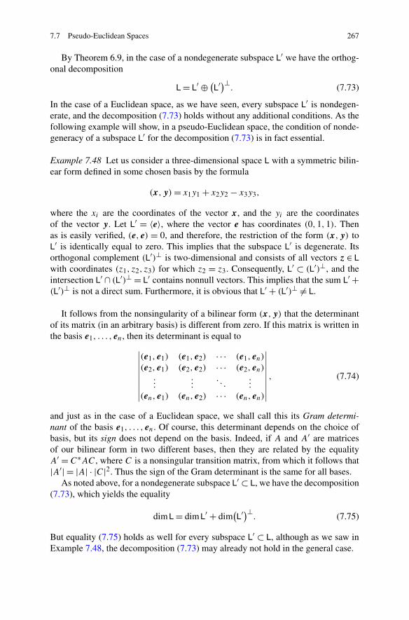
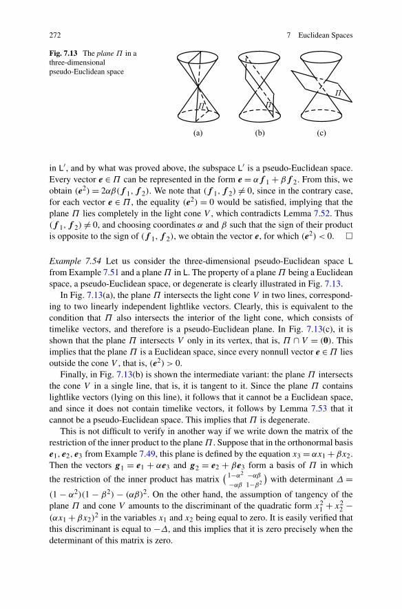
The notions entering into the definition of a vector space do not provide a way offormulating multidimensional analogues of the length of a vector, the angle betweenvectors, and volumes. Yet such concepts appear in many branches of mathematicsand physics, and we shall study such concepts in this chapter. All the vector spacesthat we shall consider here will be real (with the exception of certain special cases inwhich complex vector spaces will be considered as a means of studying real spaces).

7.1 The Definition of a Euclidean Space

Definition 7.1 A Euclidean space is a real vector space on which is defined a fixedsymmetric bilinear form whose associated quadratic form is positive definite.

The vector space itself will be denoted as a rule by L, and the fixed symmetricbilinear form will be denoted by (x,y). Such an expression is also called the innerproduct of the vectors x and y. Let us now reformulate the definition of a Euclideanspace using this terminology.

A Euclidean space is a real vector space L in which to every pair of vectors xand y there corresponds a real number (x,y) such that the following conditions aresatisfied:

(1) (x1 + x2,y) = (x1,y) + (x2,y) for all vectors x1,x2,y ∈ L.(2) (αx,y) = α(x,y) for all vectors x,y ∈ L and real number α.(3) (x,y) = (y,x) for all vectors x,y ∈ L.(4) (x,x) > 0 for x �= 0.

Properties (1)–(3) show that the function (x,y) is a symmetric bilinear form onL, and in particular, that (0,y) = 0 for every vector y ∈ L. It is only property (4) thatexpresses the specific character of a Euclidean space.

The expression (x,x) is frequently denoted by (x2); it is called the scalar squareof the vector x. Thus property (4) implies that the quadratic form corresponding tothe bilinear form (x,y) is positive definite.

I.R. Shafarevich, A.O. Remizov, Linear Algebra and Geometry,DOI 10.1007/978-3-642-30994-6_7, © Springer-Verlag Berlin Heidelberg 2013

213

http://dx.doi.org/10.1007/978-3-642-30994-6_7

214 7 Euclidean Spaces

Let us point out some obvious consequences of these definitions. For a fixed vec-tor y ∈ L, where L is a Euclidean space, conditions (1) and (2) in the definition canbe formulated in such a way that the function f y(x) = (x,y) with argument x islinear. Thus we have a mapping y �→ f y of the vector space L to L∗. Condition (4)in the definition of Euclidean space shows that the kernel of this mapping is equalto (0). Indeed, f y �= 0 for every y �= 0, since f y(y) = (y2) > 0. If the dimensionof the space L is finite, then by Theorems 3.68 and 3.78, this mapping is an iso-morphism. Moreover, we should note that in contrast to the construction used forproving Theorem 3.78, we have now constructed an isomorphism L ∼→ L∗ withoutusing the specific choice of a basis in L. Thus we have a certain natural isomor-phism L ∼→ L∗ defined only by the imposition of an inner product on L. In view ofthis, in the case of a finite-dimensional Euclidean space L, we shall in what followssometimes identify L and L∗. In other words, as for any bilinear form, for the in-ner product (x,y) there exists a unique linear transformation A : L → L∗ such that(x,y) = A(y)(x). The previous reasoning shows that in the case of a Euclideanspace, the transformation A is an isomorphism, and in particular, the bilinear form(x,y) is nonsingular. Let us give some examples of Euclidean spaces.

Example 7.2 The plane, in which for (x,y) is taken the well-known inner productof x and y as studied in analytic geometry, that is, the product of the vectors’ lengthsand the cosine of the angle between them, is a Euclidean space.

Example 7.3 The space Rn consisting of rows (or columns) of length n, in which

the inner product of rows x = (α1, . . . , αn) and y = (β1, . . . , βn) is defined by therelation

(x,y) = α1β1 + α2β2 + · · · + αnβn, (7.1)

is a Euclidean space.

Example 7.4 The vector space L consisting of polynomials of degree at most n

with real coefficients, defined on some interval [a, b], is a Euclidean space. For twopolynomials f (t) and g(t), their inner product is defined by the relation

(f, g) =∫ b

a

f (t)g(t) dt. (7.2)

Example 7.5 The vector space L consisting of all real-valued continuous functionson the interval [a, b] is a Euclidean space. For two such functions f (t) and g(t), weshall define their inner product by equality (7.2).

Example 7.5 shows that a Euclidean space, like a vector space, does not have tobe finite-dimensional.1 In the sequel, we shall be concerned exclusively with finite-dimensional Euclidean spaces, on which the inner product is sometimes called the

1Infinite-dimensional Euclidean spaces are usually called pre-Hilbert spaces. An especially impor-tant role in a number of branches of mathematics and physics is played by the so-called Hilbert

7.1 The Definition of a Euclidean Space 215

Fig. 7.1 Orthogonalprojection

scalar product (because the inner product of two vectors is a scalar) or dot product(because the notation x · y is frequently used instead of (x,y)).

Example 7.6 Every subspace L′ of a Euclidean space L is itself a Euclidean space ifwe define on it the form (x,y) exactly as on the space L.

In analogy with Example 7.2, we make the following definition.

Definition 7.7 The length of a vector x in a Euclidean space is the nonnegativevalue

√(x2). The length of a vector x is denoted by |x|.

We note that we have here made essential use of property (4), by which the lengthof a nonnull vector is a positive number.

Following the same analogy, it is natural to define the angle ϕ between two vec-tors x and y by the condition

cosϕ = (x,y)

|x| · |y| , 0 ≤ ϕ ≤ π. (7.3)

However, such a number ϕ exists only if the expression on the right-hand side ofequality (7.3) does not exceed 1 in absolute value. Such is indeed the case, and theproof of this fact will be our immediate objective.

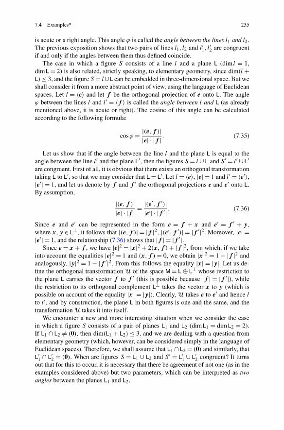
Lemma 7.8 Given a vector e �= 0, every vector x ∈ L can be expressed in the form

x = αe + y, (e,y) = 0, (7.4)

for some scalar α and vector y ∈ L; see Fig. 7.1.

Proof Setting y = x −αe, we obtain α from the condition (e,y) = 0. This is equiv-alent to (x, e) = α(e, e), which implies that α = (x, e)/|e|2. We remark that |e| �= 0,since by assumption, e �= 0. �

spaces, which are pre-Hilbert spaces that have the additional property of completeness, just forthe case of infinite dimension. (Sometimes, in the definition of pre-Hilbert space, the condition(x,x) > 0 is replaced by the weaker condition (x,x) ≥ 0.)


Definition 7.9 The vector αe from relation (7.4) is called the orthogonal projectionof the vector x onto the line 〈e〉.

Theorem 7.10 The length of the orthogonal projection of a vector x is at most itslength |x|.

Proof Indeed, since by definition, x = αe + y and (e,y) = 0, it follows that

|x|2 = (x2)= (αe + y, αe + y) = |αe|2 + |y|2 ≥ |αe|2,and this implies that

|x| ≥ |αe|. (7.5)

�

This leads directly to the following necessary theorem.

Theorem 7.11 For arbitrary vectors x and y in a Euclidean space, the followinginequality holds: ∣∣(x,y)

∣∣≤ |x| · |y|. (7.6)

Proof If one of the vectors x,y is equal to zero, then the inequality (7.6) is obvious,and is reduced to the equality 0 = 0. Now suppose that neither vector is the nullvector. In this case, let us denote by αy the orthogonal projection of the vectorx onto the line 〈y〉. Then by (7.4), we have the relationship x = αy + z, where(y,z) = 0. From this we obtain the equality

(x,y) = (αy + z,y) = (αy,y) = α|y|2.This means that |(x,y)| = |α| · |y|2 = |αy| · |y|. But by Theorem 7.10, we have

the inequality |αy| ≤ |x|, and consequently, |(x,y)| ≤ |x| · |y|. �

Inequality (7.6) goes by a number of names, but it is generally known as theCauchy–Schwarz inequality. From it we can derive the well-known triangle inequal-

ity from elementary geometry. Indeed, suppose that the vectors x = −→AB , y = −→

BC,z = −→

CA correspond to the sides of a triangle ABC. Then we have the relationshipx + y + z = 0, from which with the help of (7.6) we obtain the inequality

|z|2 = (x + y,x + y) = |x|2 + 2(x,y) + |y|2 ≤ |x|2 + 2∣∣(x,y)

∣∣+ |y|2

≤ |x|2 + 2|x| · |y| + |y|2 = (|x| + |y|)2,from which clearly follows the triangle inequality |z| ≤ |x| + |y|.

Thus from Theorem 7.11 it follows that there exists a number ϕ that satisfies theequality (7.3). This number is what is called the angle between the vectors x and y.Condition (7.3) determines the angle uniquely if we assume that 0 ≤ ϕ ≤ π .


Definition 7.12 Two vectors x and y are said to be orthogonal if their inner productis equal to zero: (x,y) = 0.

Let us note that this repeats the definition given in Sect. 6.2 for a bilinear formϕ(x,y) = (x,y). By the definition given above in (7.3), the angle between orthog-onal vectors is equal to π

2 .For a Euclidean space, there is a useful criterion for the linear independence of

vectors. Let a1, . . . ,am be m vectors in the Euclidean space L.

Definition 7.13 The Gram determinant, or Gramian, of a system of vectorsa1, . . . ,am is the determinant

G(a1, . . . ,am) =

∣∣∣∣∣∣∣∣∣

(a1,a1) (a1,a2) · · · (a1,am)

(a2,a1) (a2,a2) · · · (a2,am)...

.... . .

...

(am,a1) (am,a2) · · · (am,am)

∣∣∣∣∣∣∣∣∣. (7.7)

Theorem 7.14 If the vectors a1, . . . ,am are linearly dependent, then the Gram de-terminant G(a1, . . . ,am) is equal to zero, while if they are linearly independent,then G(a1, . . . ,am) > 0.

Proof If the vectors a1, . . . ,am are linearly dependent, then as was shown inSect. 3.2, one of the vectors can be expressed as a linear combination of the oth-ers. Let it be the vector am, that is, am = α1a1 + · · · + αm−1am−1. Then from theproperties of the inner product, it follows that for every i = 1, . . . ,m, we have theequality

(am,ai ) = α1(a1,ai ) + α2(a2,ai ) + · · · + αm−1(am−1,ai ).

From this it is clear that if we subtract from the last row of the determinant (7.7), allthe previous rows multiplied by coefficients α1, . . . , αm−1, then we obtain a deter-minant with a row consisting entirely of zeros. Therefore, G(a1, . . . ,am) = 0.

Now suppose that vectors a1, . . . ,am are linearly independent. Let us consider inthe subspace L′ = 〈a1, . . . ,am〉, the quadratic form (x2). Setting x = α1a1 + · · · +αmam, we may write it in the form

((α1a1 + · · · + αmam)2)=

m∑i,j=1

αiαj (ai ,aj ).

It is easily seen that this quadratic form is positive definite, and its determinant coin-cides with the Gram determinant G(a1, . . . ,am). By Theorem 6.19, it now followsthat G(a1, . . . ,am) > 0. �

Theorem 7.14 is a broad generalization of the Cauchy–Schwarz inequality. In-deed, for m = 2, inequality (7.6) is obvious (it becomes an equality) if vectors x


and y are linearly dependent. However, if x and y are linearly independent, thentheir Gram determinant is equal to

G(x,y) =∣∣∣∣(x,x) (x,y)

(x,y) (y,y)

∣∣∣∣ .The inequality G(x,y) > 0 established in Theorem 7.14 gives us (7.6). In partic-ular, we see that inequality (7.6) becomes an equality only if the vectors x and yare proportional. We remark that this is easy to derive if we examine the proof ofTheorem 7.11.

Definition 7.15 Vectors e1, . . . , em in a Euclidean space form an orthonormal sys-tem if

(ei , ej ) = 0 for i �= j, (ei , ei ) = 1, (7.8)

that is, if these vectors are mutually orthogonal and the length of each of them isequal to 1. If m = n and the vectors e1, . . . , en form a basis of the space, then sucha basis is called an orthonormal basis.

It is obvious that the Gram determinant of an orthonormal basis is equal to 1.We shall now use the fact that a quadratic form (x2) is positive definite and

apply to it formula (6.28), in which by the definition of positive definiteness, s = n.This result can now be reformulated as an assertion about the existence of a basise1, . . . , en of the space L in which the scalar square of a vector x = α1e1 +· · ·+αnen

is equal to the sum of the squares of its coordinates, that is, (x2) = α21 + · · · + α2

n.In other words, we have the following result.

Theorem 7.16 Every Euclidean space has an orthonormal basis.

Remark 7.17 In an orthonormal basis, the inner product of x = (α1, . . . , αn) andy = (β1, . . . , βn) has a particularly simple form, given by formula (7.1). Accord-ingly, in an orthonormal basis, the scalar square of an arbitrary vector is equal to thesum of the squares of its coordinates, while its length is equal to the square root ofthe sum of the squares.

The lemma establishing the decomposition (7.4) has an important and far-reaching generalization. To formulate it, we recall that in Sect. 3.7, for every sub-space L′ ⊂ L we defined its annihilator (L′)a ⊂ L∗, while earlier in this section, weshowed that an arbitrary Euclidean space L of finite dimension can be identifiedwith its dual space L∗. As a result, we can view (L′)a as a subspace of the originalspace L. In this light, we shall call it the orthogonal complement of the subspaceL′ and denote it by (L′)⊥. If we recall the relevant definitions, we obtain that theorthogonal complement (L′)⊥ of the subspace L′ ⊂ L consists of all vectors y ∈ Lfor which the following condition holds:

(x,y) = 0 for all x ∈ L′. (7.9)


On the other hand, (L′)⊥ is the subspace (L′)⊥ϕ , defined for the case that the bilinearform ϕ(x,y) is given by ϕ(x,y) = (x,y); see p. 198.

A basic property of the orthogonal complement in a finite-dimensional Euclideanspace is contained in the following theorem.

Theorem 7.18 For an arbitrary subspace L1 of a finite-dimensional Euclideanspace L, the following holds:

L = L1 ⊕ L⊥1 . (7.10)

In the case L1 = 〈e〉, Theorem 7.18 follows from Lemma 7.8.

Proof of Theorem 7.18 In the previous chapter, we saw that every quadratic formψ(x) in some basis of a vector space L can be reduced to the canonical form (6.22),and in the case of a real vector space, to the form (6.28) for some scalars 0 ≤ s ≤ r ,where s is the index of inertia and r is the rank of the quadratic form ψ(x), orequivalently, the rank of the symmetric bilinear form ϕ(x,y) associated with ψ(x)

by the relationship (6.11). We recall that a bilinear form ϕ(x,y) is nonsingular ifr = n, where n = dim L.

The condition of positive definiteness for the form ψ(x) is equivalent to thecondition that all scalars λ1, . . . , λn in (6.22) be positive, or equivalently, that theequality s = r = n hold in formula (6.28). From this it follows that a symmetricbilinear form ϕ(x,y) associated with a positive definite quadratic form ψ(x) isnonsingular on the space L as well as on every subspace L′ ⊂ L. To complete theproof, it suffices to recall that by definition, the quadratic form (x2) associated withthe inner product (x,y) is positive definite and to use Theorem 6.9 for the bilinearform ϕ(x,y) = (x,y). �

From relationship (3.54) for the annihilator (see Sect. 3.7) or from Theorem 7.18,it follows that

dim(L1)⊥ = dim L − dim L1.

The map that is the projection of the space L onto the subspace L1 parallel to L⊥1

(see the definition on p. 103) is called the orthogonal projection of L onto L1. Thenthe projection of the vector x ∈ L onto the subspace L1 is called its orthogonalprojection onto L1. This is a natural generalization of the notion introduced aboveof orthogonal projection of a vector onto a line. Similarly, for an arbitrary subsetX ⊂ L, we can define its orthogonal projection onto L1.

The Gram determinant is connected to the notion of volume in a Euclidean space,generalizing the notion of the length of a vector.

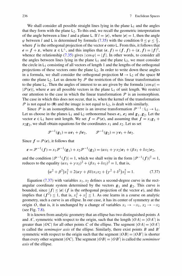
Definition 7.19 The parallelepiped spanned by vectors a1, . . . ,am is the collectionof all vectors α1a1 +· · ·+αmam for all 0 ≤ αi ≤ 1. It is denoted by Π(a1, . . . ,am).A base of the parallelepiped Π(a1, . . . ,am) is a parallelepiped spanned by anym − 1 vectors among a1, . . . ,am, for example, Π(a1, . . . ,am−1).


Fig. 7.2 Altitude of aparallelepiped

In the case of the plane (see Example 7.2), we have parallelepipeds Π(a1) andΠ(a1,a2). By definition, Π(a1) is the segment whose beginning and end coincidewith the beginning and end of the vector a1, while Π(a1,a2) is the parallelogramconstructed from the vectors a1 and a2.

We return now to the consideration of an arbitrary parallelepiped

Π(a1, . . . ,am),

and we define the subspace L1 = 〈a1, . . . ,am−1〉. To this case we may apply thenotion introduced above of orthogonal projection of the space L. By the decompo-sition (7.10), the vector am can be uniquely represented in the form am = x + y,where x ∈ L1 and y ∈ L⊥

1 . The vector y is called the altitude of the parallelepipedΠ(a1, . . . ,am) dropped to the base Π(a1, . . . ,am−1). The construction we havedescribed is depicted in Fig. 7.2 for the case of the plane.

Now we can introduce the concept of volume of a parallelepiped

Π(a1, . . . ,am),

or more precisely, its unoriented volume. This is by definition a nonnegative number,denoted by V (a1, . . . ,am) and defined by induction on m. In the case m = 1, it isequal to V (a1) = |a1|, and in the general case, V (a1, . . . ,am) is the product ofV (a1, . . . ,am−1) and the length of the altitude of the parallelepiped Π(a1, . . . ,am)

dropped to the base Π(a1, . . . ,am−1).The following is a numerical expression for the unoriented volume:

V 2(a1, . . . ,am) = G(a1, . . . ,am). (7.11)

This relationship shows the geometric meaning of the Gram determinant.Formula (7.11) is obvious for m = 1, and in the general case, it is proved by

induction on m. According to (7.10), we may represent the vector am in the formam = x + y, where x ∈ L1 = 〈a1, . . . ,am−1〉 and y ∈ L⊥

1 . Then am = α1a1 + · · · +αm−1am−1 + y. We note that y is the altitude of our parallelepiped dropped to thebase Π(a1, . . . ,am−1). Let us recall formula (7.7) for the Gram determinant andsubtract from its last column, each of the other columns multiplied by α1, . . . , αm−1.


As a result, we obtain

G(a1, . . . ,am) =

∣∣∣∣∣∣∣∣∣∣∣

(a1,a1) (a1,a2) · · · 0(a2,a1) (a2,a2) · · · 0

......

. . ....

(am−1,a1) (am−1,a2) · · · 0(am,a1) (am,a2) · · · (y,am)

∣∣∣∣∣∣∣∣∣∣∣, (7.12)

and moreover, (y,am) = (y,y) = |y|2, since y ∈ L⊥1 .

Expanding the determinant (7.12) along its last column, we obtain the equality

G(a1, . . . ,am) = G(a1, . . . ,am−1)|y|2.Let us recall that by construction, y is the altitude of the parallelepiped Π(a1, . . . ,

am) dropped to the base Π(a1, . . . ,am−1). By the induction hypothesis, we haveG(a1, . . . ,am−1) = V 2(a1, . . . ,am−1), and this implies

G(a1, . . . ,am) = V 2(a1, . . . ,am−1)|y|2 = V 2(a1, . . . ,am).

Thus the concept of unoriented volume that we have introduced differs from thevolume and area about which we spoke in Sects. 2.1 and 2.6, since the unorientedvolume cannot assume negative values. This explains the term “unoriented.” Weshall now formulate a second way of looking at the volume of a parallelepiped,one that generalizes the notions of volume and area about which we spoke earlierand differs from unoriented volume by the sign ±1. By Theorem 7.14, of interestis only the case in which the vectors a1, . . . ,am are linearly independent. Then wemay consider the space L = 〈a1, . . . ,am〉 with basis a1, . . . ,am.

Thus we are given n vectors a1, . . . ,an, where n = dim L. We consider the matrixA, whose j th column consists of the coordinates of the vector aj relative to someorthonormal basis e1, . . . , en:

A =

⎛⎜⎜⎜⎝

a11 a12 · · · a1n

a21 a22 · · · a2n

......

. . ....

an1 an2 · · · ann

⎞⎟⎟⎟⎠ .

An easy verification shows that in the matrix A∗A, the intersection of the ith rowand j th column contains the element (ai ,aj ). This implies that the determinant ofthe matrix A∗A is equal to G(a1, . . . ,an), and in view of the equalities |A∗A| =|A∗| · |A| = |A|2, we obtain |A|2 = G(a1, . . . ,an). On the other hand, from formula(7.11), it follows that G(a1, . . . ,an) = V 2(a1, . . . ,an), and this implies that

|A| = ±V (a1, . . . ,an).

The determinant of the matrix A is called the oriented volume of the n-dimensionalparallelepiped Π(a1, . . . ,an). It is denoted by v(a1, . . . ,an). Thus the oriented and


unoriented volumes are related by the equality

V (a1, . . . ,an) = ∣∣v(a1, . . . ,an)∣∣.

Since the determinant of a matrix does not change under the transpose operation,it follows that v(a1, . . . ,an) = |A∗|. In other words, for computing the orientedvolume, one may write the coordinates of the generators of the parallelepiped ai notin the columns of the matrix, but in the rows, which is sometimes more convenient.

It is obvious that the sign of the oriented volume depends on the choice of or-thonormal basis e1, . . . , en. This dependence is suggested by the term “oriented.”We shall have more to say about this in Sect. 7.3.

The volume possesses some important properties.

Theorem 7.20 Let C : L → L be a linear transformation of the Euclidean space Lof dimension n. Then for any n vectors a1, . . . ,an in this space, one has the rela-tionship

v(C(a1), . . . ,C(an)

)= |C|v(a1, . . . ,an). (7.13)

Proof We shall choose an orthonormal basis of the space L. Suppose that the trans-formation C has matrix C in this basis and that the coordinates α1, . . . , αn of anarbitrary vector a are related to the coordinates β1, . . . , βn of its image C(a) bythe relationship (3.25), or in matrix notation, (3.27). Let A be the matrix whosecolumns consist of the coordinates of the vectors a1, . . . ,an, and let A′ be the ma-trix whose columns consist of the coordinates of the vectors C(a1), . . . ,C(an). Thenit is obvious that we have the relationship A′ = CA, from which it follows that|A′| = |C| · |A|.

To complete the proof, it remains to note that |C| = |C|, and by the def-inition of oriented volume, we have the equalities v(a1, . . . ,an) = |A| andv(C(a1), . . . ,C(an)) = |A′|. �

It follows from this theorem, of course, that

V(C(a1), . . . ,C(an)

)= ∣∣|A|∣∣V (a1, . . . ,an), (7.14)

where ||A|| denotes the absolute value of the determinant of the matrix A.Using the concepts introduced thus far, we may define an analogue of the volume

V (M) for a very broad class of sets M containing all the sets actually encounteredin mathematics and physics. This is the subject of what is called measure theory, butsince it is a topic that is rather far removed from linear algebra, it will not concernus here. Let us note only that the important relationship (7.14) remains valid here:

V(C(M)

)= ∣∣|A|∣∣V (M). (7.15)

An interesting example of a set in an n-dimensional Euclidean space is the ball B(r)

of radius r , namely the set of all vectors x ∈ L such that |x| ≤ r . The set of vectorsx ∈ L for which |x| = r is called the sphere S(r) of radius r . From the relationship(7.15) it follows that V (B(r)) = Vnr

n, where Vn = V (B(1)). The calculation of the

7.2 Orthogonal Transformations 223

interesting geometric constant Vn is a question from analysis, related to the theoryof the gamma function Γ . Here we shall simply quote the result:

Vn = πn/2

Γ (n/2 + 1).

It follows from the theory of the gamma function that if n is an even number(n = 2m), then Vn = πm/m!, and if n is odd (n = 2m + 1), then Vn = 2m+1πm/(1 ·3 · · · (2m + 1)).

7.2 Orthogonal Transformations

Let L1 and L2 be Euclidean spaces of the same dimension with inner products(x,y)1 and (x,y)2 defined on them. We shall denote the length of a vector x inthe spaces L1 and L2 by |x|1 and |x|2, respectively.

Definition 7.21 An isomorphism of Euclidean spaces L1 and L2 is an isomorphismA : L1 → L2 of the underlying vector spaces that preserves the inner product, thatis, for arbitrary vectors x,y ∈ L1, the following relationship holds:

(x,y)1 = (A(x),A(y))

2. (7.16)

If we substitute the vector y = x into equality (7.16), we obtain that |x|21 =|A(x)|22, and this implies that |x|1 = |A(x)|2, that is, the isomorphism A preservesthe lengths of vectors.

Conversely, if A : L1 → L2 is an isomorphism of vector spaces that preserves thelengths of vectors, then |A(x + y)|22 = |x + y|21, and therefore,

∣∣A(x)∣∣22 + 2

(A(x),A(y)

)2 + ∣∣A(y)

∣∣22 = |x|21 + 2(x,y)1 + |y|21.

But by assumption, we also have the equalities |A(x)|2 = |x|1 and |A(y)|2 = |y|1,which implies that (x,y)1 = (A(x),A(y))2. This, strictly speaking, is a conse-quence of the fact (Theorem 6.6) that a symmetric bilinear form (x,y) is determinedby the quadratic form (x,x), and here we have simply repeated the proof given inSect. 4.1.

If the spaces L1 and L2 have the same dimension, then from the fact that the lineartransformation A : L1 → L2 preserves the lengths of vectors, it already follows thatit is an isomorphism. Indeed, as we saw in Sect. 3.5, it suffices to verify that thekernel of the transformation A is equal to (0). But if A(x) = 0, then |A(x)|2 = 0,which implies that |x|1 = 0, that is, x = 0.

Theorem 7.22 All Euclidean spaces of a given finite dimension are isomorphic toeach other.


Proof From the existence of an orthonormal basis, it follows at once that every n-dimensional Euclidean space is isomorphic to the Euclidean space in Example 7.3.Indeed, let e1, . . . , en be an orthonormal basis of a Euclidean space L. Assigning toeach vector x ∈ L the row of its coordinates in the basis e1, . . . , en, we obtain anisomorphism of the space L and the space Rn of rows of length n with inner product(7.1) (see the remarks on p. 218). It is easily seen that isomorphism is an equivalencerelation (p. xii) on the set of Euclidean spaces, and by transitivity, it follows that allEuclidean spaces of dimension n are isomorphic to each other. �

Theorem 7.22 is analogous to Theorem 3.64 for vector spaces, and its generalmeaning is the same (this is elucidated in detail in Sect. 3.5). For example, usingTheorem 7.22, we could have proved the inequality (7.6) differently from how itwas done in the preceding section. Indeed, it is completely obvious (the inequalityis reduced to an equality) if the vectors x and y are linearly dependent. If, on theother hand, they are linearly independent, then we can consider the subspace L′ =〈x,y〉. By Theorem 7.22, it is isomorphic to the plane (Example 7.2 in the previoussection), where this inequality is well known. Therefore, it must also be correct forarbitrary vectors x and y.

Definition 7.23 A linear transformation U of a Euclidean space L into itself thatpreserves the inner product, that is, satisfies the condition that for all vectors x andy,

(x,y) = (U(x),U(y)), (7.17)

is said to be orthogonal.

This is clearly a special case of an isomorphism of Euclidean spaces L1 and L2that coincide.

It is also easily seen that an orthogonal transformation U takes an orthonormalbasis to another orthonormal basis, since from the conditions (7.8) and (7.17), itfollows that U(e1), . . . ,U(en) is an orthonormal basis if e1, . . . , en is. Conversely,if a linear transformation U takes some orthonormal basis e1, . . . , en to anotherorthonormal basis, then for vectors x = α1e1 + · · · + αnen and y = β1e1 + · · · +βnen, we have

U(x) = α1U(e1) + · · · + αnU(en), U(y) = β1U(e1) + · · · + βnU(en).

Since both e1, . . . , en and U(e1), . . . ,U(en) are orthonormal bases, it follows by(7.1) that both the left- and right-hand sides of relationship (7.17) are equal to theexpression α1β1 +· · ·+αnβn, that is, relationship (7.17) is satisfied, and this impliesthat U is an orthogonal transformation.

We note the following important reformulation of this fact: for any two orthonor-mal bases of a Euclidean space, there exists a unique orthogonal transformation thattakes the first basis into the second.

Let U = (uij ) be the matrix of a linear transformation U in some orthonormalbasis e1, . . . , en. It follows from what has gone before that the transformation U is


orthogonal if and only if the vectors U(e1), . . . ,U(en) form an orthonormal basis.But by the definition of the matrix U , the vector U(ei ) is equal to

∑nk=1 ukiek , and

since e1, . . . , en is an orthonormal basis, we have

(U(ei ),U(ej )

)= u1iu1j + u2iu2j + · · · + uniunj .

The expression on the right-hand side is equal to the element cij , where the ma-trix (cij ) is equal to U∗U . This implies that the condition of orthogonality of thetransformation U can be written in the form

U∗U = E, (7.18)

or equivalently, U∗ = U−1. This equality is equivalent to

UU∗ = E, (7.19)

and can be expressed as relationships among the elements of the matrix U :

ui1uj1 + · · · + uinujn = 0 for i �= j, u2i1 + · · · + u2

in = 1. (7.20)

The matrix U satisfying the relationship (7.18) or the equivalent relationship (7.19)is said to be orthogonal.

The concept of an orthonormal basis of a Euclidean space can be interpretedmore graphically using the notion of flag (see the definition on p. 101). Namely, weassociate with an orthonormal basis e1, . . . , en the flag

(0) ⊂ L1 ⊂ L2 ⊂ · · · ⊂ Ln = L, (7.21)

in which the subspace Li is equal to 〈e1, . . . , ei〉, and the pair (Li−1,Li ) is directedin the sense that L+

i is the half-space of Li containing the vector ei . In the case of aEuclidean space, the essential fact is that we obtain a bijection between orthonormalbases and flags.

For the proof of this, we have only to verify that the orthonormal basis e1, . . . , en

is uniquely determined by its associated flag. Let this basis be associated withthe flag (7.21). If we have already constructed an orthonormal system of vectorse1, . . . , ei−1 such that Li−1 = 〈e1, . . . , ei−1〉, then we should consider the orthogo-nal complement L⊥

i−1 of the subspace Li−1 in Li . Then dim L⊥i−1 = 1 and L⊥

i−1 = 〈ei〉,where the vector ei is uniquely defined up to the factor ±1. This factor can be se-lected unambiguously based on the condition ei ∈ L+

i .An observation made earlier can now be interpreted as follows: For any two flags

Φ1 and Φ2 of a Euclidean space L, there exists a unique orthogonal transformationthat maps Φ1 to Φ2.

Our next goal will be the construction of an orthonormal basis in which a givenorthogonal transformation U has the simplest matrix possible. By Theorem 4.22,the transformation U has a one- or two-dimensional invariant subspace L′. It is clearthat the restriction of U to the subspace L′ is again an orthogonal transformation.


Let us determine first the sort of transformation that this can be, that is, what sortsof orthogonal transformations of one- and two-dimensional spaces exist.

If dim L′ = 1, then L′ = 〈e〉 for some nonnull vector e. Then U(e) = αe, whereα is some scalar. From the orthogonality of the transformation U, we obtain that

(e, e) = (αe, αe) = α2(e, e),

from which it follows that α2 = 1, and this implies that α = ±1. Consequently, ina one-dimensional space L′, there exist two orthogonal transformations: the identityE , for which E(x) = x for all vectors x, and the transformation U such that U(x) =−x. It is obvious that U = −E .

Now let dim L′ = 2, in which case L′ is isomorphic to the plane with inner product(7.1). It is well known from analytic geometry that an orthogonal transformation ofthe plane is either a rotation through some angle ϕ about the origin or a reflectionwith respect to some line l. In the first case, the orthogonal transformation U in anarbitrary orthonormal basis of the plane has matrix

(cosϕ − sinϕ

sinϕ cosϕ

). (7.22)

In the second case, the plane can be represented in the form of the direct sum L′ =l ⊕ l⊥, where l and l⊥ are lines, and for a vector x we have the decompositionx = y + z, where y ∈ l and z ∈ l⊥, while the vector U(x) is equal to y − z. If wechoose an orthonormal basis e1, e2 in such a way that the vector e1 lies on the linel, then the transformation U will have matrix

U =(

1 00 −1

). (7.23)

But we shall not presuppose this fact from analytic geometry, and instead showthat it derives from simple considerations in linear algebra. Let U have, in someorthonormal basis e1, e2, the matrix

(a b

c d

), (7.24)

that is, it maps the vector xe1 + ye2 to (ax + by)e1 + (cx + dy)e2. The fact that Upreserves the length of a vector gives the relationship

(ax + by)2 + (cx + dy)2 = x2 + y2

for all x and y. Substituting in turn (1,0), (0,1), and (1,1) for (x, y), we obtain

a2 + c2 = 1, b2 + d2 = 1, ab + cd = 0. (7.25)

From the relationship (7.19), it follows that |UU∗| = 1, and since |U∗| = |U |, it fol-lows that |U |2 = 1, and this implies that |U | = ±1. We need to consider separatelythe cases of different signs.


If |U | = −1, then the characteristic polynomial |U − tE| of the matrix (7.24) isequal to t2 − (a +d)t −1 and has positive discriminant. Therefore, the matrix (7.24)has two real eigenvalues λ1 and λ2 of opposite signs (since by Viète’s theorem,λ1λ2 = −1) and two associated eigenvectors e1 and e2. Examining the restrictionof U to the one-dimensional invariant subspaces 〈e1〉 and 〈e2〉, we arrive at theone-dimensional case considered above, from which, in particular, it follows thatthe values λ1 and λ2 are equal to ±1. Let us show that the vectors e1 and e2 areorthogonal. By the definition of eigenvectors, we have the equalities U(ei ) = λiei ,from which we have

(U(e1),U(e2)

)= (λ1e1, λ2e2) = λ1λ2(e1, e2). (7.26)

But since the transformation U is orthogonal, it follows that (U(e1),U(e2)) =(e1, e2), and from (7.26), we obtain the equality (e1, e2) = λ1λ2(e1, e2). Since λ1and λ2 have opposite signs, it follows that (e1, e2) = 0. Choosing eigenvectors e1and e2 of unit length and such that λ1 = 1 and λ2 = −1, we obtain the orthonormalbasis e1, e2 in which the transformation U has matrix (7.23). We then have the de-composition L = l ⊕ l⊥, where l = 〈e1〉 and l⊥ = 〈e2〉, and the transformation U isa reflection in the line l.

But if |U | = 1, then by relationship (7.25) for a, b, c, d , it is easy to derive, keep-ing in mind that ad − bc = 1, that there exists an angle ϕ such that a = d = cosϕ

and c = −b = sinϕ, that is, the matrix (7.24) has the form (7.22).As a basis for examining the general case, we have the following theorem.

Theorem 7.24 If a subspace L′ is invariant with respect to an orthogonal trans-formation U, then its orthogonal complement (L′)⊥ is also invariant with respectto U.

Proof We must show that for every vector y ∈ (L′)⊥, we have U(y) ∈ (L′)⊥. Ify ∈ (L′)⊥, then (x,y) = 0 for all x ∈ L′. From the orthogonality of the transforma-tion U, we obtain that (U(x),U(y)) = (x,y) = 0. Since U is a bijective mappingfrom L to L, its restriction to the invariant subspace L′ is a bijection from L′ to L′. Inother words, every vector x′ ∈ L′ can be represented in the form x′ = U(x), wherex is some other vector in L′. Consequently, (x′,U(y)) = 0 for every vector x′ ∈ L′,and this implies that U(y) ∈ (L′)⊥. �

Remark 7.25 In the proof of Theorem 7.24, we nowhere used the positive definite-ness of the quadratic form (x,x) associated with the inner product (x,y). Indeed,this theorem holds as well for an arbitrary nonsingular bilinear form (x,y). Thecondition of nonsingularity is required in order that the restriction of the transfor-mation U to an invariant subspace be a bijection, without which the theorem wouldnot be true.

Definition 7.26 Subspaces L1 and L2 of a Euclidean space are said to be mutuallyorthogonal if (x,y) = 0 for all vectors x ∈ L1 and y ∈ L2. In such a case, we write


L1 ⊥ L2. The decomposition of a Euclidean space as a direct sum of orthogonalsubspaces is called an orthogonal decomposition.

If dim L > 2, then by Theorem 4.22, the transformation U has a one- or two-dimensional invariant subspace. Thus using Theorem 7.24 as many times as neces-sary (depending on dim L), we obtain the orthogonal decomposition

L = L1 ⊕ L2 ⊕ · · · ⊕ Lk, where Li ⊥ Lj for all i �= j, (7.27)

with all subspaces Li invariant with respect to the transformation U and of dimen-sion 1 or 2.

Combining the orthonormal bases of the subspaces L1, . . . ,Lk and choosing aconvenient ordering, we obtain the following result.

Theorem 7.27 For every orthogonal transformation there exists an orthonormalbasis in which the matrix of the transformation has the block-diagonal form

⎛⎜⎜⎜⎜⎜⎜⎜⎜⎜⎜⎜⎜⎜⎜⎜⎝

1. . . 0

1−1

. . .

−1Aϕ1

0. . .

Aϕr

⎞⎟⎟⎟⎟⎟⎟⎟⎟⎟⎟⎟⎟⎟⎟⎟⎠

, (7.28)

where

Aϕi=(

cosϕi − sinϕi

sinϕi cosϕi

), (7.29)

ϕi �= πk, k ∈ Z.

Let us note that the determinants of all the matrices (7.29) are equal to 1, andtherefore, for a proper orthogonal transformation (see the definition on p. 135), thenumber of −1’s on the main diagonal in (7.28) is even, and for an improper orthog-onal transformation, that number is odd.

Let us now look at what the theorems we have proved give us in the cases n =1,2,3 familiar from analytic geometry.

For n = 1, there exist, as we have already seen, altogether two orthogonal trans-formations, namely E and −E , the first of which is proper, and the second, improper.

For n = 2, a proper orthogonal transformation is a rotation of the plane throughsome angle ϕ. In an arbitrary orthonormal basis, its matrix has the form Aϕ from(7.29), with no restriction on the angle ϕ. For the improper transformation appearing


Fig. 7.3 Reflection of theplane with respect to a line

in (7.28), the number −1 must be encountered an odd number of times, that is, once.This implies that in some orthonormal basis e1, e2, its matrix has the form

(−1 00 1

).

This transformation is a reflection of the plane with respect to the line 〈e2〉 (Fig. 7.3).Let us now consider the case n = 3. Since the characteristic polynomial of the

transformation U has odd degree 3, it must have at least one real root. This impliesthat in the representation (7.28), the number +1 or −1 must appear on the maindiagonal of the matrix.

Let us consider proper transformations first. In this case, for the matrix (7.28),we have only one possibility:

⎛⎝1 0 0

0 cosϕ − sinϕ

0 sinϕ cosϕ

⎞⎠ .

If the matrix is written in the basis e1, e2, e3, then the transformation U does notchange the points of the line l = 〈e1〉 and represents a rotation through the angle ϕ

in the plane 〈e2, e3〉. In this case, we say that the transformation U is a a rotationof the plane through the angle ϕ about the axis l. That every proper orthogonaltransformation of a three-dimensional Euclidean space possesses a “rotational axis”is a result first proved by Euler. We shall discuss the mechanical significance of thisassertion later, in connection with motions of affine spaces.

Finally, if an orthogonal transformation is improper, then in expression (7.28),we have only the possibility

⎛⎝−1 0 0

0 cosϕ − sinϕ

0 sinϕ cosϕ

⎞⎠ .

In this case, the orthogonal transformation U reduces to a rotation about the l-axiswith a simultaneous reflection with respect to the plane l⊥.


7.3 Orientation of a Euclidean Space*

In a Euclidean space, as in any real vector space, there are defined the notionsof equal and opposite orientations of two bases and orientation of the space (seeSect. 4.4). But in Euclidean spaces, these notions possess certain specific features.

Let e1, . . . , en and e′1, . . . , e

′n be two orthonormal bases of a Euclidean space L.

By general definition, they have equal orientations if the transformation from onebasis to the other is proper. This implies that for a transformation U such that

U(e1) = e′1, . . . , U(en) = e′

n,

the determinant of its matrix is positive. But in the case that both bases under consid-eration are orthonormal, the mapping U, as we know, is orthogonal, and its matrixU satisfies the relationship |U | = ±1. This implies that U is a proper transforma-tion if and only if |U | = 1, and it is improper if and only if |U | = −1. We have thefollowing analogue to Theorems 4.38–4.40 of Sect. 4.4.

Theorem 7.28 Two orthogonal transformations of a real Euclidean space can becontinuously deformed into each other if and only if the signs of their determinantscoincide.

The definition of a continuous deformation repeats here the definition given inSect. 4.4 for the set A, but now consisting only of orthogonal matrices (or trans-formations). Since the product of any two orthogonal transformations is again or-thogonal, Lemma 4.37 (p. 159) is also valid in this case, and we shall make use ofit.

Proof of Theorem 7.28 Let us show that an arbitrary proper orthogonal transfor-mation U can be continuously deformed into the identity. Since the condition ofcontinuous deformability defines an equivalence relation on the set of orthogonaltransformations, then by transitivity, the assertion of the theorem will follow for allproper transformations.

Thus we must prove that there exists a family of orthogonal transformations Ut

depending continuously on the parameter t ∈ [0,1] for which U0 = E and U1 = U.The continuous dependence of Ut implies that when it is represented in an arbitrarybasis, all the elements of the matrices of the transformations Ut are continuousfunctions of t . We note that this is a not at all obvious corollary to Theorem 4.38.Indeed, it did not guarantee us that all the intermediate transformations Ut for 0 <

t < 1 are orthogonal. A possible “bad” deformation At taking us out of the domainof orthogonal transformations is depicted as the dotted line in Fig. 7.4.

We shall use Theorem 7.27 and examine the orthonormal basis in which thematrix of the transformation U has the form (7.28). The transformation U is properif and only if the number of instances of −1 on the main diagonal of (7.28) is odd.We observe that the second-order matrix(−1 0

0 −1

)

7.3 Orientation of a Euclidean Space* 231

Fig. 7.4 Deformation takingus outside the domain oforthogonal transformations

can also be written in the form (7.29) for ϕi = π . Thus a proper orthogonal trans-formation can be written in a suitable orthonormal basis in block-diagonal form

⎛⎜⎜⎜⎝

E

Aϕ1

. . .

Aϕk

⎞⎟⎟⎟⎠ , (7.30)

where the arguments ϕi can now be taken to be any values. Formula (7.30) in factgives a continuous deformation of the transformation U into E . To maintain agree-ment with our notation, let us examine the transformations Ut having in this samebasis the matrix ⎛

⎜⎜⎜⎝

E

Atϕ1

. . .

Atϕk

⎞⎟⎟⎟⎠ . (7.31)

Then it is clear first of all that the transformation Ut is orthogonal for every t , andsecondly, that U0 = E and U1 = U. This gives us a proof of the theorem in the caseof a proper transformation.

Let us now consider improper orthogonal transformations and show that any suchtransformation V can be continuously deformed into a reflection with respect to ahyperplane, that is, into a transformation F having in some orthonormal basis thematrix

F =

⎛⎜⎜⎜⎝

−1 01

. . .

0 1

⎞⎟⎟⎟⎠ . (7.32)

Let us choose an arbitrary orthonormal basis of the vector space and suppose that inthis basis, the improper orthogonal transformation V has matrix V . Then it is obvi-ous that the transformation U with matrix U = V F in this same basis is a properorthogonal transformation. Taking into account the obvious relationship F−1 = F ,we have V = UF , that is, V = UF . We shall use the family Ut effecting a con-tinuous deformation of the proper transformation U into E . From the preceding


Fig. 7.5 Oriented length

equality, with the help of Lemma 4.37, we obtain the continuous family Vt = UtF ,where V0 = EF = F and V1 = UF = V . Thus the family Vt = UtF effects thedeformation of the improper transformation V into F . �

In analogy to what we did in Sect. 4.4, Theorem 7.28 gives us the following topo-logical result: the set of orthogonal transformations consists of two path-connectedcomponents: the proper and improper orthogonal transformations.

Exactly as in Sect. 4.4, from what we have proved, it also follows that two equallyoriented orthogonal bases can be continuously deformed into each other. That is, ife1, . . . , en and e′

1, . . . , e′n are orthogonal bases with the same orientation, then there

exists a family of orthonormal bases e1(t), . . . , en(t) depending continuously onthe parameter t ∈ [0,1] such that ei (0) = ei and ei (1) = e′

i . In other words, theconcept of orientation of a space is the same whether we define it in terms of anarbitrary basis or an orthonormal one. We shall further examine oriented Euclideanspaces, choosing an orientation arbitrarily. This choice makes it possible to speak ofpositively and negatively oriented orthonormal bases.

Now we can compare the concepts of oriented and unoriented volume. These twonumbers differ by the factor ±1 (unoriented volumes are nonnegative by definition).When the oriented volume of a parallelepiped Π(a1, . . . ,an) in a space L of dimen-sion n was introduced, we noted that its definition depends on the choice of someorthonormal basis e1, . . . , en. Since we are assuming that the space L is oriented, wecan include in the definition of oriented volume of a parallelepiped Π(a1, . . . ,an)

the condition that the basis e1, . . . , en used in the definition of v(a1, . . . ,an) bepositively oriented. Then the number v(a1, . . . ,an) does not depend on the choiceof basis (that is, it remains unchanged if instead of e1, . . . , en, we take any otherorthonormal positively oriented basis e′

1, . . . , e′n). This follows immediately from

formula (7.13) for the transformation C = U and from the fact that the transforma-tion U taking one basis to the other is orthogonal and proper, that is, |U| = 1.

We can now say that the oriented volume v(a1, . . . ,an) is positive (and conse-quently equal to the unoriented volume) if the bases e1, . . . , en and a1, . . . ,an areequally oriented, and is negative (that is, it differs from the unoriented volume by asign) if these bases have opposite orientations. For example, on the line (Fig. 7.5),the length of the segment OA is equal to 2, while the length of the segment OB isequal to −2.

Thus, we may say that for the parallelepiped Π(a1, . . . ,an), its oriented volumeis its “volume with orientation.”

If we choose a coordinate origin on the real line, then a basis of it consists ofa single vector, and vectors e1 and αe1 are equally oriented if they lie to one sideof the origin, that is, α > 0. The choice of orientation on the line, one might say,corresponds to the choice of “right” and “left.”

In the real plane, the orientation given by the basis e1, e2 is determined by the“direction of rotation” from e1 to e2: clockwise or counterclockwise. Equally ori-ented bases e1, e2 and e′

1, e′2 (Fig. 7.6(a) and (b)) can be continuously transformed

7.4 Examples* 233

Fig. 7.6 Oriented bases ofthe plane

one into the other, while oppositely oriented bases cannot even if they form equalfigures (Fig. 7.6(a) and (c)), since what is required for this is a reflection, that is, animproper transformation.

In real three-dimensional space, the orientation is defined by a basis of threeorthonormal vectors. We again meet with two opposite orientations, which are rep-resented by our right and left hands (see Fig. 7.7(a)). Another method of providingan orientation in three-dimensional space is defined by a helix (Fig. 7.7(b)). In thiscase, the orientation is defined by the direction in which the helix turns as it rises—clockwise or counterclockwise.2

7.4 Examples*

Example 7.29 By the term “figure” in a Euclidean space L we shall understand anarbitrary subset S ⊂ L. Two figures S and S′ contained in a Euclidean space M ofdimension n are said to be congruent, or geometrically identical, if there exists anorthogonal transformation U of the space M taking S to S′. We shall be interestedin the following question: When are figures S and S′ congruent, that is, when do wehave U(S) = S′?

Let us first deal with the case in which the figures S and S′ consist of collectionsof m vectors: S = (a1, . . . ,am) and S′ = (a′

1, . . . ,a′m) with m ≤ n. For S and S′

to be congruent is equivalent to the existence of an orthogonal transformation Usuch that U(ai ) = a′

i for all i = 1, . . . ,m. For this, of course, it is necessary that the

Fig. 7.7 Different orientations of three-dimensional space

2The molecules of amino acids likewise determine a certain orientation of space. In biology, thetwo possible orientations are designated by D (right = dexter in Latin) and L (left = laevus). Forsome unknown reason, they all determine the same orientation, namely the counterclockwise one.


following equality holds:

(ai ,aj ) = (a′i ,a

′j

), i, j = 1, . . . ,m. (7.33)

Let us assume that vectors a1, . . . ,am are linearly independent, and we shallthen prove that the condition (7.33) is sufficient. By Theorem 7.14, in this casewe have G(a1, . . . ,am) > 0, and by assumption, G(a′

1, . . . ,a′m) = G(a1, . . . ,am).

From this same theorem, it follows that the vectors a′1, . . . ,a

′m will also be linearly

independent.Let us set

L = 〈a1, . . . ,am〉, L′ = ⟨a′1, . . . ,a

′m

⟩, (7.34)

and consider first the case m = n. Let M = 〈a1, . . . ,am〉. We shall consider thetransformation U : M → M given by the conditions U(ai ) = a′

i for all i = 1, . . . ,m.Obviously, such a transformation is uniquely determined, and by the relationship(

U

(m∑

i=1

αiai

),U

(m∑

j=1

βjaj

))=(

m∑i=1

αia′i ,

m∑j=1

βja′j

)=

m∑i,j=1

αiβj

(a′

i ,a′j

)

and equality (7.33), it is orthogonal.Let m < n. Then we have the decomposition M = L ⊕ L⊥ = L′ ⊕ (L′)⊥, where

the subspaces L and L′ of the space M are defined by formula (7.34). By what hasgone before, there exists an isomorphism V : L → L′ such that V(ai ) = a′

i for alli = 1, . . . ,m. The orthogonal complements L⊥ and (L′)⊥ of these subspaces havedimension n − m, and consequently, are also isomorphic (Theorem 7.22). Let uschoose an arbitrary isomorphism W : L⊥ → (L′)⊥. As a result of the decompositionM = L ⊕ L⊥, an arbitrary vector x ∈ M can be uniquely represented in the form x =y + z, where y ∈ L and z ∈ L⊥. Let us define the linear transformation U : M → Mby the formula U(x) = V(y) + W(z). By construction, U(ai ) = a′

i for all i =1, . . . ,m, and a trivial verification shows that the transformation U is orthogonal.

Let us now consider the case that S = l and S′ = l′ are lines, and consequently,consist of an infinite number of vectors. It suffices to set l = 〈e〉 and l′ = 〈e′〉, where|e| = |e′| = 1, and to use the fact that there exists an orthogonal transformation Uof the space M taking e to e′. Thus any two lines are congruent.

The next case in order of increasing complexity is that in which figures S andS′ each consist of two lines: S = l1 ∪ l2 and S′ = l′1 ∪ l′2. Let us set li = 〈ei〉 andl′i = 〈e′

i〉, where |ei | = |e′i | = 1 for i = 1 and 2. Now, however, vectors e1 and e2

are no longer defined uniquely, but can be replaced by −e1 or −e2. In this case,their lengths do not change, but the inner product (e1, e2) can change their sign,that is, what remains unchanged is only their absolute value |(e1, e2)|. Based onprevious considerations, we may say that figures S and S′ are congruent if and onlyif |(e1, e2)| = |(e′

1, e′2)|. If ϕ is the angle between the vectors e1 and e2, then we

see that the lines l1 and l2 determine | cosϕ|, or equivalently the angle ϕ, for which0 ≤ ϕ ≤ π

2 . In textbooks on geometry, one often reads about two angles betweenstraight lines, the “acute” and “obtuse” angles, but we shall choose only the one that

7.4 Examples* 235

is acute or a right angle. This angle ϕ is called the angle between the lines l1 and l2.The previous exposition shows that two pairs of lines l1, l2 and l′1, l′2 are congruentif and only if the angles between them thus defined coincide.

The case in which a figure S consists of a line l and a plane L (dim l = 1,dim L = 2) is also related, strictly speaking, to elementary geometry, since dim(l +L) ≤ 3, and the figure S = l∪L can be embedded in three-dimensional space. But weshall consider it from a more abstract point of view, using the language of Euclideanspaces. Let l = 〈e〉 and let f be the orthogonal projection of e onto L. The angleϕ between the lines l and l′ = 〈f 〉 is called the angle between l and L (as alreadymentioned above, it is acute or right). The cosine of this angle can be calculatedaccording to the following formula:

cosϕ = |(e,f )||e| · |f | . (7.35)

Let us show that if the angle between the line l and the plane L is equal to theangle between the line l′ and the plane L′, then the figures S = l ∪ L and S′ = l′ ∪ L′are congruent. First of all, it is obvious that there exists an orthogonal transformationtaking L to L′, so that we may consider that L = L′. Let l = 〈e〉, |e| = 1 and l′ = 〈e′〉,|e′| = 1, and let us denote by f and f ′ the orthogonal projections e and e′ onto L.By assumption,

|(e,f )||e| · |f | = |(e′,f ′)|

|e′| · |f ′| . (7.36)

Since e and e′ can be represented in the form e = f + x and e′ = f ′ + y,where x,y ∈ L⊥, it follows that |(e,f )| = |f |2, |(e′,f ′)| = |f ′|2. Moreover, |e| =|e′| = 1, and the relationship (7.36) shows that |f | = |f ′|.

Since e = x + f , we have |e|2 = |x|2 + 2(x,f ) + |f |2, from which, if we takeinto account the equalities |e|2 = 1 and (x,f ) = 0, we obtain |x|2 = 1 − |f |2 andanalogously, |y|2 = 1 − |f ′|2. From this follows the equality |x| = |y|. Let us de-fine the orthogonal transformation U of the space M = L ⊕ L⊥ whose restriction tothe plane L carries the vector f to f ′ (this is possible because |f | = |f ′|), whilethe restriction to its orthogonal complement L⊥ takes the vector x to y (which ispossible on account of the equality |x| = |y|). Clearly, U takes e to e′ and hence l

to l′, and by construction, the plane L in both figures is one and the same, and thetransformation U takes it into itself.

We encounter a new and more interesting situation when we consider the casein which a figure S consists of a pair of planes L1 and L2 (dim L1 = dim L2 = 2).If L1 ∩ L2 �= (0), then dim(L1 + L2) ≤ 3, and we are dealing with a question fromelementary geometry (which, however, can be considered simply in the language ofEuclidean spaces). Therefore, we shall assume that L1 ∩ L2 = (0) and similarly, thatL′

1 ∩ L′2 = (0). When are figures S = L1 ∪ L2 and S′ = L′

1 ∪ L′2 congruent? It turns

out that for this to occur, it is necessary that there be agreement of not one (as in theexamples considered above) but two parameters, which can be interpreted as twoangles between the planes L1 and L2.


We shall consider all possible straight lines lying in the plane L1 and the anglesthat they form with the plane L2. To this end, we recall the geometric interpretationof the angle between a line l and a plane L. If l = 〈e〉, where |e| = 1, then the angleϕ between l and L is determined by formula (7.35) with the condition 0 ≤ ϕ ≤ π

2 ,where f is the orthogonal projection of the vector e onto L. From this, it follows thate = f + x, where x ∈ L⊥, and this implies that (e,f ) = (f ,f ) + (x,f ) = |f |2,whence the relationship (7.35) gives | cosϕ| = |f |. In other words, to consider allthe angles between lines lying in the plane L1 and the plane L2, we must considerthe circle in L1 consisting of all vectors of length 1 and the lengths of the orthogonalprojections of these vectors onto the plane L2. In order to write down these anglesin a formula, we shall consider the orthogonal projection M → L2 of the space Monto the plane L2. Let us denote by P the restriction of this linear transformationto the plane L1. Then the angles of interest to us are given by the formula | cosϕ| =|P (e)|, where e are all possible vectors in the plane L1 of unit length. We restrictour attention to the case in which the linear transformation P is an isomorphism.The case in which this does not occur, that is, when the kernel of the transformationP is not equal to (0) and the image is not equal to L2, is dealt with similarly.

Since P is an isomorphism, there is an inverse transformation P −1 : L2 → L1.Let us choose in the planes L1 and L2 orthonormal bases e1, e2 and g1,g2. Let thevector e ∈ L1 have unit length. We set f = P (e), and assuming that f = x1g1 +x2g2, we shall obtain equations for the coordinates x1 and x2. Let us set

P −1(g1) = αe1 + βe2, P −1(g2) = γ e1 + δe2.

Since f = P (e), it follows that

e = P −1(f ) = x1P−1(g1) + x2P

−1(g2) = (αx1 + γ x2)e1 + (βx1 + δx2)e2,

and the condition |P −1(f )| = 1, which we shall write in the form |P −1(f )|2 = 1,reduces to the equality (αx1 + γ x2)

2 + (βx1 + δx2)2 = 1, that is,

(α2 + β2)x2

1 + 2(αγ + βδ)x1x2 + (γ 2 + δ2)x22 = 1. (7.37)

Equation (7.37) with variables x1, x2 defines a second-degree curve in the rect-angular coordinate system determined by the vectors g1 and g2. This curve isbounded, since |f | ≤ |e| (f is the orthogonal projection of the vector e), and thisimplies that (f 2) ≤ 1, that is, x2

1 + x22 ≤ 1. As one learns in a course on analytic

geometry, such a curve is an ellipse. In our case, it has its center of symmetry at theorigin O , that is, it is unchanged by a change of variables x1 → −x1, x2 → −x2(see Fig. 7.8).

It is known from analytic geometry that an ellipse has two distinguished points A

and A′, symmetric with respect to the origin, such that the length |OA| = |OA′| isgreater than |OC| for all other points C of the ellipse. The segment |OA| = |OA′|is called the semimajor axis of the ellipse. Similarly, there exist points B and B ′symmetric with respect to the origin such that the segment |OB| = |OB ′| is shorterthan every other segment |OC|. The segment |OB| = |OB ′| is called the semiminoraxis of the ellipse.

7.4 Examples* 237

Fig. 7.8 Ellipse described byequation (7.37)

Let us recall that the length of an arbitrary line segment |OC|, where C is anypoint on the ellipse, gives us the value cosϕ, where ϕ is the angle between a certainline contained in L1 and the plane L2. From this it follows that cosϕ attains itsmaximum for one value of ϕ, while for some other value of ϕ it attains its minimum.Let us denote these angles by ϕ1 and ϕ2 respectively. By definition, 0 ≤ ϕ1 ≤ ϕ2 ≤π2 . It is these two angles that are called the angles between the planes L1 and L2.

The case that we have omitted, in which the transformation P has a nonnullkernel, reduces to the case in which the ellipse depicted in Fig. 7.8 shrinks to a linesegment.

It now remains for us to check that if both angles between the planes (L1,L2)

are equal to the corresponding angles between the planes (L′1,L′

2), then the figuresS = L1 ∪ L2 and S′ = L′

1 ∪ L′2 will be congruent, that is, there exists an orthogonal

transformation U taking the plane Li into L′i , i = 1,2.

Let ϕ1 and ϕ2 be the angles between L1 and L2, equal, by hypothesis, to the anglesbetween L′

1 and L′2. Reasoning as previously (in the case of the angle between a line

and a plane), we can find an orthogonal transformation that takes L2 to L′2. This

implies that we may assume that L2 = L′2. Let us denote this plane by L. Here, of

course, the angles ϕ1 and ϕ2 remain unchanged. Let cosϕ1 ≤ cosϕ2 for the pair ofplanes L1 and L. This implies that cosϕ1 and cosϕ2 are the lengths of the semiminorand semimajor axes of the ellipse that we considered above. This is also the case forthe pair of planes L′

1 and L. By construction, this means that cosϕ1 = |f 1| = |f ′1|

and cosϕ2 = |f 2| = |f ′2|, where the vectors f i ∈ L are orthogonal projections of

the vectors ei ∈ L1 of length 1. Reasoning similarly, we obtain the vectors f ′i ∈ L

and e′i ∈ L′

1, i = 1,2.Since |f 1| = |f ′

1|, |f 2| = |f ′2|, and since by well-known properties of the el-

lipse, its semimajor and semiminor axes are orthogonal, we can find an orthogonaltransformation of the space M that takes f 1 to f ′

1 and f 2 to f ′2, and having done so,

assume that f 1 = f ′1 and f 2 = f ′

2. But since an ellipse is defined by its semiaxes,it follows that the ellipses C1 and C′

1 that are obtained in the plane L from the planesL1 and L′

1 simply coincide. Let us consider the orthogonal projections of the spaceM to the plane L. Let us denote by P its restriction to the plane L1, and by P ′ itsrestriction to the plane L′

1.We shall assume, as we did previously, that the transformations P : L1 → L and

P ′ : L′1 → L are isomorphisms of the corresponding linear spaces, but it is not at all

necessary that they be isomorphisms of Euclidean spaces. Let us represent this with


arrows in a commutative diagram

L1

P

��

��

V

��

L

L′1

P ′

��

(7.38)

and let us show that the transformations P and P ′ differ from each other by anisomorphism of Euclidean spaces L1 and L′

1. In other words, we claim that the trans-formation V = (P ′)−1P is an isomorphism of the Euclidean spaces L1 and L′

1.As the product of isomorphisms of linear spaces, the transformation V is also an

isomorphism, that is, a bijective linear transformation. It remains for us to verify thatV preserves the inner product. As noted above, to do this, it suffices to verify thatV preserves the lengths of vectors. Let x be a vector in L. If x = 0, then the vectorV(x) is equal to 0 by the linearity of V , and the assertion is obvious. If x �= 0, thenwe set e = α−1x, where α = |x|, and then |e| = 1. The vector P (e) is containedin the ellipse C in the plane L. Since C = C′, it follows that P (e) = P ′(e′), wheree′ is some vector in the plane L′

1 and |e′| = 1. From this we obtain the equality(P ′)−1P (e) = e′, that is, V(e) = e′ and |e′| = 1, which implies that |V(x)| = α =|x|, which is what we had to prove.

We shall now consider a basis of the plane L consisting of vectors f 1 and f 2 ly-ing on the semimajor and semiminor axes of the ellipse C = C′, and augment it withvectors e1, e2, where P (ei ) = f i . We thereby obtain four vectors e1, e2,f 1,f 2 inthe space L1 + L (it is easily verified that they are linearly independent). Similarly,in the space L′

1 + L, we shall construct four vectors e′1, e

′2,f 1,f 2. We shall show

that there exists an orthogonal transformation of the space M taking the first set offour vectors into the second. To do so, it suffices to prove that the inner products ofthe associated vectors (in the order in which we have written them) coincide. Herewhat is least trivial is the relationship (e′

1, e′2) = (e1, e2), but it follows from the fact

that e′i = V(ei ), where V is an isomorphism of the Euclidean spaces L1 and L′

1. Therelationship (e′

1,f 1) = (e1,f 1) is a consequence of the fact that f 1 is an orthog-onal projection, (e1,f 1) = |f 1|2, and similarly, (e′

1,f 1) = |f 1|2. The remainingrelationships are even more obvious.

Thus the figures S = L1 ∪ L2 and S′ = L′1 ∪ L′

2 are congruent if and only if bothangles between the planes L1,L2 and L′

1,L′2 coincide. With the help of theorems

to be proved in Sect. 7.5, it will be easy for the reader to investigate the case of apair of subspaces L1,L2 ⊂ M of arbitrary dimension. In this case, the answer to thequestion whether two pairs of subspaces S = L1 ∪L2 and S′ = L′

1 ∪L′2 are congruent

is determined by the agreement of two finite sets of numbers that can be interpretedas “angles” between the subspaces L1,L2 and L′

1,L′2.

7.4 Examples* 239

Example 7.30 When the senior of the two authors of this textbook gave the courseon which it is based (this was probably in 1952 or 1953) at Moscow State Uni-versity, he told his students about a question that had arisen in the work of A.N.Kolmogorov, A.A. Petrov, and N.V. Smirnov, the answer to which in one particularcase had been obtained by A.I. Maltsev. This question was presented by the pro-fessor as an example of an unsolved problem that had been worked on by notedmathematicians yet could be formulated entirely in the language of linear algebra.At the next lecture, that is, a week later, one of the students in the class came up tohim and said that he had found a solution to the problem.3

The question posed by A.N. Kolmogorov et al. was this: In a Euclidean spaceL of dimension n, we are given n nonnull mutually orthogonal vectors x1, . . . ,xn,that is, (xi ,xj ) = 0 for all i �= j , i, j = 1, . . . , n. For what values m < n does thereexist an m-dimensional subspace M ⊂ L such that the orthogonal projections of thevectors x1, . . . ,xn to it all have the same length? A.I. Maltsev showed that if allthe vectors x1, . . . ,xn have the same length, then there exists such a subspace M ofeach dimension m < n.

The general case is approached as follows. Let us set |xi | = αi and assume thatthere exists an m-dimensional subspace M such that the orthogonal projections of allvectors xi to it have the same length α. Let us denote by P the orthogonal mappingto the subspace M, so that |P (xi )| = α. Let us set f i = α−1

i xi . Then the vectorsf 1, . . . ,f n form an orthonormal basis of the space L. Conversely, let us select in Lan orthonormal basis e1, . . . , en such that the vectors e1, . . . , em form a basis in M,that is, for the decomposition

L = M ⊕ M⊥, (7.39)

we join the orthonormal basis e1, . . . , em of the subspace M to the orthonormal basisem+1, . . . , en of the subspace M⊥.

Let f i =∑nk=1 ukiek . Then we can interpret the matrix U = (uki) as the ma-

trix of the linear transformation U, written in terms of the basis e1, . . . , en, takingvectors e1, . . . , en to vectors f 1, . . . ,f n. Since both sets of vectors e1, . . . , en andf 1, . . . ,f n are orthonormal bases, it follows that U is an orthogonal transforma-tion, in particular, by formula (7.18), satisfying the relationship

UU∗ = E. (7.40)

From the decomposition (7.39) we see that every vector f i can be uniquely rep-resented in the form of a sum f i = ui + vi , where ui ∈ M and vi ∈ M⊥. By defi-nition, the orthogonal projection of the vector f i onto the subspace M is equal toP (f i ) = ui . By construction of the basis e1, . . . , en, it follows that

P (f i ) =m∑

k=1

ukiek.

3It was published as L.B. Nisnevich, V.I. Bryzgalov, “On a problem of n-dimensional geometry,”Uspekhi Mat. Nauk 8:4(56) (1953), 169–172.


By assumption, we have the equalities |P (f i )|2 = |P (α−1i xi )|2 = α2α−2

i , whichin coordinates assume the form

m∑k=1

u2ki = α2α−2

i , i = 1, . . . , n.

If we sum these relationships for all i = 1, . . . , n and change the order of summationin the double sum, then taking into account the relationship (7.40) for the orthogonalmatrix U , we obtain the equality

α2n∑

i=1

α−2i =

n∑i=1

m∑k=1

u2ki =

m∑k=1

n∑i=1

u2ki = m, (7.41)

from which it follows that α can be expressed in terms of α1, . . . , αn, and m by theformula

α2 = m

(n∑

i=1

α−2i

)−1

. (7.42)

From this, in view of the equalities |P (f i )|2 = |P (α−1i xi )|2 = α2α−2

i , we ob-tain the expressions

∣∣P (f i )∣∣2 = m

(α2

i

n∑i=1

α−2i

)−1

, i = 1, . . . , n.

By Theorem 7.10, we have |P (f i )| ≤ |f i |, and since by construction, |f i | = 1, weobtain the inequalities

m

(α2

i

n∑i=1

α−2i

)−1

≤ 1, i = 1, . . . , n,

from which it follows that

α2i

n∑i=1

α−2i ≥ m, i = 1, . . . , n. (7.43)

Thus the inequalities (7.43) are necessary for the solvability of the problem. Letus show that they are also sufficient.

Let us consider first the case m = 1. We observe that in this situation, the in-equalities (7.43) are automatically satisfied for an arbitrary collection of positivenumbers α1, . . . , αn. Therefore, for an arbitrary system of mutually orthogonal vec-tors x1, . . . ,xn in L, we must produce a line M ⊂ L such that the orthogonal projec-tions of all these vectors onto it have the same length. For this, we shall take as such

7.4 Examples* 241

a line M = 〈y〉 with the vectors

y =n∑

i=1

(α1 · · ·αn)2

α2i

xi ,

where as before, α2i = (xi ,xi ). Since (xi ,y)

|y|2 y ∈ M and (xi − (xi ,y)

|y|2 y,y) = 0, it fol-lows that the orthogonal projection of the vector xi onto the line M is equal to

P (xi ) = (xi ,y)

|y|2 y.

Clearly, the length of each such projection

∣∣P (xi )∣∣= |(xi ,y)|

|y| = (α1 · · ·αn)2

|y|does not depend on the index of the vector xi . Thus we have proved that for anarbitrary system of n nonnull mutually orthogonal vectors in an n-dimensional Eu-clidean space, there exists a line such that the orthogonal projections of all vectorsonto it have the same length.

To facilitate understanding in what follows, we shall use the symbol P(m,n)

to denote the following assertion: If the lengths α1, . . . , αn of a system of mutu-ally orthogonal vectors x1, . . . ,xn in an n-dimensional Euclidean space L satisfycondition (7.43), then there exists an m-dimensional subspace M ⊂ L such that theorthogonal projections P (x1), . . . ,P (xn) of the vectors x1, . . . ,xn onto it have thesame length α, expressed by the formula (7.42). Using this convention, we may saythat we have proved the assertion P(1, n) for all n > 1.

Before passing to the case of arbitrary m, let us recast the problem in a moreconvenient form. Let β1, . . . , βn be arbitrary numbers satisfying the following con-dition:

β1 + · · · + βn = m, 0 < βi ≤ 1, i = 1, . . . , n. (7.44)

Let us denote by P ′(m,n) the following assertion: In the Euclidean space L thereexist an orthonormal basis g1, . . . ,gn and an m-dimensional subspace L′ ⊂ L suchthat the orthogonal projections P ′(gi ) of the basis vectors onto L′ have length

√βi ,

that is,∣∣P ′(gi )

∣∣2 = βi, i = 1, . . . , n.

Lemma 7.31 The assertions P(m,n) and P ′(m,n) with a suitable choice of num-bers α1, . . . , αn and β1, . . . , βn are equivalent.

Proof Let us first prove that the assertion P ′(m,n) follows from the assertionP(m,n). Here we are given a collection of numbers β1, . . . , βn satisfying the con-dition (7.44), and it is known that the assertion P(m,n) holds for arbitrary positive


numbers α1, . . . , αn satisfying condition (7.43). For the numbers β1, . . . , βn and ar-bitrary orthonormal basis g1, . . . ,gn we define vectors xi = β

−1/2i gi , i = 1, . . . , n.

It is clear that these vectors are mutually orthogonal, and furthermore, |xi | = β−1/2i .

Let us prove that the numbers αi = β−1/2i satisfy the inequalities (7.43). Indeed, if

we take into account the condition (7.44), we have

α2i

n∑i=1

α−2i = β−1

i

n∑i=1

βi = β−1i m ≥ m.

The assertion P(m,n) says that in the space L there exists an m-dimensionalsubspace M such that the lengths of the orthogonal projections of the vectors xi

onto it are equal to

∣∣P (xi )∣∣= α =

√√√√m

(n∑

i=1

α−2i

)−1

=√√√√m

(n∑

i=1

βi

)−1

= 1.

But then the lengths of the orthogonal projections of the vectors gi onto the samesubspace M are equal to |P (gi )| = |P (

√βixi )| = √

βi .Now let us prove that the assertion P ′(m,n) yields P(m,n). Here we are given

a collection of nonnull mutually orthogonal vectors x1, . . . ,xn of length |xi | = αi ,and moreover, the numbers αi satisfy the inequalities (7.43). Let us set

βi = α−2i m

(n∑

i=1

α−2i

)−1

and verify that βi satisfies conditions (7.44). The equality β1 +· · ·+βn = m clearlyfollows from the definition of the numbers βi . From the inequalities (7.43) it followsthat

α2i ≥

(m

n∑i=1

α−2i

)−1

,

and this implies that

βi = α−2i m

(n∑

i=1

α−2i

)−1

≤ 1.

The assertion P ′(m,n) says that there exist an orthonormal basis g1, . . . ,gn ofthe space L and an m-dimensional subspace L′ ⊂ L such that the lengths of theorthogonal projections of the vectors gi onto it are equal to |P ′(gi )| = √

βi . Butthen the orthogonal projections of the mutually orthogonal vectors β

−1/2i gi onto

the same subspace L′ will have the same length, namely 1.To prove the assertion P(m,n) for given vectors x1, . . . ,xn, it now suffices to

consider the linear transformation U of the space L mapping the vectors gi to

7.4 Examples* 243

U(gi ) = f i , where f i = α−1i xi . Since the bases g1, . . . ,gn and f 1, . . . ,f n are

orthonormal, it follows that U is an orthogonal transformation, and therefore, theorthogonal projections of the xi onto the m-dimensional subspace M = U(L′) havethe same length. Moreover, by what we have proved above, this length is equal to thenumber α determined by formula (7.42). This completes the proof of the lemma. �

Thanks to the lemma, we may prove the assertion P ′(m,n) instead of the asser-tion P(m,n). We shall do so by induction on m and n. We have already proved thebase case of the induction (m = 1, n > 1). The inductive step will be divided intothree parts:

(1) From assertion P ′(m,n) for 2m ≤ n + 1 we shall derive P ′(m,n + 1).(2) We shall prove that the assertion P ′(m,n) implies P ′(n,m − n).(3) We shall prove that the assertion P ′(m+1, n) for all n > m+1 is a consequence

of the assertion P ′(m′, n) for all m′ ≤ m and n > m′.Part 1: From assertion P ′(m,n) for 2m ≤ n+1, we derive P ′(m,n+1). We shall

consider the collection of positive numbers β1, . . . , βn,βn+1 satisfying conditions(7.44) with n replaced by n + 1, with 2m ≤ (n + 1). Without loss of generality, wemay assume that β1 ≥ β2 ≥ · · · ≥ βn+1. Since β1 + · · · + βn+1 = m and n + 1 ≥2m, it follows that βn + βn+1 ≤ 1. Indeed, for example for odd n, the contraryassumption would give the inequality

β1 + β2 ≥ · · · ≥ βn + βn+1︸︷︷︸(n+1)/2 sums

> 1,

from which clearly follows β1 +· · ·+βn+1 > (n + 1)/2 ≥ m, which contradicts theassumption that has been made.

Let us consider the (n + 1)-dimensional Euclidean space L and decompose it asa direct sum L = 〈e〉 ⊕ 〈e〉⊥, where e ∈ L is an arbitrary vector of length 1. By theinduction hypothesis, the assertion P ′(m,n) holds for numbers β1, . . . , βn−1 andβ = βn + βn+1 and the n-dimensional Euclidean space 〈e〉⊥. This implies that inthe space 〈e〉⊥, there exist an orthonormal basis g1, . . . ,gn and an m-dimensionalsubspace L′ such that the squares of the lengths of the orthogonal projections of thevectors gi onto L′ are equal to

∣∣P ′(gi )∣∣2 = βi, i = 1, . . . , n − 1,

∣∣P ′(gn)∣∣2 = βn + βn+1.

We shall denote by P : L → L′ the orthogonal projection of the space L ontoL′ (in this case, of course, P (e) = 0), and we construct in L an orthonormal basisg1, . . . , gn+1 for which |P (gi )|2 = βi for all i = 1, . . . , n + 1.

Let us set gi = gi for i = 1, . . . , n − 2 and gn = agn + be, gn+1 = cgn + de,where the numbers a, b, c, d are chosen in such a way that the following conditionsare satisfied:

|gn| = |gn+1| = 1, (gn, gn+1) = 0,

∣∣P (gn)∣∣2 = βn,

∣∣P (gn+1)∣∣2 = βn+1.

(7.45)


Then the system of vectors g1, . . . , gn+1 proves the assertion P ′(m,n + 1).The relationships (7.45) can be rewritten in the form

a2 + b2 = c2 + d2 = 1, ac + bd = 0,

a2(βn + βn+1) = βn, c2(βn + βn+1) = βn+1.

It is easily verified that these relationships will be satisfied if we set

b = ±c, d = ∓a, a =√

βn

βn + βn+1, c =

√βn+1

βn + βn+1.

Before proceeding to part 2, let us make the following observation.

Proposition 7.32 To prove the assertion P ′(m,n), we may assume that βi < 1 forall i = 1, . . . , n.

Proof Let 1 = β1 = · · · = βk > βk+1 ≥ · · · ≥ βn > 0. We choose in the n-dimensional vector space L an arbitrary subspace Lk of dimension k and considerthe orthogonal decomposition L = Lk ⊕ L⊥

k . We note that

1 > βk+1 ≥ · · · ≥ βn > 0 and βk+1 + · · · + βn = m − k.

Therefore, if the assertion P ′(m − k,n − k) holds for the numbers βk+1, . . . , βn,then in L⊥

k , there exist a subspace L′k of dimension m − k and an orthonormal basis

gk+1, . . . ,gn such that |P (gi )|2 = βi for i = k + 1, . . . , n, where P : L⊥k → L′

k isan orthogonal projection.

We now set L′ = Lk ⊕ L′k and choose in Lk an arbitrary orthonormal ba-

sis g1, . . . ,gk . Then if P ′ : L → L′ is the orthogonal projection, we have that|P ′(gi )|2 = 1 for i = 1, . . . , k and |P ′(gi )|2 = βi for i = k + 1, . . . , n. �

Part 2: Assertion P ′(m,n) implies assertion P ′(n,m − n). Let us consider n

numbers β1 ≥ · · · ≥ βn satisfying condition (7.44) in which the number m is re-placed by n − m. We must construct an orthogonal projection P ′ : L → L′ of then-dimensional Euclidean space L onto the (m − n)-dimensional subspace L′ andan orthonormal basis g1, . . . ,gn in L for which the conditions |P ′(gi )|2 = βi ,i = 1, . . . , n, are satisfied. By a previous observation, we may assume that all βi areless than 1. Then the numbers β ′

i = 1−βi satisfy conditions (7.44), and by assertionP ′(m,n), there exist an orthonormal projection P : L → L of the space L onto them-dimensional subspace L and an orthonormal basis g1, . . . ,gn for which the con-ditions |P (gi )|2 = β ′

i are satisfied. For the desired (m − n)-dimensional subspacewe shall take L′ = L⊥ and denote by P ′ the orthogonal projection onto L′. Then foreach i = 1, . . . , n, the equalities

gi = P (gi ) + P ′(gi ), 1 = |gi |2 = ∣∣P (gi )∣∣2 + ∣∣P ′(gi )

∣∣2 = β ′i + ∣∣P ′(gi )

∣∣2

7.5 Symmetric Transformations 245

are satisfied, from which it follows that |P ′(gi )|2 = 1 − β ′i = βi .

Part 3: Assertion P ′(m + 1, n) for all n > m + 1 is a consequence of P ′(m′, n)

for all m′ ≤ m and n > m′. By our assumption, the assertion P ′(m,n) holds inparticular for n = 2m + 1. By part 2, we may assert that P ′(m + 1,2m + 1) holds,and since 2(m + 1) ≤ (2m + 1) + 1, then by virtue of part 1, we may conclude thatP ′(m+1, n) holds for all n ≥ 2m+1. It remains to prove the assertions P ′(m+1, n)

for m + 2 ≤ n ≤ 2m. But these assertions follow from P ′(n − (m + 1), n) by part 2.It is necessary only to verify that the inequalities 1 ≤ n − (m + 1) ≤ m are satisfied,which follows directly from the assumption that m + 2 ≤ n ≤ 2m.

7.5 Symmetric Transformations

As we observed at the beginning of Sect. 7.1, for a Euclidean space L, there existsa natural isomorphism L ∼→ L∗ that allows us to identify in this case the space L∗with L. In particular, using the definition given in Sect. 3.7, we may define for anarbitrary basis e1, . . . , en of the space L the dual basis f 1, . . . ,f n of the space L bythe condition (f i , ei ) = 1, (f i , ej ) = 0 for i �= j . Thus an orthonormal basis is onethat is its own dual.

In the same way, we can assume that for an arbitrary linear transformationA : L → L, the dual transformation A∗ : L∗ → L∗ defined in Sect. 3.7 is a lineartransformation of the Euclidean space L into itself and is determined by the condi-tion (

A∗(x),y)= (x,A(y)

)(7.46)

for all vectors x,y ∈ L. By Theorem 3.81, the matrix of the linear transformation Ain an arbitrary basis of the space L and the matrix of the dual transformation A∗ inthe dual basis are transposes of each other. In particular, the matrices of the trans-formations A and A∗ in an arbitrary orthonormal basis are transposes of each other.This is in accord with the notation A∗ that we have chosen for the transpose matrix.It is easily verified also that conversely, if the matrices of transformations A and Bin some orthonormal basis are transposes of each other, then the transformations Aand B are dual.

As an example, let us consider the orthogonal transformation U, for whichby definition, the condition (U(x),U(y)) = (x,y) is satisfied. By formula(7.46), we have the equality (U(x),U(y)) = (x,U∗U(y)), from which follows(x,U∗U(y)) = (x,y). This implies that (x,U∗U(y) − y) = 0 for all vectors x,from which follows the equality U∗U(y) = y for all vectors y ∈ L. In other words,the fact that U∗U is equal to E , the identity transformation, is equivalent to theproperty of orthogonality of the transformation U. In matrix form, this is the rela-tionship (7.18).

Definition 7.33 A linear transformation A of a Euclidean space is called symmetricor self-dual if A∗ = A.


In other words, for a symmetric transformation A and arbitrary vectors x and y,the following condition must be satisfied:

(A(x),y

)= (x,A(y)), (7.47)

that is, the bilinear form ϕ(x,y) = (A(x),y) is symmetric. As we have seen, fromthis it follows that in an arbitrary orthonormal basis, the matrix of the transformationA is symmetric.

Symmetric linear transformations play a very large role in mathematics and itsapplications. Their most essential applications relate to quantum mechanics, wheresymmetric transformations of infinite-dimensional Hilbert space (see the note onp. 214) correspond to what are called observed physical quantities. We shall, how-ever, restrict our attention to finite-dimensional spaces. As we shall see in the sequel,even with this restriction, the theory of symmetric linear transformations has a greatnumber of applications.

The following theorem gives a basic property of symmetric linear transforma-tions of finite-dimensional Euclidean spaces.

Theorem 7.34 Every symmetric linear transformation of a real vector space has aneigenvector.

In view of the very large number of applications of this theorem, we shall presentthree proofs, based on different principles.

Proof of Theorem 7.34 First proof. Let A be a symmetric linear transformationof a Euclidean space L. If dim L > 2, then by Theorem 4.22, it has a one- or two-dimensional invariant subspace L′. It is obvious that the restriction of the transforma-tion A to the invariant subspace L′ is also a symmetric transformation. If dim L′ = 1,then we have L′ = 〈e〉, where e �= 0, and this implies that e is an eigenvector. Con-sequently, to prove the theorem, it suffices to show that a symmetric linear transfor-mation in the two-dimensional subspace L′ has an eigenvector. Choosing in L′ anorthonormal basis, we obtain for A a symmetric matrix in this basis:

A =(

a b

b c

).

In order to find an eigenvector of the transformation A, we must find a real root ofthe polynomial |A − tE|. This polynomial has the form

(a − t)(c − t) − b2 = t2 − (a + c)t + ac − b2

and has a real root if and only if its discriminant in nonnegative. But the discriminantof this quadratic trinomial is equal to

(a + c)2 − 4(ac − b2)= (a − c)2 + 4b2 ≥ 0,

and the proof is complete.


Second proof. The second proof is based on the complexification LC of the realvector space L. Following the construction presented in Sect. 4.3, we may extendthe transformation A to the vectors of the space LC. By Theorem 4.18, the obtainedtransformation AC : LC → LC will already have an eigenvector e ∈ LC and eigen-value λ ∈C, so that AC(e) = λe.

We shall extend the inner product (x,y) from the space L to LC so that it de-termines there a Hermitian form (see the definition on p. 210). It is clear that thiscan be accomplished in only one way: defining two vectors a1 = x1 + iy1 anda2 = x2 + iy2 of the space LC, we obtain the inner product according to the for-mula

(a1,a2) = (x1,x2) + (y1,y2) + i((y1,x2) − (x1,y2)

). (7.48)

The verification of the fact that the inner product (a1,a2) thus defined actually de-termines in LC a Hermitian form is reduced to the verification of sesquilinearity (inthis case, it suffices to consider separately the product of a vector a1 and a vector a2

by a real number and by i) and the property of being Hermitian. Here all calculationsare completely trivial, and we shall omit them.

An important new property of the inner product (a1,a2) that we have obtained isits positive definiteness, that is, like the scalar product (a,a), it is real (this followsfrom the Hermitian property) and (a,a) > 0, a �= 0 (this is a direct consequence offormula (7.48), for x1 = x2, y1 = y2). It is obvious that for the new inner productwe also have an analogue of the relationship (7.47), that is,

(AC(a1),a2

)= (a1,AC(a2)); (7.49)

in other words, the form ϕ(a1,a2) = (AC(a1),a2) is Hermitian. Let us apply (7.49)to the vectors a1 = a2 = e. Then we obtain (λe, e) = (e, λe). Taking into ac-count the Hermitian property, we have the equalities (λe, e) = λ(e, e) and (e, λe) =λ(e, e), from which it follows that λ(e, e) = λ(e, e). Since (e, e) > 0, we derivefrom this that λ = λ, that is, the number λ is real. Thus the characteristic polyno-mial |AC − tE | of the transformation AC has a real root λ. But a basis of the spaceL as a space over R is a basis of the space LC over C, and the matrix of the trans-formation AC in this basis coincides with the matrix of the transformation A. Inother words, |AC − tE | = |A − tE |, which implies that the characteristic polyno-mial |A − tE | of the transformation A has a real root λ, and this implies that thetransformation A : L → L has an eigenvector in the space L.

Third proof. The third proof rests on certain facts from analysis, which we nowintroduce. We first observe that a Euclidean space can be naturally converted into ametric space by defining the distance r(x,y) between two vectors x and y by therelationship r(x,y) = |x −y|. Thus in the Euclidean space L we have the notions ofconvergence, limit, continuous functions, and closed and bounded sets; see p. xvii.

The Bolzano–Weierstrass theorem asserts that for an arbitrary closed andbounded set X in a finite-dimensional Euclidean space L and arbitrary continu-ous function ϕ(x) on X there exists a vector x0 ∈ X at which ϕ(x) assumes its


maximum value: that is, ϕ(x0) ≥ ϕ(x) for all x ∈ X. This theorem is well knownfrom real analysis in the case that the set X is an interval of the real line. Its proof inthe general case is exactly the same and is usually presented somewhat later. Herewe shall use the theorem without offering a proof.

Let us apply the Bolzano–Weierstrass theorem to the set X consisting of all vec-tors x of the space L such that |x| = 1, that is, to the sphere of radius 1, and to thefunction ϕ(x) = (x,A(x)). This function is continuous not only on X, but also onthe entire space L. Indeed, it suffices to choose in the space L an arbitrary basis andto write down in it the inner product (x,A(x)) as a quadratic form in the coordinatesof the vector x. Of importance to us is solely the fact that as a result, we obtain apolynomial in the coordinates. After this, it suffices to use the well-known theoremthat states that the sum and product of continuous functions are continuous. Thenthe question is reduced to a verification of the fact that an arbitrary coordinate of thevector x is a continuous function of x, but this is completely obvious.

Thus the function (x,A(x)) assumes its maximum over the set X at some x0 = e.Let us denote this value by λ. Consequently, (x,A(x)) ≤ λ for every x for which|x| = 1. For every nonnull vector y, we set x = y/|y|. Then |x| = 1, and applyingto this vector the inequality above, we see that (y,A(y)) ≤ λ(y,y) for all y (thisobviously holds as well for y = 0).

Let us prove that the number λ is an eigenvalue of the transformation A. To thisend, let us write the condition that defines λ in the form

(y,A(y)

)≤ λ(y,y), λ = (e,A(e)), |e| = 1, (7.50)

for an arbitrary vector y ∈ L.Let us apply (7.50) to the vector y = e + εz, where both the scalar ε and vector

z ∈ L are thus far arbitrary. Expanding the expressions (y,A(y)) = (e + εz,A(e)+εA(z)) and (y,y) = (e + εz, e + εz), we obtain the inequality

(e,A(e)

)+ ε(e,A(z)

)+ ε(z,A(e)

)+ ε2(A(z),A(z))

≤ λ((e, e) + ε(e,z) + ε(z, e) + ε2(z,z)

).

In view of the symmetry of the transformation A, on the basis of the properties ofEuclidean spaces and recalling that (e, e) = 1, (e,A(e)) = λ, after canceling thecommon term (e,A(e)) = λ(e, e) on both sides of the above inequality, we obtain

2ε(e,A(z) − λz

)+ ε2((A(z),A(z))− λ(z,z)

)≤ 0. (7.51)

Let us now note that every expression aε + bε2 in the case a �= 0 assumes a pos-itive value for some ε. For this it is necessary to choose a value |ε| sufficientlysmall that a + bε has the same sign as a, and then to choose the appropriate signfor ε. Thus the inequality (7.51) always leads to a contradiction except in the case(e,A(z) − λz) = 0.

If for some vector z �= 0, we have A(z) = λz, then z is an eigenvector of thetransformation A with eigenvalue λ, which is what we wished to prove. But if


A(z) − λz �= 0 for all z �= 0, then the kernel of the transformation A − λE is equalto (0). From Theorem 3.68 it follows that then the transformation A − λE is anisomorphism, and its image is equal to all of the space L. This implies that for ar-bitrary u ∈ L, it is possible choose a vector z ∈ L such that u = A(z) − λz. Thentaking into account relationship (e,A(z)−λz) = 0, we obtain that an arbitrary vec-tor u ∈ L satisfies the equality (e,u) = 0. But this is impossible at least for u = e,since |e| = 1. �

The further theory of symmetric transformations is constructed on the basis ofsome very simple considerations.

Theorem 7.35 If a subspace L′ of a Euclidean space L is invariant with respectto the symmetric transformation A, then its orthogonal complement (L′)⊥ is alsoinvariant.

Proof The result is a direct consequence of the definitions. Let y be a vector in(L′)⊥. Then (x,y) = 0 for all x ∈ L′. In view of the symmetry of the transformationA, we have the relationship

(x,A(y)

)= (A(x),y),

while taking into account the invariance of L′ yields that A(x) ∈ L′. This impliesthat (x,A(y)) = 0 for all vectors x ∈ L′, that is, A(y) ∈ (L′)⊥, and this completesthe proof of the theorem. �

Combining Theorems 7.34 and 7.35 yields a fundamental result in the theory ofsymmetric transformations.

Theorem 7.36 For every symmetric transformation A of a Euclidean space L offinite dimension, there exists an orthonormal basis of this space consisting of eigen-vectors of the transformation A.

Proof The proof is by induction on the dimension of the space L. Indeed, by Theo-rem 7.34, the transformation A has at least one eigenvector e. Let us set

L = 〈e〉 ⊕ 〈e〉⊥,

where 〈e〉⊥ has dimension n − 1, and by Theorem 7.35, is invariant with respectto A. By the induction hypothesis, in the space 〈e〉⊥ there exists a required basis. Ifwe add the vector e to this basis, we obtain the desired basis in L. �

Let us discuss this result. For a symmetric transformation A, we have an or-thonormal basis e1, . . . , en consisting of eigenvectors. But to what extent is such abasis uniquely determined? Suppose the vector ei has the associated eigenvalue λi .


Then in our basis, the transformation A has matrix

A =

⎛⎜⎜⎜⎝

λ1 0 · · · 00 λ2 · · · 0...

.... . .

...

0 0 · · · λn

⎞⎟⎟⎟⎠ . (7.52)

But as we saw in Sect. 4.1, the eigenvalues of a linear transformation A coincidewith the roots of the characteristic polynomial

|A − tE | = |A − tE| =n∏

i=1

(λi − t).

Thus the eigenvalues λ1, . . . , λn of the transformation A are uniquely determined.Suppose that the distinct values among them are λ1, . . . , λk . If we assemble all thevectors of the constructed orthonormal basis that correspond to one and the sameeigenvalue λi (from the set λ1, . . . , λk of distinct eigenvalues) and consider the sub-space spanned by them, then we obviously obtain the eigensubspace Lλi

(see thedefinition on p. 138). We then have the orthogonal decomposition

L = Lλ1 ⊕ · · · ⊕ Lλk, where Lλi

⊥ Lλjfor all i �= j. (7.53)

The restriction of A to the eigensubspace Lλigives a transformation λiE , and in this

subspace, every orthonormal basis consists of eigenvectors (with eigenvalue λi ).Thus we see that a symmetric transformation A uniquely defines only the eigen-

subspace Lλi, while in each of them, one can choose an orthonormal basis as one

likes. On combining these bases, we obtain an arbitrary basis of the space L satisfy-ing the conditions of Theorem 7.36.

Let us note that every eigenvector of the transformation A lies in one of the sub-spaces Lλi

. If two eigenvectors x and y are associated with different eigenvaluesλi �= λj , then they lie in different subspaces Lλi

and Lλj, and in view of the orthog-

onality of the decomposition (7.53), they must be orthogonal. We thus obtain thefollowing result.

Theorem 7.37 The eigenvectors of a symmetric transformation corresponding todifferent eigenvalues are orthogonal.

We note that this theorem can also be easily proved by direct calculation.

Proof of Theorem 7.37 Let x and y be eigenvectors of a symmetric transformationA corresponding to distinct eigenvalues λi and λj . Let us substitute the expressionsA(x) = λix and A(y) = λjy into the equality (A(x),y) = (x,A(y)). From thiswe obtain (λi − λj )(x,y) = 0, and since λi �= λj , we have (x,y) = 0. �

Theorem 7.36 is often formulated conveniently as a theorem about quadraticforms using Theorem 6.3 from Sect. 6.1 and the possibility of identifying the space


L∗ with L if the space L is equipped with an inner product. Indeed, Theorem 6.3shows that every bilinear form ϕ on a Euclidean space L can be represented in theform

ϕ(x,y) = (x,A(y)), (7.54)

where A is the linear transformation of the space L to L∗ uniquely defined by the bi-linear form ϕ; that is, if we make the identification of L∗ with L, it is a transformationof the space L into itself.

It is obvious that the symmetry of the transformation A coincides with the sym-metry of the bilinear form ϕ. Therefore, the bijection between symmetric bilin-ear forms and linear transformations established above yields the same correspon-dence between quadratic forms and symmetric linear transformations of a Euclideanspace L. Moreover, in view of relationship (7.54), to the symmetric transformationA there corresponds the quadratic form

ψ(x) = (x,A(x)),

and every quadratic form ψ(x) has a unique representation in this form.If in some basis e1, . . . , en, the transformation A has a diagonal matrix (7.52),

then for the vector x = x1e1 + · · · + xnen, the quadratic form ψ(x) has in this basisthe canonical form

ψ(x) = λ1x21 + · · · + λnx

2n. (7.55)

Thus Theorem 7.36 is equivalent to the following.

Theorem 7.38 For any quadratic form in a finite-dimensional Euclidean space,there exists an orthonormal basis in which it has the canonical form (7.55).

Theorem 7.38 is sometimes conveniently formulated as a theorem about arbitraryvector spaces.

Theorem 7.39 For two quadratic forms in a finite-dimensional vector space, one ofwhich is positive definite, there exists a basis (not necessarily orthonormal) in whichthey both have canonical form (7.55).

In this case, we say that in a suitable basis, these quadratic forms are reduced toa sum of squares (even if there are negative coefficients λi in formula (7.55)).

Proof of Theorem 7.39 Let ψ1(x) and ψ2(x) be two such quadratic forms, one ofwhich, let it be ψ1(x), is positive definite. By Theorem 6.10, there exists, in thevector space L in question, a basis in which the form ψ1(x) has the canonical form(7.55). Since by assumption, the quadratic form ψ1(x) is positive definite, it followsthat in formula (7.55), all the numbers λi are positive, and therefore, there exists abasis e1, . . . , en of the space L in which ψ1(x) is brought into the form

ψ(x) = x21 + · · · + x2

n. (7.56)


Let us consider as the scalar product (x,y) in the space L the symmetric bilinearform ϕ(x,y), associated by Theorem 6.6 with the quadratic form ψ1(x). We therebyconvert L into a Euclidean space.

As can be seen from formulas (6.14) and (7.56), the basis e1, . . . , en for this innerproduct is orthonormal. Then by Theorem 7.38, there exists an orthonormal basise′

1, . . . , e′n of the space L in which the form ψ2(x) has canonical form (7.55). But

since the basis e′1, . . . , e

′n is orthonormal with respect to the inner product that we

defined with the help of the quadratic form ψ1(x), then in this basis, ψ1(x) as beforetakes the form (7.56), and that completes the proof of the theorem. �

Remark 7.40 It is obvious that Theorem 7.39 remains true if in its formulation wereplace the condition of positive definiteness of one of the forms by the conditionof negative definiteness. Indeed, if ψ(x) is a negative definite quadratic form, thenthe form −ψ(x) is positive definite, and both of these assume canonical form in oneand the same basis.

Without the assumption of positive (or negative) definiteness of one of thequadratic forms, Theorem 7.39 is no longer true. To prove this, let us derive onenecessary (but not sufficient) condition for two quadratic forms ψ1(x) and ψ2(x) tobe simultaneously reduced to a sum of squares. Let A1 and A2 be their matrices insome basis. If the quadratic forms ψ1(x) and ψ2(x) are simultaneously reducible tosums of squares, then in some other basis, their matrices A′

1 and A′2 will be diagonal,

that is,

A′1 =

⎛⎜⎜⎜⎝

α1 0 · · · 00 α2 · · · 0...

.... . .

...

0 0 · · · αn

⎞⎟⎟⎟⎠ , A′

2 =

⎛⎜⎜⎜⎝

β1 0 · · · 00 β2 · · · 0...

.... . .

...

0 0 · · · βn

⎞⎟⎟⎟⎠ .

Then the polynomial |A′1t +A′

2| is equal to∏n

i=1(αi t +βi), that is, it can be factoredas a product of linear factors αit +βi . But by formula (6.10) for replacing the matrixof a bilinear form through a change of basis, the matrices A1,A

′1 and A2,A

′2 are

related by

A′1 = C∗A1C, A′

2 = C∗A2C,

where C is some nonsingular matrix, that is, |C| �= 0. Therefore,∣∣A′

1t + A′2

∣∣= ∣∣C∗(A1t + A2)C∣∣= ∣∣C∗∣∣|A1t + A2||C|,

from which taking into account the equality |C∗| = |C|, we obtain the relationship

|A1t + A2| = |C|−2∣∣A′

1t + A′2

∣∣,from which it follows that the polynomial |A1t + A2| can also be factored intolinear factors. Thus for two quadratic forms ψ1(x) and ψ2(x) with matrices A1 andA2 to be simultaneously reduced each to a sum of squares, it is necessary that thepolynomial |A1t + A2| be factorable into real linear factors.


Now for n = 2 we set ψ1(x) = x21 −x2

2 and ψ2(x) = x1x2. These quadratic formsare neither positive definite nor negative definite. Their matrices have the form

A1 =(

1 00 −1

), A2 =

(0 11 0

),

and it is obvious that the polynomial |A1t +A2| = −(t2 +1) cannot be factored intoreal linear factors. This implies that the quadratic forms ψ1(x) and ψ2(x) cannotsimultaneously be reduced to sums of squares.

The question of reducing pairs of quadratic forms with complex coefficients tosums of squares (with the help of a complex linear transformation) is examined indetail, for instance, in the book The Theory of Matrices, by F.R. Gantmacher. Seethe references section.

Remark 7.41 The last proof of Theorem 7.34 that we gave makes it possible to in-terpret the largest eigenvalue λ of a symmetric transformation A as the maximumof the quadratic form (x,A(x)) on the sphere |x| = 1. Let λi be the other eigen-values, so that (x,A(x)) = λ1x

21 + · · · + λnx

2n . Then λ is the greatest among the

λi . Indeed, let us assume that the eigenvalues are numbered in descending order:λ1 ≥ λ2 ≥ · · · ≥ λn. Then

λ1x21 + · · · + λnx

2n ≤ λ1

(x2

1 + · · · + x2n

),

and the maximum value of the form (x,A(x)) on the sphere |x| = 1 is equal to λ1(it is attained at the vector with coordinates x1 = 1, x2 = · · · = xn = 0). This impliesthat λ1 = λ.

There is an analogous characteristic for the other eigenvalues λi as well, namelythe Courant–Fischer theorem, which we shall present without proof. Let us considerall possible vector subspaces L′ ⊂ L of dimension k. We restrict the quadratic form(x,A(x)) to the subspace L′ and examine its values at the intersection of L′ with theunit sphere, that is, the set of all vectors x ∈ L′ that satisfy |x| = 1. By the Bolzano–Weierstrass theorem, the restriction of the form (x,A(x)) to L′ assumes a maximumvalue λ′ at some point of the sphere, which, of course depends on the subspace L′.The Courant–Fischer theorem asserts that the smallest number thus obtained (as thesubspace L′ ranges over all subspaces of dimension k) is equal to the eigenvalueλn−k+1.

Remark 7.42 Eigenvectors are connected with the question of finding maxima andminima. Let f (x1, . . . , xn) be a real-valued differentiable function of n real vari-ables. A point at which all the derivatives of the function f with respect to thevariables (x1, . . . , xn), that is, the derivatives in all directions from this point, areequal to zero is called a critical point of the function. It is proved in real analysisthat with some natural constraints, this condition is necessary (but not sufficient) forthe function f to assume a maximum or minimum value at the point in question.Let us consider a quadratic form f (x) = (x,A(x)) on the unit sphere |x| = 1. It isnot difficult to show that for an arbitrary point on this sphere, all points sufficiently


Fig. 7.9 An ellipsoid

close to it can be written in some system of coordinates such that our function f

can be viewed as a function of these coordinates. Then the critical points of thefunction (x,A(x)) are exactly those points of the sphere that are eigenvectors ofthe symmetric transformation A.

Example 7.43 Let an ellipsoid be given in three-dimensional space with coordinatesx, y, z by the equation

x2

a2+ y2

b2+ z2

c2= 1. (7.57)

The expression on the left-hand side of (7.57) can be written in the form ψ(x) =(x,A(x)), where

x = (x, y, z), A(x) =(

x

a2,

y

b2,

z

c2

).

Let us assume that 0 < a < b < c. Then the maximum value that the quadratic formψ(x) takes on the sphere |x| = 1 is λ = 1/a2. It is attained on the vectors (±1,0,0).If |ψ(x)| ≤ λ for |x| = 1, then for an arbitrary vector y �= 0, setting x = y/|y|, weobtain |ψ(y)| ≤ λ|y|2. For the vector y = 0, this inequality is obvious. Therefore,it holds in general for all y. For |ψ(y)| = 1, it then follows that |y|2 ≥ 1/λ. Thisimplies that the shortest vector y satisfying equation (7.57) is the vector (±a,0,0).The line segments beginning at the point (0,0,0) and ending at the points (±a,0,0)

are called the semiminor axes of the ellipsoid (sometimes, this same term denotestheir length). Similarly, the smallest value that the quadratic form ψ(x) attains onthe sphere |x| = 1 is equal to 1/c2. It attains this value at vectors (0,0,±1) on theunit sphere. Line segments corresponding to vectors (0,0,±c) are called semima-jor axes of the ellipsoid. A vector (0,±b,0) corresponds to a critical point of thequadratic form ψ(x) that is neither a maximum nor a minimum. Such a point iscalled a minimax, that is, as it moves from this point in one direction, the func-tion ψ(x) will increase, while in moving in another direction it will decrease (seeFig. 7.9). The line segments corresponding to the vectors (0,±b,0) are called themedian semiaxes of the ellipsoid.

Everything presented thus far in this chapter (with the exception of Sect. 7.3on the orientation of a real Euclidean space) can be transferred verbatim to complexEuclidean spaces if the inner product is defined using the positive definite Hermitianform ϕ(x,y). The condition of positive definiteness means that for the associatedquadratic Hermitian form ψ(x) = ϕ(x,x), the inequality ψ(x) > 0 is satisfied for

7.6 Applications to Mechanics and Geometry* 255

all x �= 0. If we denote, as before, the inner product by (x,y), the last condition canbe written in the form (x,x) > 0 for all x �= 0.

The dual transformation A∗, as previously, is defined by condition (7.46). Butnow, the matrix of the transformation A∗ in an orthonormal basis is obtained fromthe matrix of the transformation A not simply by taking the transpose, but by takingthe complex conjugate of the transpose. The analogue of a symmetric transforma-tion is defined as a transformation A whose associated bilinear form (x,A(y)) isHermitian.

It is a fundamental fact that in quantum mechanics, one deals with complex space.We can formulate what was stated earlier in the following form: observed physicalquantities correspond to Hermitian forms in infinite-dimensional complex Hilbertspace.

The theory of Hermitian transformations in the finite-dimensional case is con-structed even more simply than the theory of symmetric transformations in realspaces, since there is no need to prove analogues of Theorem 7.34: we know alreadythat an arbitrary linear transformation of a complex vector space has an eigenvector.From the definition of being Hermitian, it follows that the eigenvalues of a Her-mitian transformation are real. The theorems proved in this section are valid forHermitian forms (with the same proofs).

In the complex case, a transformation U preserving the inner product is calledunitary. The reasoning carried out in Sect. 7.2 shows that for a unitary transforma-tion U, there exists an orthonormal basis consisting of eigenvectors, and all eigen-values of the transformation U are complex numbers of modulus 1.

7.6 Applications to Mechanics and Geometry*

We shall present two examples from two different areas—mechanics and geome-try—in which the theorems of the previous section play a key role. Since thesequestions will be taken up in other courses, we shall allow ourselves to be brief inboth the definitions and the proofs.

Example 7.44 Let us consider the motion of a mechanical system in a small neigh-borhood of its equilibrium position. One says that such a system possesses n degreesof freedom if in some region, its state is determined by n so-called generalized co-ordinates q1, . . . , qn, which we shall consider the coordinates of a vector q in somecoordinate system, and where we will take the origin 0 to be the equilibrium posi-tion of our system. The motion of the system determines the dependence of a vectorq on time t . We shall assume that the equilibrium position under investigation isdetermined by a strict local minimum of its potential energy Π . If this value isequal to c, and the potential energy is a function Π(q1, . . . , qn) in the generalizedcoordinates (it is assumed that it does not depend on time), then this implies thatΠ(0, . . . ,0) = c and Π(q1, . . . , qn) > c for all remaining values q1, . . . , qn close tozero. From the fact that a critical point of the function Π corresponds to the min-imum value, we may conclude that at the point 0, all partial derivatives ∂Π/∂qi


become zero. Therefore, for an expansion of the function Π(q1, . . . , qn) as a seriesin powers of the variables q1, . . . , qn at the point 0, the linear terms will be equalto zero, and we obtain the expression Π(q1, . . . , qn) = c +∑n

i,j=1 bij qiqj + · · · ,where bij are certain constants, and the ellipsis indicates terms of degree greaterthan 2. Since we are considering motions not far from the point 0, we can disregardthose values. It is in this approximation that we shall consider this problem. That is,we set

Π(q1, . . . , qn) = c +n∑

i,j=1

bij qiqj .

Since Π(q1, . . . , qn) > c for all values q1, . . . , qn not equal to zero, the quadraticform

∑ni,j=1 bij qiqj will be positive definite.

Kinetic energy T is a quadratic form in so-called generalized velocities dq1/dt,

. . . , dqn/dt , which are also denoted by q1, . . . , qn, that is,

T =n∑

i,j=1

aij qi qj , (7.58)

where aij = aji are functions of q (we assume that they do not depend on time t).Considering as we did for potential energy only those values qi close to zero, wemay replace all the functions aij in (7.58) by constants aij (0), which is what weshall now assume. Kinetic energy is always positive except in the case that all qi areequal to 0, and therefore, the quadratic form (7.58) is positive definite.

Motion in a broad class of mechanical systems (so-called natural systems) isdescribed by a rather complex system of differential equations—second-order La-grange equations:

d

dt

(∂T

∂qi

)− ∂T

∂qi

= −∂Π

∂qi

, i = 1, . . . , n. (7.59)

Application of Theorem 7.39 makes it possible to reduce these equations in thegiven situation to much simpler ones. To this end, let us find a coordinate systemin which the quadratic form

∑ni,j=1 aij xixj can be brought into the form

∑ni=1 x2

i ,

and the quadratic form∑n

i,j=1 bij xixj into the form∑n

i=1 λix2i . Then in this case,

the form∑n

i,j=1 bij xixj is positive definite, which implies that all λi are positive.In this system of coordinates (we shall again denote them by q1, . . . , qn), the systemof equations (7.59) is decomposed into the independent equations

d2qi

dt2= −λiqi, i = 1, . . . , n, (7.60)

which have the solutions qi = ci cos√

λit + di sin√

λit , where ci and di are arbi-trary constants. This shows that “small oscillations” are periodic in each coordinateqi . Since they are bounded, it follows that our equilibrium position 0 is stable. Ifwe were to examine the state of equilibrium at a point that was a critical point of


potential energy Π but not a strict minimum, then in the equations (7.60) we wouldnot be able to guarantee that all the λi were positive. Then for those i for whichλi < 0, we would obtain the solutions qi = ci cosh

√−λit + di sinh√−λit , which

can grow without bound with the growth of t . Just as for λi = 0, we would obtainan unbounded solution qi = ci + dit .

Strictly speaking, we have done only the following altogether: we have replacedthe given conditions of our problem with conditions close to them, with the resultthat the problem became much simpler. Such a procedure is usual in the theory ofdifferential equations, where it is proved that solutions to a simplified system ofequations are in a certain sense similar to the solutions of the initial system. Andmoreover, the degree of this deviation can be estimated as a function of the valuesof the terms that we have ignored. This estimation takes place in a finite interval oftime whose length also depends on the value of the ignored terms. This justifies thesimplifications that we have made.

A beautiful example, which played an important role historically, is given bylateral oscillations of a string of beads.4

Suppose we have a weightless and ideally flexible thread fixed at the ends. On itare securely fastened n beads with masses m1, . . . ,mn, and suppose they divide thethread into segments of lengths l0, l1, . . . , ln. We shall assume that in its initial state,the thread lies along the x-axis, and we shall denote by y1, . . . , yn the displacementsof the beads along the y-axis. Then the kinetic energy of this system has the form

T = 1

2

n∑i=1

miy2i .

Assuming the tension of the thread to be constant (as we may because the displace-ments are small) and equal to σ , we obtain for the potential energy the expressionΠ = σΔl, where Δl =∑n

i=0 Δli is the change in length of the entire thread, andΔli is the change in length of the portion of the thread corresponding to li . Then weknow the Δli in terms of the li :

Δli =√

l2i + (yi+1 − yi)2 − li , i = 0, . . . , n,

where y0 = yn+1 = 0. Expanding this expression as a sum in yi+1 − yi , we obtainquadratic terms

∑ni=0

12li

(yi+1 − yi)2, and we may set

Π = σ

2

n∑i=0

1

li(yi+1 − yi)

2, y0 = yn+1 = 0.

4This example is taken from Gantmacher and Krein’s book Oscillation Matrices and Kernels andSmall Vibrations of Mechanical Systems, Moscow 1950, English translation, AMS Chelsea Pub-lishing, 2002.


Thus in this case, the problem is reduced to simultaneously expressing two quadraticforms in the variables y1, . . . , yn as sums of squares:

T = 1

2

n∑i=0

miy2i , Π = σ

2

n∑i=0

1

li(yi+1 − yi)

2, y0 = yn+1 = 0.

But if the masses of all the beads are equal and they divide the thread into equalsegments, that is, mi = m and li = l/(n + 1), i = 1, . . . , n, then all the formulas canbe written in a more explicit form. In this case, we are speaking about the simulta-neous representation as the sum of squares of two forms:

T = m

2

n∑i=1

y2i , Π = σ(n + 1)

l

(n∑

i=1

y2i −

n∑i=0

yiyi+1

), y0 = yn+1 = 0.

Therefore, we must use an orthogonal transformation (preserving the form∑n

i=1 y2i )

to express as a sum of squares the form∑n

i=0 yiyi+1 with matrix

A = 1

2

⎛⎜⎜⎜⎜⎜⎜⎜⎜⎜⎜⎝

0 1 0 · · · 0 0

1 0 1. . . 0 0

0 1 0. . .

. . . 0...

. . .. . .

. . .. . .

...

0 0. . . 1 0 1

0 0 · · · 0 1 0

⎞⎟⎟⎟⎟⎟⎟⎟⎟⎟⎟⎠

.

It would have been possible to take the standard route: find the eigenvaluesλ1, . . . , λn as roots of the determinant |A − tE| and eigenvectors y from the systemof equations

Ay = λy, (7.61)

where λ = λi and y is the column of unknowns y1, . . . , yn. But it is simpler touse equations (7.61) directly. They give a system of n equations in the unknownsy1, . . . , yn:

y2 = 2λy1, y1 + y3 = 2λy2, . . . ,

yn−2 + yn = 2λyn−1, yn−1 = 2λyn,

which can be written in the form

yk−1 + yk+1 = 2λyk, k = 1, . . . , n, (7.62)

where we set y0 = yn+1 = 0. The system of equations (7.62) is called a recurrencerelation, whereby each value yk+1 is expressed in terms of the two preceding values:yk and yk−1. Thus if we know two adjacent values, then we can use relationship


(7.62) to construct all the yk . The condition y0 = yn+1 = 0 is called a boundarycondition.

Let us note that for λ = ±1, the equation (7.62) with boundary condition y0 =yn+1 = 0 has only the null solution: y0 = · · · = yn+1 = 0. Indeed, for λ = 1, weobtain

y2 = 2y1, y3 = 3y1, . . . , yn = ny1, yn+1 = (n + 1)y1,

from which by yn+1 = 0 it follows that y1 = 0, and all yk are equal to 0. Similarly,for λ = −1, we obtain

y2 = −2y1, y3 = 3y1, y4 = −4y1, . . . ,

yn = (−1)n−1ny1, yn+1 = (−1)n(n + 1)y1,

from which by yn+1 = 0 it follows as well that y1 = 0, and again all the yk are equalto zero. Thus for λ = ±1, the system of equations (7.61) has as its only solutionthe vector y = 0, which by definition, cannot be an eigenvector. In other words, thisimplies that the numbers ±1 are not eigenvalues of the matrix A.

There is a lovely formula for solving equation (7.62) with boundary conditiony0 = yn+1 = 0. Let us denote by α and β the roots of the quadratic equationz2 − 2λz + 1 = 0. By the above reasoning, λ �= ±1, and therefore, the numbersα and β are distinct and cannot equal ±1. Direct substitution shows that then forarbitrary A and B , the sequence yk = Aαk + Bβk satisfies the relationship (7.62).The coefficients A and B taken to satisfy y0 = 0, y1 are given. The following yk , aswe have seen, are determined by the relationship (7.62), and this implies that againthey are given by our formula. The conditions y0 = 0, y1 fixed give B = −A andA(α − β) = y1, whence A = y1/(α − β). Thus we obtain the expression

yk = y1

α − β

(αk − βk

). (7.63)

We now use the condition yn+1 = 0, which gives αn+1 = βn+1. Moreover, sinceα and β are roots of the polynomial z2 −2λz+1, we have αβ = 1, whence β = α−1,which implies that α2(n+1) = 1. From this (taking into account that α �= ±1), weobtain

α = cos

(πj

n + 1

)+ i sin

(πj

n + 1

),

where i is the imaginary unit, and the number j assumes the values 1, . . . , n. Againusing the equation z2 − 2λz + 1 = 0, whose roots are α and β , we obtain n distinctvalues for λ:

λj = cos

(πj

n + 1

), j = 1, . . . , n,

since j = n + 2, . . . ,2n + 1 give the same values λj . These are precisely the eigen-values of the matrix A. For the eigenvector yj of the associated eigenvalue λj , we


obtain by formula (7.63) its coordinates y1j , . . . , ynj in the form

ykj = sin

(πkj

n + 1

), k = 1, . . . , n.

These formulas were derived by d’Alembert and Daniel Bernoulli. Passing to thelimit as n → ∞, Lagrange derived from these the law of vibrations of a uniformstring.

Example 7.45 Let us consider in an n-dimensional real Euclidean space L the subsetX given by the equation

F(x1, . . . , xn) = 0 (7.64)

in some coordinate system. Such a subset X is called a hypersurface and consists ofall vectors x = (x1, . . . , xn) of the Euclidean space L whose coordinates satisfy theequation5 (7.64). Using the change-of-coordinates formula (3.36), we see that theproperty of the subset X ⊂ L being a hypersurface does not depend on the choiceof coordinates, that is, on the choice of the basis of L. Then if we assume that thebeginning of every vector is located at a single fixed point, then every vector x =(x1, . . . , xn) can be identified with its endpoint, a point of the given space. In orderto conform to more customary terminology, as we continue with this example, weshall call the vectors x of which the hypersurface X consists its points.

We shall assume that F(0) = 0 and that the function F(x1, . . . , xn) is differen-tiable in each of its arguments as many times as necessary. It is easily verified thatthis condition also does not depend on the choice of basis. Let us assume in addi-tion that 0 is not a critical point of the hypersurface X, that is, that not all partialderivatives ∂F (0)/∂xi are equal to zero. In other words, if we introduce the vectorgradF = (∂F/∂x1, . . . , ∂F/∂xn), called the gradient of the function F , then thisimplies that gradF(0) �= 0.

We shall be interested in local properties of the hypersurface X, that is, prop-erties associated with points close to 0. With the assumptions that we have made,the implicit function theorem, known from analysis, shows that near 0, the coordi-nates x1, . . . , xn of each point of the hypersurface X can be represented as a func-tion of n − 1 arguments u1, . . . , un−1, and furthermore, for each point, the valuesu1, . . . , un−1 are uniquely determined. It is possible to choose as u1, . . . , un−1 somen − 1 of the coordinates x1, . . . , xn, after determining the remaining coordinate xk

from equation (7.64), for which must be satisfied only the condition ∂F∂xk

(0) �= 0 forthe given k, which holds because of the assumption gradF(0) �= 0. The functionsthat determine the dependence of the coordinates x1, . . . , xn of a point of the hyper-plane X on the arguments u1, . . . , un−1 are differentiable at all arguments as manytimes as the original function F(x1, . . . , xn).

5The more customary point of view, when the hypersurface (for example, a curve or surface) con-sists of points, requires the consideration of an n-dimensional space consisting of points (otherwiseaffine space), which will be introduced in the following chapter.


The hyperplane defined by the equation

n∑i=1

∂F

∂xi

(0)xi = 0

is called the tangent space or tangent hyperplane to the hypersurface X at the point0 and is denoted by T0X. In the case that the basis of the Euclidean space L isorthonormal, this equation can also be written in the form (gradF(0),x) = 0. As asubspace of the Euclidean space L, the tangent space T0X is also a Euclidean space.

The set of vectors depending on the parameter t taking values on some intervalof the real line, that is, x(t) = (x1(t), . . . , xn(t)), is called a smooth curve if allfunctions xi(t) are differentiable a sufficient number of times and if for every valueof the parameter t , not all the derivatives dxi/dt are equal to zero. In analogy towhat was said above about hypersurfaces, we may visualize the curve as consistingof points A(t), where each A(t) is the endpoint of some vector x(t), while all thevectors x(t) begin at a certain fixed point O . In what follows, we shall refer to thevectors x that constitute the curve as its points.

We say that a curve γ passes through the point x0 if x(t0) = x0 for some valueof the parameter t0. It is clear that here we may always assume that t0 = 0. Indeed,let us consider a different curve x(t) = (x1(t), . . . , xn(t)), where the functions xi (t)

are equal to xi(t + t0). This can also be written in the form x(τ ) = x(t), where wehave introduced a new parameter τ related to the old one by τ = t − t0.

Generally speaking, for a curve we may make an arbitrary change of parameterby the formula t = ψ(τ), where the function ψ defines a continuously differentiablebijective mapping of one interval to another. Under such a change, a curve, consid-ered as a set of points (or vectors), will remain the same. From this it follows that oneand the same curve can be written in a variety of ways using various parameters.6

We now introduce the vector dxdt

= ( dx1dt

, . . . , dxn

dt). Suppose the curve γ passes

through the point 0 for t = 0. Then the vector p = dxdt

(0) is called a tangent vectorto the curve γ at the point 0. It depends, of course, on the choice of parameter t

defining the curve. Under a change of parameter t = ψ(τ), we have

dx

dτ= dx

dt· dt

dτ= dx

dt· ψ ′(τ ), (7.65)

and the tangent vector p is multiplied by a constant equal to the value of the deriva-tive ψ ′(0). Using this fact, it is possible to arrange things so that | dx

dt(t)| = 1 for all t

close to 0. Such a parameter is said to be natural. The condition that the curve x(t)

belong to the hyperplane (7.64) gives the equality F(x(t)) = 0, which is satisfiedfor all t . Differentiating this relationship with respect to t , we obtain that the vectorp lies in the space T0X. And conversely, an arbitrary vector contained in T0X can

6For example, the circle of radius 1 with center at the origin with Cartesian coordinates x, y can bedefined not only by the formula x = cos t , y = sin t , but also by the formula x = cos τ , y = − sin τ

(with the replacement t = −τ ), or by the formula x = sin τ , y = cos τ (replacement t = π2 − τ ).


be represented in the form dxdt

(0) for some curve x(t). This curve, of course, is notuniquely determined. Curves whose tangent vectors p are proportional are said tobe tangent at the point 0.

Let us denote by n a unit vector orthogonal to the tangent space T0X. There aretwo such vectors, n and −n, and we shall choose one of them. For example, we mayset

n = gradF

|gradF | (0). (7.66)

We define the vector d2xdt2 as d

dt( dx

dt) and set

Q =(

d2x

dt2(0),n

). (7.67)

Proposition 7.46 The value Q depends only on the vector p; namely, it is aquadratic form in its coordinates.

Proof It suffices to verify this assertion by substituting in (7.67) for the vector n,any vector proportional to it, for example, gradF(0). Since by assumption, the curvex(t) is contained in the hyperplane (7.64), it follows that F(x1(t), . . . , xn(t)) = 0.Differentiating this equality twice with respect to t , we obtain

n∑i=1

∂F

∂xi

dxi

dt= 0,

n∑i,j=1

∂2F

∂xi ∂xj

dxi

dt

dxj

dt+

n∑i=1

∂F

∂xi

d2xi

dt2= 0.

Setting here t = 0, we see that

(d2x

dt2(0),gradF(0)

)= −

n∑i,j=1

∂2F

∂xi ∂xj

(0)pipj ,

where p = (p1, . . . , pn). This proves the assertion. �

The form Q(p) is called the second quadratic form of the hypersurface. Theform (p2) is called the first quadratic form when T0X is taken as a subspace of aEuclidean space L. We observe that the second quadratic form requires the selec-tion of one of two unit vectors (n or −n) orthogonal to T0X. This is frequentlyinterpreted as the selection of one side of the hypersurface in a neighborhood of thepoint 0.

The first and second quadratic forms give us the possibility to obtain an expres-sion for the curvature of certain curves x(t) lying in the hypersurface X. Let ussuppose that a curve is the intersection of a plane L′ containing the point 0 and thehypersurface X (even if only in an arbitrarily small neighborhood of the point 0).Such a curve is called a plane section of the hypersurface. If we define the curvex(t) in such a way that t is a natural parameter, then its curvature at the point 0 is


the number

k =∣∣∣∣d

2x

dt2(0)

∣∣∣∣.We assume that k �= 0 and set

m = 1

k· d2x

dt2(0).

The vector m has length 1 by definition. It is said to be normal to the curve x(t) atthe point 0. If the curve x(t) is a plane section of the hypersurface, then x(t) lies inthe plane L′ (for all sufficiently small t), and consequently, the vector

dx

dt= lim

h→0

x(t + h) − x(t)

h

also lies in the plane L′. Therefore, this holds as well for the vector d2x/dt2, whichimplies that it holds as well for the normal m. If the curve γ is defined in terms ofthe natural parameter t , then

∣∣∣∣dx

dt

∣∣∣∣2

=(

dx

dt,dx

dt

)= 1.

Differentiating this equality with respect to t , we obtain that the vectors d2x/dt2

and dx/dt are orthogonal. Hence the normal m to the curve γ is orthogonal to anarbitrary tangent vector (for arbitrary definition of the curve γ in the form x(t) withnatural parameter t), and the vector m is defined uniquely up to sign. It is obviousthat L′ = 〈m,p〉, where p is an arbitrary tangent vector.

By definition (7.67) of the second quadratic form Q and taking into account theequality |m| = |n| = 1, we obtain the expression

Q(p) = (km,n) = k(m,n) = k cosϕ, (7.68)

where ϕ is the angle between the vectors m and n. The expression k cosϕ is denotedby k and is called the normal curvature of the hypersurface X in the direction p.We recall that here n denotes the chosen unit vector orthogonal to the tangent spaceT0X, and m is the normal to the curve to which the vector p is tangent. An analo-gous formula for an arbitrary parametric definition of the curve x(t) (where t is notnecessarily a natural parameter) also uses the first quadratic form. Namely, if τ isanother parameter, while t is a natural parameter, then by formula (7.65), now in-stead of the vector p, we obtain p′ = pψ ′(0). Since Q is a quadratic form, it followsthat Q(pψ ′(0)) = ψ ′(0)

2Q(p), and instead of formula (7.68), we now obtain

Q(p)

(p2)= k cosϕ. (7.69)


Here the first quadratic form (p2) is already involved as well as the second quadraticform Q(p), but now (7.69), in contrast to (7.68), holds for an arbitrary choice ofparameter t on the curve γ .

The point of the term normal curvature given above is the following. The sectionof the hypersurface X by the plane L′ is said to be normal if n ∈ L′. The vector ndefined by formula (7.66) is orthogonal to the tangent plane T0X. But in the plane L′there is also the vector p tangent to the curve γ , and the normal vector m orthogonalto it. Thus in the case of a normal section n = ±m, this means that in formula (7.68),the angle ϕ is equal to 0 or π . Conversely, from the equality | cosϕ| = 1, it followsthat n ∈ L′. Thus in the case of a normal section, the normal curvature k differs fromk only by the factor ±1 and is defined by the relationship

k = Q(p)

|p|2 .

Since L′ = 〈m,p〉, it follows that all normal sections correspond to straight lines inthe plane L′. For each line, there exists a unique normal section containing this line.In other words, we “rotate” the plane L′ about the vector m, considering all obtainedplanes 〈m,p〉, where p is a vector in the tangent hyperplane T0X. Thus all normalsections of the hypersurface X are obtained.

We shall now employ Theorem 7.38. In our case, it gives an orthonormal basise1, . . . , en−1 in the tangent hyperplane T0X (viewed as a subspace of the Euclideanspace L) in which the quadratic form Q(p) is brought into canonical form. In otherwords, for the vector p = u1e1 + · · · + un−1en−1, the second quadratic form takesthe form Q(p) = λ1u

21 + · · · + λn−1u

2n−1. Since the basis e1, . . . , en−1 is orthonor-

mal, we have in this case

ui

|pi | = (p, ei )

|pi | = cosϕi, (7.70)

where ϕi is the angle between the vectors p and ei . From this we obtain for thenormal curvature k of the normal section γ , the formula

k = Q(p)

|p|2 =n−1∑i=1

λi

(ui

|p|)2

=n−1∑i=1

λi cos2 ϕi, (7.71)

where p is an arbitrary tangent vector to the curve γ at the point 0. Relationships(7.70) and (7.71) are called Euler’s formula. The numbers λi are called principalcurvatures of the hypersurface X at the point 0.

In the case n = 3, the hypersurface (7.64) is an ordinary surface and has two prin-cipal curvatures λ1 and λ2. Taking into account the fact that cos2 ϕ1 + cos2 ϕ2 = 1,Euler’s formula takes the form

k = λ1 cos2 ϕ1 + λ2 cos2 ϕ2 = (λ1 − λ2) cos2 ϕ1 + λ2. (7.72)

Suppose λ1 ≥ λ2. Then from (7.72), it is clear that the normal curvature k as-sumes a maximum (equal to λ1) for cos2 ϕ1 = 1 and a minimum (equal to λ2) for

7.7 Pseudo-Euclidean Spaces 265

Fig. 7.10 Elliptic (a) and hyperbolic (b) points

cos2 ϕ1 = 0. This assertion is called the extremal property of the principal curva-tures of the surface. If λ1 and λ2 have the same sign (λ1λ2 > 0), then as can beseen from (7.72), an arbitrary normal section of a surface at a given point 0 hasits curvature of the same sign, and therefore, all normal sections have convexity inthe same direction, and near the point 0, the surface lies on one side of its tangentplane; see Fig. 7.10(a). Such points are called elliptic. If λ1 and λ2 have differ-ent signs (λ1λ2 < 0), then as can be seen from formula (7.72), there exist normalsections with opposite directions of convexity, and at points near 0, the surface is lo-cated on different sides of its tangent plane; see Fig. 7.10(b). Such points are calledhyperbolic.7

From all this discussion, it is evident that the product of principal curvaturesκ = λ1λ2 characterizes some important properties of a surface (called “internal ge-ometric properties” of the surface). This product is called the Gaussian or totalcurvature of the surface.

7.7 Pseudo-Euclidean Spaces

Many of the theorems proved in the previous sections of this chapter remain validif in the definition of Euclidean space we forgo the requirement of positive definite-ness of the quadratic form (x2) or replace it with something weaker. Without thiscondition, the inner product (x,y) does not differ at all from an arbitrary symmetricbilinear form. As Theorem 6.6 shows, it is uniquely defined by the quadratic form(x2).

We thus obtain a theory that fully coincides with the theory of quadraticforms that we presented in Chap. 6. The fundamental theorem (on bringing aquadratic form into canonical form) consists in the existence of an orthonormalbasis e1, . . . , en, that is, a basis for which (ei , ej ) = 0 for all i �= j . Then for thevector x1e1 + · · · + xnen, the quadratic form (x2) is equal to λ1x

21 + · · · + λnx

2n .

7Examples of surfaces consisting entirely of elliptic points are ellipsoids, hyperboloids of twosheets, and elliptic paraboloids, while surfaces consisting entirely of hyperbolic points includehyperboloids of one sheet and hyperbolic paraboloids.


Moreover, this is true for vector spaces and bilinear forms over an arbitrary field K

of characteristic different from 2. The concept of an isomorphism of spaces makessense also in this case; as previously, it is necessary to require that the scalar product(x,y) be preserved.

The theory of such spaces (defined up to isomorphism) with a bilinear orquadratic form is of great interest (for example, in the case K = Q, the field ofrational numbers). But here we are interested in real spaces. In this case, formula(6.28) and Theorem 6.17 (law of inertia) show that up to isomorphism, a space isuniquely defined by its rank and the index of inertia of the associated quadratic form.

We shall further restrict attention to an examination of real vector spaces with anonsingular symmetric bilinear form (x,y). Let us recall that the nonsingularity ofa bilinear form implies that its rank (that is, the rank of its matrix in an arbitrarybasis of the space) is equal to dim L. In other words, this means that its radical isequal to (0); that is, if the vector x is such that (x,y) = 0 for all vectors y ∈ L, thenx = 0 (see Sect. 6.2). For a Euclidean space, this condition follows automaticallyfrom property (4) of the definition (it suffices to set there y = x).

Formula (6.28) shows that with these conditions, there exists a basis e1, . . . , en

of the space L for which

(ei , ej ) = 0 for i �= j,(e2i

)= ±1.

Such a basis is called, as it was previously, orthonormal. In it, the form (x2) can bewritten in the form

(x2)= x2

1 + · · · + x2s − x2

s+1 − · · · − x2n,

and the number s is called the index of inertia of both the quadratic form (x2) andthe pseudo-Euclidean space L.

A new difficulty appears that was not present for Euclidean spaces if the quadraticform (x2) is neither positive nor negative definite, that is, if its index of inertia s ispositive but less than n. In this case, the restriction of the bilinear form (x,y) to thesubspace L′ ⊂ L can turn out to be singular, even if the original bilinear form (x,y)

in L was nonsingular. For example, it is clear that in L, there exists a vector x �= 0for which (x2) = 0, and then the restriction of (x,y) to a one-dimensional subspace〈x〉 is singular (identically equal to zero).

Thus let us consider a vector space L with a nonsingular symmetric bilinear form(x,y) defined on it. In this case, we shall use many concepts and much of the nota-tion used for Euclidean spaces earlier. Hence, vectors x and y are called orthogonalif (x,y) = 0. Subspaces L1 and L2 are called orthogonal if (x,y) = 0 for all vectorsx ∈ L1 and y ∈ L2, and we express this by writing L1 ⊥ L2. The orthogonal comple-ment of the subspace L′ ⊂ L with respect to the bilinear form (x,y) is denoted by(L′)⊥. However, there is an important difference from the case of Euclidean spaces,in connection with which it will be useful to give the following definition.

Definition 7.47 A subspace L′ ⊂ L is said to be nondegenerate if the bilinear formobtained by restricting the form (x,y) to L′ is nonsingular. In the contrary case, L′is said to be degenerate.


By Theorem 6.9, in the case of a nondegenerate subspace L′ we have the orthog-onal decomposition

L = L′ ⊕ (L′)⊥. (7.73)

In the case of a Euclidean space, as we have seen, every subspace L′ is nondegen-erate, and the decomposition (7.73) holds without any additional conditions. As thefollowing example will show, in a pseudo-Euclidean space, the condition of nonde-generacy of a subspace L′ for the decomposition (7.73) is in fact essential.

Example 7.48 Let us consider a three-dimensional space L with a symmetric bilin-ear form defined in some chosen basis by the formula

(x,y) = x1y1 + x2y2 − x3y3,

where the xi are the coordinates of the vector x, and the yi are the coordinatesof the vector y. Let L′ = 〈e〉, where the vector e has coordinates (0,1,1). Thenas is easily verified, (e, e) = 0, and therefore, the restriction of the form (x,y) toL′ is identically equal to zero. This implies that the subspace L′ is degenerate. Itsorthogonal complement (L′)⊥ is two-dimensional and consists of all vectors z ∈ Lwith coordinates (z1, z2, z3) for which z2 = z3. Consequently, L′ ⊂ (L′)⊥, and theintersection L′ ∩ (L′)⊥ = L′ contains nonnull vectors. This implies that the sum L′ +(L′)⊥ is not a direct sum. Furthermore, it is obvious that L′ + (L′)⊥ �= L.

It follows from the nonsingularity of a bilinear form (x,y) that the determinantof its matrix (in an arbitrary basis) is different from zero. If this matrix is written inthe basis e1, . . . , en, then its determinant is equal to

∣∣∣∣∣∣∣∣∣

(e1, e1) (e1, e2) · · · (e1, en)

(e2, e1) (e2, e2) · · · (e2, en)...

.... . .

...

(en, e1) (en, e2) · · · (en, en)

∣∣∣∣∣∣∣∣∣, (7.74)

and just as in the case of a Euclidean space, we shall call this its Gram determi-nant of the basis e1, . . . , en. Of course, this determinant depends on the choice ofbasis, but its sign does not depend on the basis. Indeed, if A and A′ are matricesof our bilinear form in two different bases, then they are related by the equalityA′ = C∗AC, where C is a nonsingular transition matrix, from which it follows that|A′| = |A| · |C|2. Thus the sign of the Gram determinant is the same for all bases.

As noted above, for a nondegenerate subspace L′ ⊂ L, we have the decomposition(7.73), which yields the equality

dim L = dim L′ + dim(L′)⊥. (7.75)

But equality (7.75) holds as well for every subspace L′ ⊂ L, although as we saw inExample 7.48, the decomposition (7.73) may already not hold in the general case.


Indeed, by Theorem 6.3, we can write an arbitrary bilinear form (x,y) in thespace L in the form (x,y) = (x,A(y)), where A : L → L∗ is some linear transfor-mation. From the nonsingularity of the bilinear form (x,y) follows the nonsingular-ity of the transformation A. In other words, the transformation A is an isomorphism,that is, its kernel is equal to (0), and in particular, for an arbitrary subspace L′ ⊂ L,we have the equality dimA(L′) = dim L′. On the other hand, we can write the or-thogonal complement (L′)⊥ in the form (A(L′))a , using the notion of the annihilatorintroduced in Sect. 3.7. On the basis of what we have said above and formula (3.54)for the annihilator, we have the relationship

dim(A(L′))a = dim L − dimA

(L′)= dim L − dim L′,

that is, dim(L′)⊥ = dim L − dim L′. We note that this argument holds for vectorspaces L defined not only over the real numbers, but over any field.

The spaces that we have examined are defined (up to isomorphism) by the indexof inertia s, which can take values from 0 to n. By what we have said above, the signof the Gram determinant of an arbitrary basis is equal to (−1)n−s . It is obvious thatif we replace the inner product (x,y) in the space L by −(x,y), we shall preserve allof its essential properties, but the index of inertia s will be replaced by n−s, whencein what follows, we shall assume that n/2 ≤ s ≤ n. The case s = n correspondsto a Euclidean space. There exists, however, a phenomenon whose explanation isat present not completely clear; the most interesting questions in mathematics andphysics were until now connected with two types of spaces: those in which the indexof inertia s is equal to n and those for which s = n − 1. The theory of Euclideanspaces (s = n) has been up till now the topic of this chapter. In the remaining part,we shall consider the other case: s = n − 1. In the sequel, we shall call such spacespseudo-Euclidean spaces (although sometimes, this term is used when (x,y) is anarbitrary nonsingular symmetric bilinear form neither positive nor negative definite,that is, with index of inertia s �= 0, n).

Thus a pseudo-Euclidean space of dimension n is a vector space L equipped witha symmetric bilinear form (x,y) such that in some basis e1, . . . , en, the quadraticform (x2) takes the form

x21 + · · · + x2

n−1 − x2n. (7.76)

As in the case of a Euclidean space, we shall, as we did previously, call such basesorthonormal.

The best-known application of pseudo-Euclidean spaces is related to the specialtheory of relativity. According to an idea put forward by Minkowski, in this theory,one considers a four-dimensional space whose vectors are called space–time events(we mentioned this earlier, on p. 86). They have coordinates (x, y, z, t), and thespace is equipped with a quadratic form x2 + y2 + z2 − t2 (here the speed of lightis assumed to be 1). The pseudo-Euclidean space thus obtained is called Minkowskispace. By analogy with the physical sense of these concepts in Minkowski space, inan arbitrary pseudo-Euclidean space, a vector x is said to be spacelike if (x2) > 0,


Fig. 7.11 A pseudo-Euclidean plane

while such a vector is said to be timelike if (x2) < 0, and lightlike, or isotropic, if(x2) = 0.8

Example 7.49 Let us consider the simplest case of a pseudo-Euclidean space L withdim L = 2 and index of inertia s = 1. By the general theory, in this space there existsan orthonormal basis, in this case the basis e1, e2, for which

(e2

1

)= 1,(e2

2

)= −1, (e1, e2) = 0, (7.77)

and the scalar square of the vector x = x1e1 + x2e2 is equal to (x2) = x21 − x2

2 .However, it is easier to write the formulas connected with the space L in the basisconsisting of lightlike vectors f 1,f 2, after setting

f 1 = e1 + e2

2, f 2 = e1 − e2

2. (7.78)

Then (f 21) = (f 2

2) = 0, (f 1,f 2) = 12 , and the scalar square of the vector x =

x1f 1 + x2f 2 is equal to (x2) = x1x2. The lightlike vectors are located on the co-ordinate axes; see Fig. 7.11. The timelike vectors comprise the second and fourthquadrants, and the spacelike vectors make up the first and third quadrants.

Definition 7.50 The set V ⊂ L consisting of all lightlike vectors of a pseudo-Euclidean space is called the light cone (or isotropic cone).

That we call the set V a cone suggests that if it contains some vector e, then itcontains the entire straight line 〈e〉, which follows at once from the definition. Theset of timelike vectors is called the interior of the cone V , while the set of spacelikevectors makes up its exterior. In the space from Example 7.49, the light cone V isthe union of two straight lines 〈f 1〉 and 〈f 2〉. A more visual representation of thelight cone is given by the following example.

8We remark that this terminology differs from what is generally used: Our “spacelike” vectors areusually called “timelike,” and conversely. The difference is explained by the condition s = n − 1that we have assumed. In the conventional definition of Minkowski space, one usually considersthe quadratic form −x2 − y2 − z2 + t2, with index of inertia s = 1, and we need to multiply it by−1 in order that the condition s ≥ n/2 be satisfied.


Fig. 7.12 The light cone

Example 7.51 We consider the pseudo-Euclidean space L with dim L = 3 and indexof inertia s = 2. With the selection of an orthonormal basis e1, e2, e3 such that

(e2

1

)= (e22

)= 1,(e2

3

)= −1, (ei , ej ) = 0 for all i �= j,

the light cone V is defined by the equation x21 + x2

2 − x23 = 0. This is an ordinary

right circular cone in three-dimensional space, familiar from a course in analyticgeometry; see Fig. 7.12.

We now return to the general case of a pseudo-Euclidean space L of dimension n

and consider the light cone V in L in greater detail. First of all, let us verify that it is“completely circular.” By this we mean the following.

Lemma 7.52 Although the cone V contains along with every vector x the entireline 〈x〉, it contains no two-dimensional subspace.

Proof Let us assume that V contains a two-dimensional subspace 〈x,y〉. We choosea vector e ∈ L such that (e2) = −1. Then the line 〈e〉 is a nondegenerate subspace ofL, and we can use the decomposition (7.73):

L = 〈e〉 ⊕ 〈e〉⊥. (7.79)

From the law of inertia it follows that 〈e〉⊥ is a Euclidean space. Let us apply thedecomposition (7.79) to our vectors x,y ∈ V . We obtain

x = αe + u, y = βe + v, (7.80)

where u and v are vectors in the Euclidean space 〈e〉⊥, while α and β are somescalars.

The conditions (x2) = 0 and (y2) = 0 can be written as α2 = (u2) and β2 = (v2).Using the same reasoning for the vector x + y = (α + β)e + u + v, which by theassumption 〈x,y〉 ⊂ V is also contained in V , we obtain the equality

(α + β)2 = (u + v,u + v) = (u2)+ 2(u,v) + (v2)= α2 + 2(u,v) + β2.

Canceling the terms α2 and β2 on the left- and right-hand sides of the equality, weobtain that αβ = (u,v), that is, (u,v)2 = α2β2 = (u2) · (v2). Thus for the vectors


u and v in the Euclidean space 〈e〉⊥, the Cauchy–Schwarz inequality reduces toan equality, from which it follows that u and v are proportional (see p. 218). Letv = λu. Then the vector y − λx = (β − λα)e is also lightlike. Since (e2) = −1, itfollows that β = λα. But then from the relationship (7.80), it follows that y = λx,and this contradicts the assumption dim〈x,y〉 = 2. �

Let us select an arbitrary timelike vector e ∈ L. Then in the orthogonal comple-ment 〈e〉⊥ of the line 〈e〉, the bilinear form (x,y) determines a positive definitequadratic form. This implies that 〈e〉⊥ ∩ V = (0), and the hyperplane 〈e〉⊥ dividesthe set V \ 0 into two parts, V+ and V−, consisting of vectors x ∈ V such that ineach part, the condition (e,x) > 0 or (e,x) < 0 is respectively satisfied. We shallcall these sets V+ and V− poles of the light cone V . In Fig. 7.12, the plane 〈e1, e2〉divides V into “upper” and “lower” poles V+ and V− for the vector e = e3.

The partition V \ 0 = V+ ∪ V− that we have constructed rested on the choice ofsome timelike vector e, and ostensibly, it must depend on it (for example, a changein the vector e to −e interchanges the poles V+ and V−). We shall now show thatthe decomposition V \ 0 = V+ ∪ V−, without taking into account how we designateeach pole, does not depend on the choice of vector e, that is, it is a property ofthe pseudo-Euclidean space itself. To do so, we shall require the following, almostobvious, assertion.

Lemma 7.53 Let L′ be a subspace of the pseudo-Euclidean space L of dimensiondim L′ ≥ 2. Then the following statements are equivalent:

(1) L′ is a pseudo-Euclidean space.(2) L′ contains a timelike vector.(3) L′ contains two linearly independent lightlike vectors.

Proof If L′ is a pseudo-Euclidean space, then statements (2) and (3) obviously fol-low from the definition of a pseudo-Euclidean space.

Let us show that statement (2) implies statement (1). Suppose L′ contains a time-like vector e. That is, (e2) < 0, whence the subspace 〈e〉 is nondegenerate, andtherefore, we have the decomposition (7.79), and moreover, as follows from thelaw of inertia, the subspace 〈e〉⊥ is a Euclidean space. If the subspace L′ were de-generate, then there would exist a nonnull vector u ∈ L′ such that (u,x) = 0 forall x ∈ L′, and in particular, for vectors e and u. The condition (u, e) = 0 impliesthat the vector u is contained in 〈e〉⊥, while the condition (u,u) = 0 implies thatthe vector u is lightlike. But this is impossible, since the subspace 〈e〉⊥ is a Eu-clidean space and cannot contain lightlike vectors. This contradiction shows that thesubspace L′ is nondegenerate, and therefore, it exhibits the decomposition (7.73).Taking into account the law of inertia, it follows from this that the subspace L′ is apseudo-Euclidean space.

Let us show that statement (3) implies statement (1). Suppose the subspace L′contains linearly independent lightlike vectors f 1 and f 2. We shall show that theplane Π = 〈f 1,f 2〉 contains a timelike vector e. Then obviously, e is contained


Fig. 7.13 The plane Π in athree-dimensionalpseudo-Euclidean space

in L′, and by what was proved above, the subspace L′ is a pseudo-Euclidean space.Every vector e ∈ Π can be represented in the form e = αf 1 + βf 2. From this, weobtain (e2) = 2αβ(f 1,f 2). We note that (f 1,f 2) �= 0, since in the contrary case,for each vector e ∈ Π , the equality (e2) = 0 would be satisfied, implying that theplane Π lies completely in the light cone V , which contradicts Lemma 7.52. Thus(f 1,f 2) �= 0, and choosing coordinates α and β such that the sign of their productis opposite to the sign of (f 1,f 2), we obtain the vector e, for which (e2) < 0. �

Example 7.54 Let us consider the three-dimensional pseudo-Euclidean space Lfrom Example 7.51 and a plane Π in L. The property of a plane Π being a Euclideanspace, a pseudo-Euclidean space, or degenerate is clearly illustrated in Fig. 7.13.

In Fig. 7.13(a), the plane Π intersects the light cone V in two lines, correspond-ing to two linearly independent lightlike vectors. Clearly, this is equivalent to thecondition that Π also intersects the interior of the light cone, which consists oftimelike vectors, and therefore is a pseudo-Euclidean plane. In Fig. 7.13(c), it isshown that the plane Π intersects V only in its vertex, that is, Π ∩ V = (0). Thisimplies that the plane Π is a Euclidean space, since every nonnull vector e ∈ Π liesoutside the cone V , that is, (e2) > 0.

Finally, in Fig. 7.13(b) is shown the intermediate variant: the plane Π intersectsthe cone V in a single line, that is, it is tangent to it. Since the plane Π containslightlike vectors (lying on this line), it follows that it cannot be a Euclidean space,and since it does not contain timelike vectors, it follows by Lemma 7.53 that itcannot be a pseudo-Euclidean space. This implies that Π is degenerate.

This is not difficult to verify in another way if we write down the matrix of therestriction of the inner product to the plane Π . Suppose that in the orthonormal basise1, e2, e3 from Example 7.49, this plane is defined by the equation x3 = αx1 + βx2.Then the vectors g1 = e1 + αe3 and g2 = e2 + βe3 form a basis of Π in which

the restriction of the inner product has matrix( 1−α2 −αβ

−αβ 1−β2

)with determinant Δ =

(1 − α2)(1 − β2) − (αβ)2. On the other hand, the assumption of tangency of theplane Π and cone V amounts to the discriminant of the quadratic form x2

1 + x22 −

(αx1 + βx2)2 in the variables x1 and x2 being equal to zero. It is easily verified that

this discriminant is equal to −Δ, and this implies that it is zero precisely when thedeterminant of this matrix is zero.


Theorem 7.55 The partition of the light cone V into two poles V+ and V− doesnot depend on the choice of timelike vector e. In particular, the linearly independentlightlike vectors x and y lie in one pole if and only if (x,y) < 0.

Proof Let us assume that for some choice of timelike vector e, the lightlike vectorsx and y lie in one pole of the light cone V , and let us show that then, for any choicee, they will always belong to the same pole. The case that the vectors x and y areproportional, that is, y = λx, is obvious. Indeed, since 〈e〉⊥ ∩ V = (0), it followsthat (e,x) �= 0, and this implies that the vectors x and y belong to one pole if andonly if λ > 0, independent of the choice of the vector e.

Now let us consider the case that x and y are linearly independent. Then(x,y) �= 0, since otherwise, the entire plane 〈x,y〉 would be contained in the lightcone V , which by Lemma 7.52, is impossible. Let us prove that regardless of whattimelike vector e we have chosen for the partition V \ 0 = V+ ∪ V−, the vectorsx,y ∈ V \ 0 belong to one pole if and only if (x,y) < 0. Let us note that this ques-tion, strictly speaking, relates not to the entire space L, but only to the subspace〈e,x,y〉, whose dimension, by the assumptions we have made, is equal to 2 or 3,depending on whether the vector e does or does not lie in the plane 〈x,y〉.

Let us consider first the case dim〈e,x,y〉 = 2, that is, e ∈ 〈x,y〉. Then let us sete = αx + βy. Consequently, (e,x) = β(x,y) and (e,y) = α(x,y), since x,y ∈ V .By definition, vectors x and y are in the same pole if and only if (e,x)(e,y) > 0.But since (e,x)(e,y) = αβ(x,y)2, this condition is equivalent to the inequalityαβ > 0. The vector e is timelike, and therefore, (e2) < 0, and in view of the equality(e2) = 2αβ(x,y), we obtain that the condition αβ > 0 is equivalent to (x,y) < 0.

Let us now consider the case that dim〈e,x,y〉 = 3. The space 〈e,x,y〉 containsthe timelike vector e. Consequently, by Lemma 7.53, it is a pseudo-Euclidean space,and its subspace 〈x,y〉 is nondegenerate, since (x,y) �= 0 and (x2) = (y2) = 0.Thus here the decomposition (7.73) takes the form

〈e,x,y〉 = 〈x,y〉 ⊕ 〈h〉, (7.81)

where the space 〈h〉 = 〈x,y〉⊥ is one-dimensional. On the left-hand side of thedecomposition (7.81) stands a three-dimensional pseudo-Euclidean space, and thespace 〈x,y〉 is a two-dimensional pseudo-Euclidean space; therefore, by the lawof inertia, the space 〈h〉 is a Euclidean space. Thus for the vector e, we have therepresentation

e = αx + βy + γh, (h,x) = 0, (h,y) = 0.

From this follows the equality

(e,x) = β(x,y), (e,y) = α(x,y),(e2)= 2αβ(x,y) + γ 2(h2).

Taking into account the fact that (e2) < 0 and (h2) > 0, from the last of these re-lationships, we obtain that αβ(x,y) < 0. The condition that the vectors x and y

lie in one pole can be expressed as the inequality (e,x)(e,y) > 0, that is, αβ > 0.


Since αβ(x,y) < 0, it follows as in the previous case that this is equivalent to thecondition (x,y) < 0. �

Remark 7.56 As we did in Sect. 3.2 in connection with the partition of a vectorspace L by a hyperplane L′, it is possible to ascertain that the partition of the setV \ 0 coincides with its partition into two path-connected components V+ and V−.From this we can obtain another proof of Theorem 7.55 without using any formulas.

A pseudo-Euclidean space emerges in the following remarkable relationship.

Theorem 7.57 For every pair of timelike vectors x and y, the reverse of theCauchy–Schwarz inequality is satisfied:

(x,y)2 ≥ (x2) · (y2), (7.82)

which reduces to an equality if and only if x and y are proportional.

Proof Let us consider the subspace 〈x,y〉, in which are contained all the vectors ofinterest to us. If the vectors x and y are proportional, that is, y = λx, where λ issome scalar, then the inequality (7.82) obviously reduces to a tautological equality.Thus we may assume that dim〈x,y〉 = 2, that is, we may suppose ourselves to be inthe situation considered in Example 7.49.

As we have seen, in the space 〈x,y〉, there exists a basis f 1,f 2 for which therelationship (f 2

1) = (f 22) = 0, (f 1,f 2) = 1

2 holds. Writing the vectors x and y inthis basis, we obtain the expressions

x = x1f 1 + x2f 2, y = y1f 1 + y2f 2,

from which it follows that

(x2)= x1x2,

(y2)= y1y2, (x,y) = 1

2(x1y2 + x2y1).

Substituting these expressions into (7.82), we see that we have to verify the inequal-ity (x1y2 +x2y1)

2 ≥ 4x1x2y1y2. Having carried out in the last inequality the obvioustransformations, we see that this is equivalent to the inequality

(x1y2 − x2y1)2 ≥ 0, (7.83)

which holds for all real values of the variables. Moreover, it is obvious that theinequality (7.83) reduces to an equality if and only if x1y2 − x2y1 = 0, that is, if andonly if the determinant

∣∣ x1 x2y1 y2

∣∣ equals 0, and this implies that the vectors x = (x1, x2)

and y = (y1, y2) are proportional. �

From Theorem 7.57 we obtain the following useful corollary.

Corollary 7.58 Two timelike vectors x and y cannot be orthogonal.

7.8 Lorentz Transformations 275

Proof Indeed, if (x,y) = 0, then from the inequality (7.82), it follows that (x2) ·(y2) ≤ 0, and this contradicts the condition (x2) < 0 and (y2) < 0. �

Similar to the partition of the light cone V into two poles, we can also partitionits interior into two parts. Namely, we shall say that timelike vectors e and e′ lieinside one pole of the light cone V if the inner products (e,x) and (e′,x) have thesame sign for all vectors x ∈ V and lie inside different poles if these inner productshave opposite signs.

A set M ⊂ L is said to be convex if for every pair of vectors e, e′ ∈ M , the vectorsgt = te + (1 − t)e′ are also in M for all t ∈ [0,1]. We shall prove that the interiorof each pole of the light cone V is convex, that is, the vector gt lies in the samepole as e and e′ for all t ∈ [0,1]. To this end, let us note that in the expression(gt ,x) = t (e,x) + (1 − t)(e′,x), the coefficients t and 1 − t are nonnegative, andthe inner products (e,x) and (e′,x) have the same sign. Therefore, for every vectorx ∈ V , the inner product (gt ,x) has the same sign as (e,x) and (e′,x).

Lemma 7.59 Timelike vectors e and e′ lie inside one pole of the light cone V if andonly if (e, e′) < 0.

Proof If timelike vectors e and e′ lie inside one pole, then by definition, we havethe inequality (e,x) · (e′,x) > 0 for all x ∈ V . Let us assume that (e, e′) ≥ 0. As weestablished above, the vector gt = te + (1 − t)e′ is timelike and lies inside the samepole as e and e′ for all t ∈ [0,1].

Let us consider the inner product (gt , e) = t (e, e) + (1 − t)(e, e′) as a functionof the variable t ∈ [0,1]. It is obvious that this function is continuous and that itassumes for t = 0 the value (e, e′) ≥ 0, and for t = 1 the value (e, e) < 0. There-fore, as is proved in a course in calculus, there exists a value τ ∈ [0,1] such that(gτ , e) = 0. But this contradicts Corollary 7.58.

Thus we have proved that if vectors e and e′ lie inside one pole of the cone V ,then (e, e′) < 0. The converse assertion is obvious. Let e and e′ lie inside differentpoles, for instance, e is within V+, while e′ is within V−. Then we have by defini-tion that the vector −e′ lies inside the pole V+, and therefore, (e,−e′) < 0, that is,(e, e′) > 0. �

7.8 Lorentz Transformations

In this section, we shall examine an analogue of orthogonal transformations forpseudo-Euclidean spaces called Lorentz transformations. Such transformations havenumerous applications in physics.9 They are also defined by the condition of pre-serving the inner product.

9For example, a Lorentz transformation of Minkowski space—a four-dimensional pseudo-Euclidean space—plays the same role in the special theory of relativity (which is where the termLorentz transformation comes from) as that played by the Galilean transformations, which describethe passage from one inertial reference frame to another in classical Newtonian mechanics.


Definition 7.60 A linear transformation U of a pseudo-Euclidean space L is calleda Lorentz transformation if the relationship

(U(x),U(y)

)= (x,y) (7.84)

is satisfied for all vectors x,y ∈ L.

As in the case of orthogonal transformations, it suffices that the condition (7.84)be satisfied for all vectors x = y of the pseudo-Euclidean space L. The proof of thiscoincides completely with the proof of the analogous assertion in Sect. 7.2.

Here, as in the case of Euclidean spaces, we shall make use of the inner product(x,y) in order to identify L∗ with L (let us recall that for this, we need only thenonsingularity of the bilinear form (x,y) and not the positive definiteness of theassociated quadratic form (x2)). As a result, for an arbitrary linear transformationA : L → L, we may consider A∗ also as a transformation of the space L into itself.Repeating the same arguments that we employed in the case of Euclidean spaces,we obtain that |A∗| = |A|. In particular, from definition (7.84), it follows that for aLorentz transformation U, we have the relationship

U∗AU = A, (7.85)

where U is the matrix of the transformation U in an arbitrary basis e1, . . . , en of thespace L, and A = (aij ) is the Gram matrix of the bilinear form (x,y), that is, thematrix with elements aij = (ei , ej ).

The bilinear form (x,y) is nonsingular, that is, |A| �= 0, and from the relationship(7.85) follows the equality |U|2 = 1, from which we obtain that |U| = ±1. As inthe case of a Euclidean space, a transformation with determinant equal to 1 is calledproper, while if the determinant is equal to −1, it is improper.

It follows from the definition that every Lorentz transformation maps the lightcone V into itself. It follows from Theorem 7.55 that a Lorentz transformation eithermaps each pole into itself (that is, U(V+) = V+ and U(V−) = V−), or else inter-changes them (that is, U(V+) = V− and U(V−) = V+). Let us associate with eachLorentz transformation U the number ν(U) = +1 in the first case, and ν(U) = −1in the second. Like the determinant |U|, this number ν(U) is a natural character-istic of the associated Lorentz transformation. Let us denote the pair of numbers(|U|, ν(U)) by ε(U). It is obvious that

ε(U−1)= ε(U), ε(U1U2) = ε(U1)ε(U2),

where on the right-hand side, it is understood that the first and second componentsof the pairs are multiplied separately. We shall soon see that in an arbitrary pseudo-Euclidean space, there exist Lorentz transformations U of all four types, that is,with ε(U) taking all values

(+1,+1), (+1,−1), (−1,+1), (−1,−1).


This property is sometimes interpreted as saying that a pseudo-Euclidean space hasnot two (as in the case of a Euclidean space), but four orientations.

Like orthogonal transformations of a Euclidean space, Lorentz transformationsare characterized by the fact that they map an orthonormal basis of a pseudo-Euclidean space to an orthonormal basis. Indeed, suppose that for the vectors ofthe orthonormal basis e1, . . . , en, the equalities

(ei , ej ) = 0 for i �= j,(e2

1

)= · · · = (e2n−1

)= 1,(e2n

)= −1 (7.86)

are satisfied. Then from the condition (7.84), it follows that the images U(e1), . . . ,

U(en) satisfy analogous equalities, that is, they form an orthonormal basis in L.Conversely, if for the vectors ei , the equality (7.86) is satisfied and analogous equal-ities hold for the vectors U(ei ), then as is easily verified, for arbitrary vectors x andy of the pseudo-Euclidean space L, the relationship (7.84) is satisfied.

Two orthonormal bases are said to have the same orientation if for a Lorentztransformation U taking one basis to the other, ε(U) = (+1,+1). The choice ofa class of bases with the same orientation is called an orientation of the pseudo-Euclidean space L. Taking for now on faith the fact (which will be proved a lit-tle later) that there exist Lorentz transformations U with all theoretically possibleε(U), we see that in a pseudo-Euclidean space, it is possible to introduce exactlyfour orientations.

Example 7.61 Let us consider some concepts about pseudo-Euclidean spaces thatwe encountered in Example 7.49, that is, for dim L = 2 and s = 1. As we have seen,in this space, there exists a basis f 1,f 2 for which the relationships (f 2

1) = (f 22) =

0, (f 1,f 2) = 12 , are satisfied, and the scalar square of the vector x = xf 1 + yf 2 is

equal to (x2) = xy. If U : L → L is a Lorentz transformation given by the formula

x′ = ax + by, y′ = cx + dy,

then the equality (U(x),U(x)) = (x,x) for the vector x = xf 1 + yf 2 takes theform x′y′ = xy, that is, (ax + by)(cx + dy) = xy for all x and y. From this, weobtain

ac = 0, bd = 0, ad + bc = 1.

In view of the equality ad + bc = 1, the values a = b = 0 are impossible.If a �= 0, then c = 0, and this implies that ad = 1, that is, d = a−1 �= 0 and b = 0.

Thus the transformation U has the form

x′ = ax, y′ = a−1y. (7.87)

This is a proper transformation.On the other hand, if b �= 0, then d = 0, and this implies that c = b−1, a = 0. The

transformation U has in this case the form

x′ = by, y′ = b−1x. (7.88)


This is an improper transformation.If we write the transformation U in the form (7.87) or (7.88), depending on

whether it is proper or improper, then the sign of the number a or respectively b

indicates whether U interchanges the poles of the light cone or preserves each ofthem. Namely, let us prove that the transformation (7.87) causes the poles to changeplaces if a < 0, and preserves them if a > 0. And analogously, the transformation(7.88) interchanges the poles if b < 0 and preserves them if b > 0.

By Theorem 7.55, the partition of the light cone V into two poles V+ and V−does not depend on the choice of timelike vector, and therefore, by Lemma 7.59, weneed only determine the sign of the inner product (e,U(e)) for an arbitrary timelikevector e. Let e = xf 1 + yf 2. Then (e2) = xy < 0. In the case that U is a propertransformation, we have formula (7.87), from which it follows that

U(e) = axf 1 + a−1yf 2,(e,U(e)

)= (a + a−1)xy.

Since xy < 0, the inner product (e,U(e)) is negative if a + a−1 > 0, and positive ifa+a−1 < 0. But it is obvious that a+a−1 > 0 for a > 0, and a+a−1 < 0 for a < 0.Thus for a > 0, we have (e,U(e)) < 0, and by Lemma 7.59, the vectors e and U(e)lie inside one pole. Consequently, the transformation U preserves the poles of thelight cone. Analogously, for a < 0, we obtain (e,U(e)) > 0, that is, e and U(e) lieinside different poles, and therefore, the transformation U interchanges the poles.

The case of an improper transformation can be examined with the help of for-mula (7.88). Reasoning analogously to what has gone before, we obtain from it therelationships

U(e) = b−1yf 1 + bxf 2,(e,U(e)

)= bx2 + b−1y2,

from which it is clear that now the sign of (e,U(e)) coincides with the sign of thenumber b.

Example 7.62 It is sometimes convenient to use the fact that a Lorentz transfor-mation of a pseudo-Euclidean plane can be written in an alternative form, usingthe hyperbolic sine and cosine. We saw earlier (formulas (7.87) and (7.88)) that inthe basis f 1,f 2 defined by the relationship (7.78), proper and improper Lorentztransformations are given respectively by the equalities

U(f 1) = af 1, U(f 2) = a−1f 2,

U(f 1) = bf 2, U(f 2) = b−1f 1.

From this, it is not difficult to derive that in the orthonormal basis e1, e2, relatedto f 1,f 2 by formula (7.78), these transformations are given respectively by theequalities

U(e1) = a + a−1

2e1 + a − a−1

2e2,

U(e2) = a − a−1

2e1 + a + a−1

2e2,

(7.89)


U(e1) = b + b−1

2e1 − b − b−1

2e2,

U(e2) = b − b−1

2e1 − b + b−1

2e2.

(7.90)

Setting here a = ±eψ and b = ±eψ , where the sign ± coincides with the sign of thenumber a or b in formula (7.89) or (7.90) respectively, we obtain that the matricesof the proper transformations have the form

(coshψ sinhψ

sinhψ coshψ

)or

(− coshψ − sinhψ

− sinhψ − coshψ

), (7.91)

while the matrices of the improper transformations have the form(

coshψ sinhψ

− sinhψ − coshψ

)or

(− coshψ − sinhψ

sinhψ coshψ

), (7.92)

where sinhψ = (eψ − e−ψ)/2 and coshψ = (eψ + e−ψ)/2 are the hyperbolic sineand cosine.

Theorem 7.63 In every pseudo-Euclidean space there exist Lorentz transforma-tions U with all four possible values of ε(U).

Proof For the case dim L = 2, we have already proved the theorem: In Exam-ple 7.62, we saw that there exist four distinct types of Lorentz transformation of apseudo-Euclidean space having in a suitable orthonormal basis the matrices (7.91),(7.92). It is obvious that with these matrices, the transformation U gives all possiblevalues ε(U).

Let us now move on to the general case dim L > 2. Let us choose in the pseudo-Euclidean space L an arbitrary timelike vector e and any e′ not proportional to it.By Lemma 7.53, the two-dimensional space 〈e, e′〉 is a pseudo-Euclidean space(therefore nondegenerate), and we have the decomposition

L = ⟨e, e′⟩⊕ ⟨e, e′⟩⊥.

From the law of inertia, it follows that the space 〈e, e′〉⊥ is a Euclidean space. In Ex-ample 7.62, we saw that in the pseudo-Euclidean plane 〈e, e′〉, there exists a Lorentztransformation U1 with arbitrary value ε(U1). Let us define the transformationU : L → L as U1 in 〈e, e′〉 and E in 〈e, e′〉⊥, that is, for a vector x = y + z, wherey ∈ 〈e, e′〉 and z ∈ 〈e, e′〉⊥, we shall set U(x) = U1(y) + z. Then U is clearly aLorentz transformation, and ε(U) = ε(U1). �

There is an analogue to Theorem 7.24 for Lorentz transformations.

Theorem 7.64 If a space L′ is invariant with respect to a Lorentz transformationU, then its orthogonal complement (L′)⊥ is also invariant with respect to U.


Proof The proof of this theorem is an exact repetition of the proof of Theorem 7.24,since there, we did not use the positive definiteness of the quadratic form (x2) as-sociated with the bilinear form (x,y), but only its nonsingularity. See Remark 7.25on p. 227. �

The study of a Lorentz transformation of a pseudo-Euclidean space is reduced tothe analogous question for orthogonal transformations of a Euclidean space, basedon the following result.

Theorem 7.65 For every Lorentz transformation U of a pseudo-Euclidean spaceL, there exist nondegenerate subspaces L0 and L1 invariant with respect to U suchthat L has the orthogonal decomposition

L = L0 ⊕ L1, L0 ⊥ L1, (7.93)

where the subspace L0 is a Euclidean space, and the dimension of L1 is equal to 1,2, or 3.

It follows from the law of inertia that if dim L1 = 1, then L1 is spanned by atimelike vector. If dim L1 = 2 or 3, then the pseudo-Euclidean space L1 can be rep-resented in turn by a direct sum of subspaces of lower dimension invariant withrespect to U. However, such a decomposition is no longer necessarily orthogonal(see Example 7.48).

Proof of Theorem 7.65 The proof is by induction on n, the dimension of the space L.For n = 2, the assertion of the theorem is obvious—in the decomposition (7.93) onehas only to set L0 = (0) and L1 = L.10

Now let n > 2, and suppose that the assertion of the theorem has been proved forall pseudo-Euclidean spaces of dimension less than n. We shall use results obtainedin Chaps. 4 and 5 on linear transformations of a vector space into itself. Obviously,one of the following three cases must hold: the transformation U has a complexeigenvalue, U has two linearly independent eigenvectors, or the space L is cyclicfor U, corresponding to the only real eigenvalue. Let us consider the three casesseparately.

Case 1. A linear transformation U of a real vector space L has a complex eigen-value λ. As established in Sect. 4.3, then U also has the complex conjugate eigen-value λ, and moreover, to the pair λ,λ there corresponds the two-dimensional realinvariant subspace L′ ⊂ L, which contains no real eigenvectors. It is obvious that L′cannot be a pseudo-Euclidean space: for then the restriction of U to L′ would havereal eigenvalues, and L′ would contain real eigenvectors of the transformation U;see Examples 7.61 and 7.62. Let us show that L′ is nondegenerate.

10The nondegeneracy of the subspace L0 = (0) relative to a bilinear form follows from the defi-nitions given on pages 266 and 195. Indeed, the rank of the restriction of the bilinear form to thesubspace (0) is zero, and therefore, it coincides with dim(0).


Suppose that L′ is degenerate. Then it contains a lightlike vector e �= 0. Since Uis a Lorentz transformation, the vector U(e) is also lightlike, and since the subspaceL′ is invariant with respect to U, it follows that U(e) is contained in L′. Therefore,the subspace L′ contains two lightlike vectors: e and U(e). By Lemma 7.53, thesevectors cannot be linearly independent, since then L′ would be a pseudo-Euclideanspace, but that would contradict our assumption that L′ is degenerate. From this, itfollows that the vector U(e) is proportional to e, and that implies that e is an eigen-vector of the transformation U, which, as we have observed above, cannot be. Thiscontradiction means that the subspace L′ is nondegenerate, and as a consequence, itis a Euclidean space.

Case 2. The linear transformation U has two linearly independent eigenvectors: e1

and e2. If at least one of them is not lightlike, that is, (e2i ) �= 0, then L′ = 〈ei〉 is

a nondegenerate invariant subspace of dimension 1. And if both eigenvectors e1

and e2 are lightlike, then by Lemma 7.53, the subspace L′ = 〈e1, e2〉 is an invariantpseudo-Euclidean plane.

Thus in both cases, the transformation U has a nondegenerate invariant subspaceL′ of dimension 1 or 2. This means that in both cases, we have an orthogonal de-composition (7.73), that is, L = L′ ⊕ (L′)⊥. If L′ is one-dimensional and spanned bya timelike vector or is a pseudo-Euclidean plane, then this is exactly decomposition(7.93) with L0 = (L′)⊥ and L1 = L′. In the opposite case, the subspace L′ is a Eu-clidean space of dimension 1 or 2, and the subspace (L′)⊥ is a pseudo-Euclideanspace of dimension n − 1 or n − 2 respectively. By the induction hypothesis, for(L′)⊥, we have the orthogonal decomposition (L′)⊥ = L′

0 ⊕ L′1 analogous to (7.93).

From this, for L we obtain the decomposition (7.93) with L0 = L′ ⊕ L′0 and L1 = L′

1.

Case 3. The space L is cyclic for the transformation U, corresponding to the uniquereal eigenvalue λ and principal vector e of grade m = n. Obviously, for n = 2, thisis impossible: as we saw in Example 7.61, in a suitable basis of a pseudo-Euclideanplane, a Lorentz transformation has either diagonal form (7.87) or the form (7.88)with distinct eigenvalues ±1. In both cases, it is obvious that the pseudo-Euclideanplane L cannot be a cyclic subspace of the transformation U.

Let us consider the case of a pseudo-Euclidean space L of dimension n ≥ 3. Weshall prove that L can be a cyclic subspace of the transformation U only if n = 3.

As we established in Sect. 5.1, in a cyclic subspace L, there is a basis e1, . . . , en

defined by formula (5.5), that is,

e1 = e, e2 = (U − λE)(e), . . . , en = (U − λE)n−1(e), (7.94)

in which relationships (5.6) hold:

U(e1) = λe1 + e2, U(e2) = λe2 + e3, . . . , U(en) = λen. (7.95)


In this basis, the matrix of the transformation U has the form of a Jordan block

U =

⎛⎜⎜⎜⎜⎜⎜⎜⎜⎝

λ 0 0 · · · · · · 01 λ 0 · · · · · · 00 1 λ 0...

. . .. . .

......

. . . λ 00 0 0 · · · 1 λ

⎞⎟⎟⎟⎟⎟⎟⎟⎟⎠

. (7.96)

It is easy to see that the eigenvector en is lightlike. Indeed, if we had (e2n) �= 0,

then we would have the orthogonal decomposition L = 〈en〉 ⊕ 〈en〉⊥, where bothsubspaces 〈en〉 and 〈en〉⊥ are invariant. But this contradicts the assumption that thespace L is cyclic.

Since U is a Lorentz transformation, it preserves the inner product of vectors,and from (7.95), we obtain the equality

(ei , en) = (U(ei ),U(en)

)= (λei + ei+1, λen)

= λ2(ei , en) + λ(ei+1, en) (7.97)

for all i = 1, . . . , n − 1.If λ2 �= 1, then from (7.97), it follows that

(ei , en) = λ

1 − λ2(ei+1, en).

Substituting into this equality the values of the index i = n − 1, . . . ,1, taking intoaccount that (e2

n) = 0, we therefore obtain step by step that (ei , en) = 0 for all i.This means that the eigenvector en is contained in the radical of the space L, andsince L is a pseudo-Euclidean space (that is, in particular, nondegenerate), it followsthat en = 0. This contradiction shows that λ2 = 1.

Substituting λ2 = 1 into the equalities (7.97) and collecting like terms, we findthat (ei+1, en) = 0 for all indices i = 1, . . . , n−1, that is, (ej , en) = 0 for all indicesj = 2, . . . , n. In particular, we have the equalities (en−1, en) = 0 for n > 2 and(en−2, en) = 0 for n > 3. From this it follows that n = 3. Indeed, from the conditionof preservation of the inner product, we have the relationship

(en−2, en−1) = (U(en−2),U(en−1)

)= (λen−2 + en−1, λen−1 + en)

= λ2(en−2, en−1) + λ(en−2, en) + λ(e2n−1

)+ (en−1, en),

from which, taking into account the relationships λ2 = 1 and (en−1, en) = 0, wehave the equality (en−2, en) + (e2

n−1) = 0. If n > 3, then (en−2, en) = 0, and fromthis, we obtain that (e2

n−1) = 0, that is, the vector en−1 is lightlike.Let us examine the subspace L′ = 〈en, en−1〉. It is obvious that it is invariant

with respect to the transformation U, and since it contains two linearly independent


lightlike vectors en and en−1, then by Lemma 7.53, the subspace L′ is a pseudo-Euclidean space, and we obtain the decomposition L = L′ ⊕ (L′)⊥ as a direct sumof two invariant subspaces. But this contradicts the fact that the space L is cyclic.Therefore, the transformation U can have cyclic subspaces only of dimension 3.

Putting together cases 1, 2, and 3, and taking into account the induction hypoth-esis, we obtain the assertion of the theorem. �

Combining Theorems 7.27 and 7.65, we obtain the following corollary.

Corollary 7.66 For every transformation of a pseudo-Euclidean space, there existsan orthonormal basis in which the matrix of the transformation has block-diagonalform with blocks of the following types:

1. blocks of order 1 with elements ±1;2. blocks of order 2 of type (7.29);3. blocks of order 2 of type (7.91)–(7.92);4. blocks of order 3 corresponding to a three-dimensional cyclic subspace with

eigenvalue ±1.

It follows from the law of inertia that the matrix of a Lorentz transformation cancontain not more than one block of type 3 or 4.

Let us note as well that a block of type 4 corresponding to a three-dimensionalcyclic subspace cannot be brought into Jordan normal form in an orthonormal basis.Indeed, as we saw earlier, a block of type 4 is brought into Jordan normal form in thebasis (7.94), where the eigenvector en is lightlike, and therefore, it cannot belong toany orthonormal basis.

With the proof of Theorem 7.65 we have established necessary conditions for aLorentz transformation to have a cyclic subspace—in particular, its dimension mustbe 3, corresponding to an eigenvalue equal to ±1, and eigenvector that is lightlike.Clearly, these necessary conditions are not sufficient, since in deriving them, weused the equalities (ei , ek) = (U(ei ),U(ek)) for only some of the vectors of thebasis (7.94). Let us show that Lorentz transformations with cyclic subspaces indeedexist.

Example 7.67 Let us consider a vector space L of dimension n = 3. Let us choosein L a basis e1, e2, e3 and define a transformation U : L → L using relationships(7.95) with the number λ = ±1. Then the matrix of the transformation U will takethe form of a Jordan block with eigenvalue λ.

Let us choose the Gram matrix for a basis e1, e2, e3 such that L is given the struc-ture of a pseudo-Euclidean space. With the proof of Theorem 7.65, we have foundnecessary conditions (e2, e3) = 0 and (e2

3) = 0. Let us set (e21) = a, (e1, e2) = b,

(e1, e3) = c, and (e22) = d . Then the Gram matrix can be written as

A =⎛⎝a b c

b d 0c 0 0

⎞⎠ . (7.98)


On the other hand, as we know (see Example 7.51, p. 270), in L there exists anorthonormal basis in which the Gram matrix is diagonal and has determinant −1.Since the sign of the determinant of the Gram matrix is one and the same for allbases, it follows that |A| = −c2d < 0, that is, c �= 0 and d > 0.

The conditions c �= 0 and d > 0 are also sufficient for the vector space in whichthe inner product is given by the Gram matrix A in the form (7.98) to be a pseudo-Euclidean space. Indeed, choosing a basis g1,g2,g3 in which the quadratic formassociated with the matrix A has canonical form (6.28), we see that the condition|A| < 0 is satisfied by, besides a pseudo-Euclidean space, only a space in which(g2

i ) = −1 for all i = 1,2,3. But such a quadratic form is negative definite, that is,(x2) < 0 for all vectors x �= 0, and this contradicts that (e2

2) = d > 0.Let us now consider the equalities (ei , ek) = (U(ei ),U(ek)) for all indices i ≤ k

from 1 to 3. Taking into account λ2 = 1, (e2, e3) = 0, and (e23) = 0, we see that they

are satisfied automatically except for the cases i = k = 1 and i = 1, k = 2. Thesetwo cases give the relationships 2λb + d = 0 and c + d = 0. Thus we may choosethe number a arbitrarily, the number d to be any positive number, and set c = −d

and b = −λd/2. It is also not difficult to ascertain that linearly independent vectorse1, e2, e3 satisfying such conditions in fact exist.

Just as in a Euclidean space, the presence of different orientations of a pseudo-Euclidean space determined by the value of ε(U) for the Lorentz transformationU is connected with the concept of continuous deformation of a transformation(p. 230), which defines an equivalence relation on the set of transformations.

Let Ut be a family of Lorentz transformations continuously depending on the pa-rameter t . Then |Ut | also depends continuously on t , and since the determinant ofa Lorentz transformation is equal to ±1, the value of |Ut | is constant for all t . ThusLorentz transformations with determinants having opposite signs cannot be contin-uously deformed into each other. But in contrast to orthogonal transformations of aEuclidean space, Lorentz transformations Ut have an additional characteristic, thenumber ν(Ut ) (see the definition on p. 276). Let us show that like the determinant|Ut |, the number ν(Ut ) is also constant.

To this end, let us choose an arbitrary timelike vector e and make use ofLemma 7.59. The vector Ut (e) is also timelike, and moreover, ν(Ut ) = +1 if e andUt (e) lie inside one pole of the light cone, that is, (e,Ut (e)) < 0, and ν(Ut ) = −1if e and Ut (e) lie inside different poles, that is, (e,Ut (e)) > 0. It then remains toobserve that the function (e,Ut (e)) depends continuously on the argument t , andtherefore can change sign only if for some value of t , it assumes the value zero. Butfrom inequality (7.82) for timelike vectors x = e and y = Ut (e), there follows theinequality

(e,Ut (e)

)2 ≥ (e2) · (Ut (e)2)> 0,

showing that (e,Ut (e)) cannot be zero for any value of t .Thus taking into account Theorem 7.63, we see that the number of equivalence

classes of Lorentz transformations is certainly not less than four. Now we shall


show that there are exactly four. To begin with, we shall establish this for a pseudo-Euclidean plane, and thereafter shall prove it for a pseudo-Euclidean space of arbi-trary dimension.

Example 7.68 The matrices (7.91), (7.92) presenting all possible Lorentz transfor-mations of a pseudo-Euclidean plane can be continuously deformed into the matri-ces

E =(

1 00 1

), F1 =

(−1 00 −1

),

F2 =(

1 00 −1

), F3 =

(−1 00 1

) (7.99)

respectively. Indeed, we obtain the necessary continuous deformation if in the ma-trices (7.91), (7.92) we replace the parameter ψ by (1 − t)ψ , where t ∈ [0,1]. It isalso clear that none of the four matrices (7.99) can be continuously deformed intoany of the others: any two of them differ either by the signs of their determinantsor in that one of them preserves the poles of the light cone, while the other causesthem to exchange places.

In the general case, we have an analogue of Theorem 7.28.

Theorem 7.69 Two Lorentz transformations U1 and U2 of a real pseudo-Euclidean space are continuously deformable into each other if and only if ε(U1) =ε(U2).

Proof Just as in the case of Theorem 7.28, we begin with a more specific assertion:we shall show that an arbitrary Lorentz transformation U for which

ε(U) = (|U|, ν(U))= (+1,+1) (7.100)

holds can be continuously deformed into E . Invoking Theorem 7.65, let us examinethe orthogonal decomposition (7.93), denoting by Ui the restriction of the transfor-mation U to the invariant subspace Li , where i = 0,1. We shall investigate threecases in turn.

Case 1. In the decomposition (7.93), the dimension of the subspace L1 is equal to1, that is, L1 = 〈e〉, where (e2) < 0. Then to the subspace L1, there correspondsin the matrix of the transformation U a block of order 1 with σ = +1 or −1,and U0 is an orthogonal transformation that depending on the sign of σ , can beproper or improper, so that the condition |U| = σ |U0| = 1 is satisfied. However,it is easy to see that for σ = −1, we have ν(U) = −1 (since (e,U(e)) > 0), andtherefore, the condition (7.100) leaves only the case σ = +1, and consequently, theorthogonal transformation U0 is proper. Then U1 is the identity transformation (ofa one-dimensional space). By Theorem 7.28, an orthogonal transformation U0 is


continuously deformable into the identity, and therefore, the transformation U iscontinuously deformable into E .

Case 2. In the decomposition (7.93), the dimension of the subspace L1 is equal to2, that is, L1 is a pseudo-Euclidean plane. Then as we established in Examples 7.62and 7.68, in some orthonormal basis of the plane L1, the matrix of the transformationU1 has the form (7.92) and is continuously deformable into one of the four matrices(7.99). It is obvious that the condition ν(U) = 1 is associated with only the matrixE and one of the matrices F2, F3, namely the one in which the eigenvalues ±1correspond to the eigenvectors g± in such a way that (g2+) < 0 and (g2−) > 0. Inthis case, it is obvious that we have the orthogonal decomposition L1 = 〈g+〉⊕〈g−〉.

If the matrix of the transformation U1 is continuously deformable into E, thenthe orthogonal transformation U0 is proper, and it follows that it is also continuouslydeformable into the identity, which proves our assertion.

If the matrix of the transformation U1 is continuously deformable into F2 orF3, then the orthogonal transformation U0 is improper, and consequently, its matrixis continuously deformable into the matrix (7.32), which has the eigenvalue −1corresponding to some eigenvector h ∈ L0. From the orthogonal decomposition L =L0 ⊕ 〈g+〉 ⊕ 〈g−〉, taking into account (g2+) < 0, it follows that the invariant planeL′ = 〈g−,h〉 is a Euclidean space. The matrix of the restriction of U to L′ is equalto −E, and is therefore continuously deformable into E. And this implies that thetransformation U is continuously deformable into E .

Case 3. In the decomposition (7.93), the subspace L1 is a cyclic three-dimensionalpseudo-Euclidean space with eigenvalue λ = ±1. This case was examined in detailin Example 7.67, and we will use the notation introduced there. It is obvious that thecondition ν(U) = 1 is satisfied only for λ = 1, since otherwise, the transformationU1 takes the lightlike eigenvector e3 to −e3, that is, it transposes the poles of thelight cone. Thus condition (7.100) corresponds to the Lorentz transformation U1

with the value ε(U1) = (+1,+1) and proper orthogonal transformation U0.Let us show that such a transformation U1 is continuously deformable into the

identity. Since U0 is obviously also continuously deformable into the identity, thiswill give us the required assertion.

Thus let λ = 1. We shall fix in L1 a basis e1, e2, e3 satisfying the following con-ditions introduced in Example 7.67:

(e2

1

)= a, (e1, e2) = −d

2,

(e1, e3) = −d,(e2

2

)= d, (e2, e3) = (e23

)= 0

(7.101)

with some numbers a and d > 0. The Gram matrix A in this basis has the form(7.98) with c = −d and b = −d/2, while the matrix U1 of the transformation U1

has the form of a Jordan block.


Let Ut be a linear transformation of the space L1 whose matrix in the basise1, e2, e3 has the form

Ut =⎛⎝ 1 0 0

t 1 0ϕ(t) t 1

⎞⎠ , (7.102)

where t is a real parameter taking values from 0 to 1, and ϕ(t) is a continuous func-tion of t that we shall choose in such a way that Ut is a Lorentz transformation. Aswe know, for this, the relationship (7.85) with matrix U = Ut must be satisfied. Sub-stituting in the equality U∗

t AUt = A the matrix A of the form (7.98) with c = −d

and b = −d/2 and matrix Ut of the form (7.102) and equating corresponding el-ements on the left- and right-hand sides, we obtain that the equality U∗

t AUt = A

holds if ϕ(t) = t (t − 1)/2. For such a choice of function ϕ(t), we obtain a familyof Lorentz transformations Ut depending continuously on the parameter t ∈ [0,1].Moreover, it is obvious that for t = 1, the matrix Ut has the Jordan block U1, whilefor t = 0, the matrix Ut equals E. Thus the family Ut effects a continuous defor-mation of the transformation U1 into E .

Now let us prove the assertion of Theorem 7.69 in general form. Let W be aLorentz transformation with arbitrary ε(W). We shall show that it can be continu-ously deformed into the transformation F , having in some orthonormal basis theblock-diagonal matrix

F =(

E 00 F ′

),

where E is the identity matrix of order n − 2 and F ′ is one of the four matrices(7.99). It is obvious that by choosing a suitable matrix F ′, we may obtain the Lorentztransformation F with any desired ε(F ). Let us select the matrix F ′ in such a waythat ε(F ) = ε(W).

Let us select in our space an arbitrary orthonormal basis, and in that basis, letthe transformation W have matrix W . Then the transformation U having in thissame basis the matrix U = WF is a Lorentz transformation, and moreover, by ourchoice of ε(F ) = ε(W), we have the equality ε(U) = ε(W)ε(F ) = (+1,+1). Fur-ther, from the trivially verified relationship F−1 = F , we obtain W = UF , that is,W = UF . We shall now make use of a family Ut that effects the continuous defor-mation of the transformation U into E . From the equality W = UF , with the helpof Lemma 4.37, we obtain the relationship Wt = UtF , in which W0 = EF = Fand W1 = UF = W . Thus it is this family Wt = UtF that accomplishes the defor-mation of the Lorentz transformation W into F .

If U1 and U2 are Lorentz transformations such that ε(U1) = ε(U2), then bywhat we showed earlier, each of them is continuously deformable into F with oneand the same matrix F ′. Consequently, by transitivity, the transformations U1 andU2 are continuously deformable into each other. �

Similarly to what we did in Sects. 4.4 and 7.3 for nonsingular and orthogonaltransformations, we can express the fact established by Theorem 7.69 in topological


form: the set of Lorentz transformations of a pseudo-Euclidean space of a givendimension has exactly four path-connected components. They correspond to the fourpossible values of ε(U).

Let us note that the existence of four (instead of two) orientations is not a specificproperty of pseudo-Euclidean spaces with the quadratic form (7.76), as was the casewith the majority of properties of this section. It holds for all vector spaces with abilinear inner product (x,y), provided that it is nonsingular and the quadratic form(x2) is neither positive nor negative definite. We can indicate (without pretendingto provide a proof) the reason for this phenomenon. If the form (x2), in canonicalform, appears as

x21 + · · · + x2

s − x2s+1 − · · · − x2

n, where s ∈ {1, . . . , n − 1},then the transformations that preserve it include first of all, the orthogonal trans-formations preserving the form x2

1 + · · · + x2s and not changing the coordinates

xs+1, . . . , xn, and secondly, the transformations preserving the quadratic formx2s+1 +· · ·+ x2

n and not changing the coordinates x1, . . . , xs . Every type of transfor-mation is “responsible” for its own orientation.

http://www.springer.com/978-3-642-30993-9

Date post:	05-Jan-2017
Category:	Documents
Upload:	ngongoc
View:	224 times
Download:	0 times

Chapter 7 Euclidean Spaces

Documents