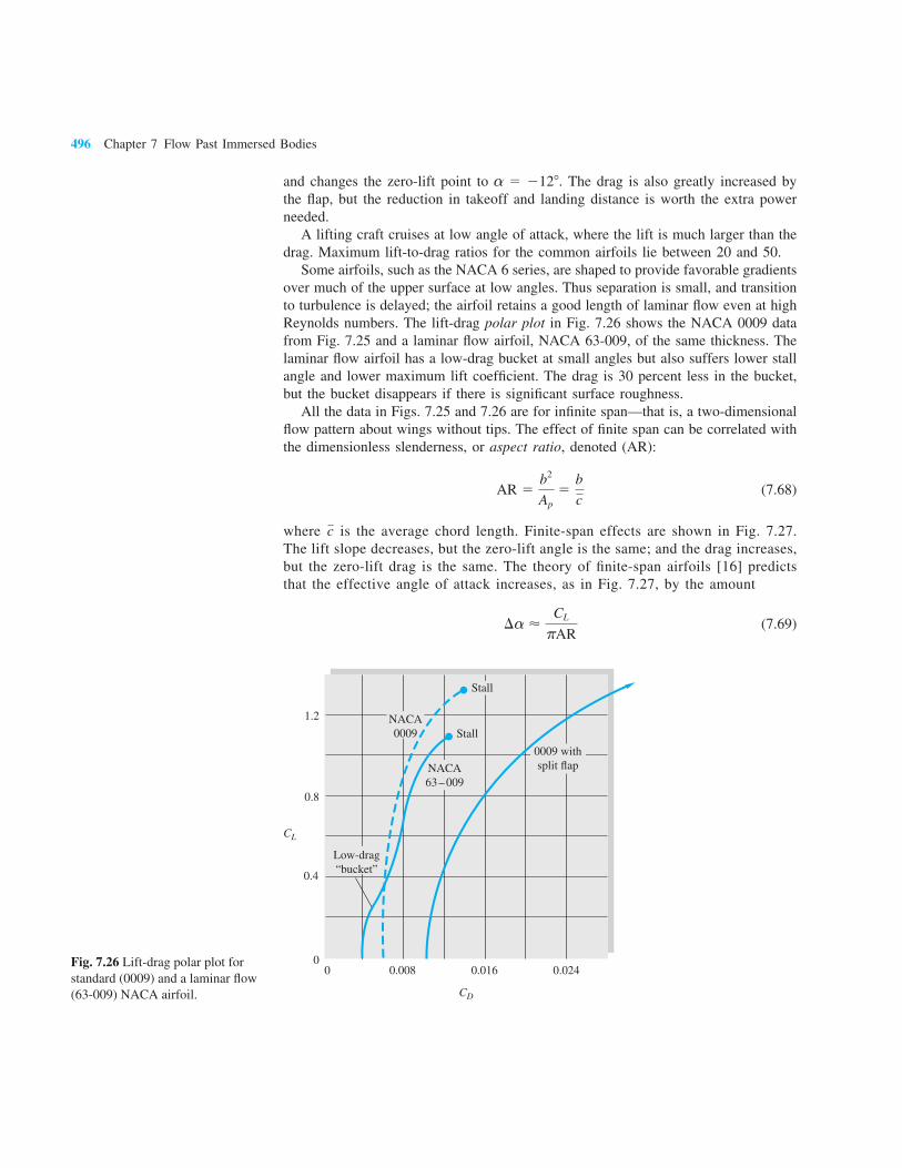
Chapter 7 Flow Past Immersed Bodies

449

Chapter 7 Flow Past

Immersed Bodies

Motivation. This chapter is devoted to “external” fl ows around bodies immersed in a fl uid stream. Such a fl ow will have viscous (shear and no-slip) effects near the body surfaces and in its wake, but will typically be nearly inviscid far from the body. These are unconfi ned boundary layer fl ows. Chapter 6 considered “internal” fl ows confi ned by the walls of a duct. In that case the viscous boundary layers grow from the sidewalls, meet downstream, and fi ll the entire duct. Viscous shear is the dominant effect. For example, the Moody chart of Fig. 6.13 is essentially a correlation of wall shear stress for long ducts of constant cross section. External fl ows are unconfi ned, free to expand no matter how thick the viscous layers grow. Although boundary layer theory (Sec. 7.3) and computational fl uid dynamics (CFD) [4] are helpful in understanding external fl ows, complex body geometries usually require experimental data on the forces and moments caused by the fl ow. Such immersed-body fl ows are commonly encountered in engineering studies: aerodynamics (airplanes, rockets, projectiles), hydrodynamics (ships, submarines, torpedos), transportation (automobiles, trucks, cycles), wind engineering (buildings, bridges, water towers, wind turbines), and ocean engineering (buoys, breakwaters, pilings, cables, moored instruments). This chapter provides data and analysis to assist in such studies.

7.1 Reynolds Number and Geometry Effects

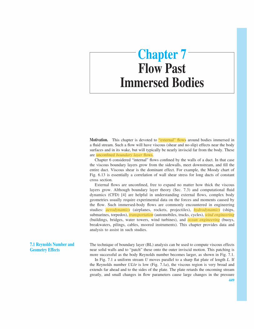
The technique of boundary layer (BL) analysis can be used to compute viscous effects near solid walls and to “patch” these onto the outer inviscid motion. This patching is more successful as the body Reynolds number becomes larger, as shown in Fig. 7.1. In Fig. 7.1 a uniform stream U moves parallel to a sharp fl at plate of length L. If the Reynolds number UL/ν is low (Fig. 7.1a), the viscous region is very broad and extends far ahead and to the sides of the plate. The plate retards the oncoming stream greatly, and small changes in fl ow parameters cause large changes in the pressure

Highlight

Highlight

Highlight

Highlight

Highlight

Highlight

Highlight

450 Chapter 7 Flow Past Immersed Bodies

distribution along the plate. Thus, although in principle it should be possible to patch the viscous and inviscid layers in a mathematical analysis, their interaction is strong and nonlinear [1 to 3]. There is no existing simple theory for external fl ow analysis at Reynolds numbers from 1 to about 1000. Such thick-shear-layer fl ows are typically studied by experiment or by numerical modeling of the fl ow fi eld on a computer [4]. A high-Reynolds-number fl ow (Fig. 7.1b) is much more amenable to boundary layer patching, as fi rst pointed out by Prandtl in 1904. The viscous layers, either laminar or turbulent, are very thin, thinner even than the drawing shows. We defi ne the boundary layer thickness δ as the locus of points where the velocity u parallel to the plate reaches 99 percent of the external velocity U. As we shall see in Sec. 7.4, the accepted formulas for fl at-plate fl ow, and their approximate ranges, are

Large viscousdisplacement

effect

ReL = 10

U

x

L

Viscousregion

Inviscid regionU

U

u < U

u = 0.99Uδ ≈ L

x

U

U

u < UViscous

Inviscid region

δ L

Laminar BL

Turbulent BL

Smalldisplacement

effect

ReL = 107

U

(a)

(b)

Fig. 7.1 Comparison of fl ow past a sharp fl at plate at low and high Reynolds numbers: (a) laminar, low-Re fl ow; (b) high-Re fl ow.

δ

x< μ 5.0

Rex1/2 laminar 103 , Rex , 106

0.16

Rex1/7 turbulent 106 , Rex

(7.1a)

(7.1 b )

Highlight

Highlight

Highlight

7.1 Reynolds Number and Geometry Effects 451

where Rex 5 Ux/ν is called the local Reynolds number of the fl ow along the plate surface. The turbulent fl ow formula applies for Rex greater than approximately 106. Some computed values from Eq. (7.1) are

Rex 104 105 106 107 108

(δ/x)lam 0.050 0.016 0.005

(δ/x)turb 0.022 0.016 0.011

The blanks indicate that the formula is not applicable. In all cases these boundary layers are so thin that their displacement effect on the outer inviscid layer is negligible. Thus the pressure distribution along the plate can be computed from inviscid theory as if the boundary layer were not even there. This external pres-sure fi eld then “drives” the boundary layer fl ow, acting as a forcing function in the momentum equation along the surface. We shall explain this boundary layer theory in Secs. 7.4 and 7.5. For slender bodies, such as plates and airfoils parallel to the oncoming stream, we conclude that this assumption of negligible interaction between the boundary layer and the outer pressure distribution is an excellent approximation. For a blunt-body fl ow, however, even at very high Reynolds numbers, there is a discrepancy in the viscous–inviscid patching concept. Figure 7.2 shows two

(a)

(b)

Thin frontboundary layer

Beautifully behavedbut mythically thin

boundary layerand wake

Outer stream grosslyperturbed by broad flow

separation and wake

Red = 105

Red = 105

Fig. 7.2 Illustration of the strong interaction between viscous and inviscid regions in the rear of blunt-body fl ow: (a) idealized and defi nitely false picture of blunt-body fl ow; (b) actual picture of blunt-body fl ow.

Highlight

Highlight

Highlight

Highlight

Highlight

Highlight

Highlight

Highlight


sketches of fl ow past a two- or three-dimensional blunt body. In the ideal ized sketch (7.2a), there is a thin fi lm of boundary layer about the body and a narrow sheet of viscous wake in the rear. The patching theory would be glorious for this picture, but it is false. In the actual fl ow (Fig. 7.2b), the boundary layer is thin on the front, or windward, side of the body, where the pressure decreases along the surface (favorable pressure gradient). But in the rear the boundary layer encounters increasing pressure (adverse pressure gradient) and breaks off, or sepa-rates, into a broad, pulsating wake. (See Fig. 5.2a for a photograph of a specifi c example.) The mainstream is defl ected by this wake, so that the external fl ow is quite different from the prediction from inviscid theory with the addition of a thin boundary layer. The theory of strong interaction between blunt-body viscous and inviscid layers is not well developed. Flows like that of Fig. 7.2b are normally studied experimentally or with CFD [4]. Reference 5 is an example of efforts to improve the theory of sepa-rated fl ows. Reference 6 is another textbook devoted to separated fl ow.

EXAMPLE 7.1

A long, thin, fl at plate is placed parallel to a 20-ft/s stream of water at 688F. At what distance x from the leading edge will the boundary layer thickness be 1 in?

Solution

• Assumptions: Flat-plate fl ow, with Eqs. (7.1) applying in their appropriate ranges.• Approach: Guess laminar fl ow fi rst. If contradictory, try turbulent fl ow.• Property values: From Table A.1 for water at 688F, ν < 1.082 E-5 ft2/s.• Solution step 1: With δ 5 1 in 5 1/12 ft, try laminar fl ow, Eq. (7.1a):

δ

x0 lam 5

5

(Ux/ν)1/2 or 1/12 ft

x5

53 (20 ft/s)x/ (1.082 E-5 ft2/s) 41/2

Solve for x < 513 ft

Pretty long plate! This does not sound right. Check the local Reynolds number:

Rex 5Ux

ν5

(20 ft/s) (513 ft)

1.082 E-5 ft2/s5 9.5 E8 (!)

This is impossible, since laminar boundary layer fl ow only persists up to about 106 (or, with special care to avoid disturbances, up to 3 3 106).

• Solution step 2: Try turbulent fl ow, Eq. (7.1b):

δ

x5

0.16

(Ux/ν)1/7 or 1/12 ft

x5

0.163 (20 ft/s)x/ (1.082 E-5 ft2/s) 41/7

Solve for x < 5.17 ft Ans.

Check Rex 5 (20 ft/s)(5.17 ft)/(1.082 E-5 ft2/s) 5 9.6 E6 . 106. OK, turbulent fl ow.• Comments: The fl ow is turbulent, and the inherent ambiguity of the theory is

resolved.

Highlight

Highlight

Highlight

Highlight

7.2 Momentum Integral Estimates 453

7.2 Momentum Integral Estimates

When we derived the momentum integral relation, Eq. (3.37), and applied it to a fl at-plate boundary layer in Example 3.11, we promised to consider it further in Chap. 7. Well, here we are! Let us review the problem, using Fig. 7.3. A shear layer of unknown thickness grows along the sharp fl at plate in Fig. 7.3. The no-slip wall condition retards the fl ow, making it into a rounded profi le u(x, y), which merges into the external velocity U 5 constant at a “thickness” y 5 δ(x). By utilizing the control volume of Fig. 3.11, we found (without making any assumptions about laminar versus turbulent fl ow) in Example 3.11 that the drag force on the plate is given by the following momentum integral across the exit plane:

D(x) 5 ρb#δ(x)

0

u(U 2 u) dy (7.2)

where b is the plate width into the paper and the integration is carried out along a vertical plane x 5 constant. You should review the momentum integral relation (3.37) and its use in Example 3.11.

Kármán’s Analysis of the Flat Plate

Equation (7.2) was derived in 1921 by Kármán [7], who wrote it in the convenient form of the m o mentum thickness θ :

D(x) 5 ρbU2θ θ 5#δ

0

u

U a1 2

u

Ub dy (7.3)

Momentum thickness is thus a measure of total plate drag. Kármán then noted that the drag also equals the integrated wall shear stress along the plate:

D(x) 5 b#x

0

τw(x) dx

or dD

dx5 bτw (7.4)

Meanwhile, the derivative of Eq. (7.3), with U 5 constant, is

dD

dx5 ρbU2

dθ

dx

x

y

U

x = 0

p = pa

U

w(x)

x = L

u(x, y)

U

(x)δ

τ

Fig. 7.3 Growth of a boundary layer on a fl at plate. The thickness is exaggerated.

Highlight

Highlight

Highlight

Highlight

Highlight

Highlight


By comparing this with Eq. (7.4) Kármán arrived at what is now called the momentum integral relation for fl at-plate boundary layer fl ow:

τw 5 ρU2 dθ

dx (7.5)

It is valid for either laminar or turbulent fl at-plate fl ow. To get a numerical result for laminar fl ow, Kármán assumed that the velocity profi les had an approximately parabolic shape

u(x, y) < U a2y

δ2

y2

δ2b 0 # y # δ(x) (7.6)

which makes it possible to estimate both momentum thickness and wall shear:

θ 5 #δ

0 a2y

δ2

y2

δ2b a1 22y

δ1

y2

δ2b dy <2

15δ

τw 5 μ0u

0y`y50

<2μU

δ (7.7)

By substituting (7.7) into (7.5) and rearranging, we obtain

δ dδ < 15 ν

U dx (7.8)

where ν 5 μ/ρ. We can integrate from 0 to x, assuming that δ 5 0 at x 5 0, the leading edge:

1

2 δ2 5

15νx

U

or δ

x< 5.5 a ν

Uxb1/2

55.5

Rex1/2 (7.9)

This is the desired thickness estimate. It is all approximate, of course, part of Kármán’s momentum integral theory [7], but it is startlingly accurate, being only 10 percent higher than the known accepted solution for laminar fl at-plate fl ow, which we gave as Eq. (7.1a). By combining Eqs. (7.9) and (7.7) we also obtain a shear stress estimate along the plate:

cf 52τw

ρU2 < a 815

Rexb1/2

50.73

Rex1/2 (7.10)

Again this estimate, in spite of the crudeness of the profi le assumption [Eq. (7.6)] is only 10 percent higher than the known exact laminar-plate-fl ow solution cf 5 0.664/Rex

1/2, treated in Sec. 7.4. The dimensionless quantity cf, called the skin friction coeffi cient, is analogous to the friction factor f in ducts. A boundary layer can be judged as “thin” if, say, the ratio δ/x is less than about 0.1. This occurs at δ/x 5 0.1 5 5.0/Rex

1/2 or at Rex 5 2500. For Rex less than 2500 we can estimate that boundary layer theory fails because the thick layer has a signifi cant effect on the outer inviscid fl ow. The upper limit on Rex for laminar fl ow

Highlight

Highlight

Highlight

Highlight

Highlight

7.2 Momentum Integral Estimates 455

is about 3 3 106, where measurements on a smooth fl at plate [8] show that the fl ow undergoes transition to a turbulent boundary layer. From 3 3 106 upward the turbulent Reynolds number may be arbitrarily large, and a practical limit at present is 5 3 1010 for oil supertankers.

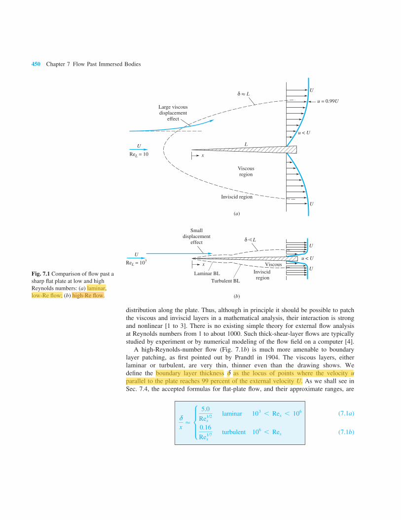
Displacement Thickness Another interesting effect of a boundary layer is its small but fi nite displacement of the outer streamlines. As shown in Fig. 7.4, outer streamlines must defl ect outward a distance δ*(x) to satisfy conservation of mass between the inlet and outlet:

#h

0

ρUb dy 5 #δ

0

ρub dy δ 5 h 1 δ* (7.11)

The quantity δ* is called the displacement thickness of the boundary layer. To relate it to u(y), cancel ρ and b from Eq. (7.11), evaluate the left integral, and slyly add and subtract U from the right integrand:

Uh 5 #δ

0

(U 1 u 2 U) dy 5 U(h 1 δ*) 1 #δ

0

(u 2 U) dy

or δ* 5 #δ

0

a1 2u

Ub dy (7.12)

Thus the ratio of δ*/δ varies only with the dimensionless velocity profi le shape u/U. Introducing our profi le approximation (7.6) into (7.12), we obtain by integration this approximate result:

δ* <1

3 δ

δ*x

<1.83

Rex1/2 (7.13)

These estimates are only 6 percent away from the exact solutions for laminar fl at-plate fl ow given in Sec. 7.4: δ* 5 0.344δ 5 1.721x/Rex

1/2. Since δ* is much smaller than x for large Rex and the outer streamline slope V/U is proportional to δ*, we conclude that the velocity normal to the wall is much smaller than the velocity parallel to the wall. This is a key assumption in boundary layer theory (Sec. 7.3). We also conclude from the success of these simple parabolic estimates that Kármán’s momentum integral theory is effective and useful. Many details of this theory are given in Refs. 1 to 3.

yU U

Simulatedeffect

0

y = h

x

Outer streamline

y = h + δ

U

uδ *

h

h

*

Fig. 7.4 Displacement effect of a boundary layer.

Highlight

Highlight

Highlight

Highlight

Highlight


EXAMPLE 7.2

Are low-speed, small-scale air and water boundary layers really thin? Consider fl ow at U 5 1 ft/s past a fl at plate 1 ft long. Compute the boundary layer thickness at the trailing edge for (a) air and (b) water at 688F.

Solution

Part (a) From Table A.2, νair < 1.61 E-4 ft2/s. The trailing-edge Reynolds number thus is

ReL 5UL

ν5

(1 ft/s) (1 ft)

1.61 E-4 ft2/s5 6200

Since this is less than 106, the fl ow is presumed laminar, and since it is greater than 2500, the boundary layer is reasonably thin. From Eq. (7.1a), the predicted laminar thickness is

δ

x5

5.0

162005 0.0634

or, at x 5 1 ft, δ 5 0.0634 ft < 0.76 in Ans. (a)

Part (b) From Table A.1, νwater < 1.08 E-5 ft2/s. The trailing-edge Reynolds number is

ReL 5(1 ft/s) (1 ft)

1.08 E-5 ft2/s< 92,600

This again satisfi es the laminar and thinness conditions. The boundary layer thickness is

δ

x<

5.0

192,6005 0.0164

or, at x 5 1 ft, δ 5 0.0164 ft < 0.20 in Ans. (b)

Thus, even at such low velocities and short lengths, both airfl ows and water fl ows satisfy the boundary layer approximations.

7.3 The Boundary Layer Equations

In Chaps. 4 and 6 we learned that there are several dozen known analytical laminar fl ow solutions [1 to 3]. None are for external fl ow around immersed bodies, although this is one of the primary applications of fl uid mechanics. No exact solutions are known for turbulent fl ow, whose analysis typically uses empirical modeling laws to relate time-mean variables. There are presently three techniques used to study external fl ows: (1) numerical (computer) solutions, (2) experimentation, and (3) boundary layer theory. Computational fluid dynamics is now well developed and described in advanced texts such as that by Anderson [4]. Thousands of computer solutions and models have been published; execution times, mesh sizes, and graphical presentations are improving each year. Both laminar and turbulent flow solutions have been published, and turbulence modeling is a current research topic [9]. Except for a brief discussion of computer analysis in Chap. 8, the topic of CFD is beyond our scope here.

7.3 The Boundary Layer Equations 457

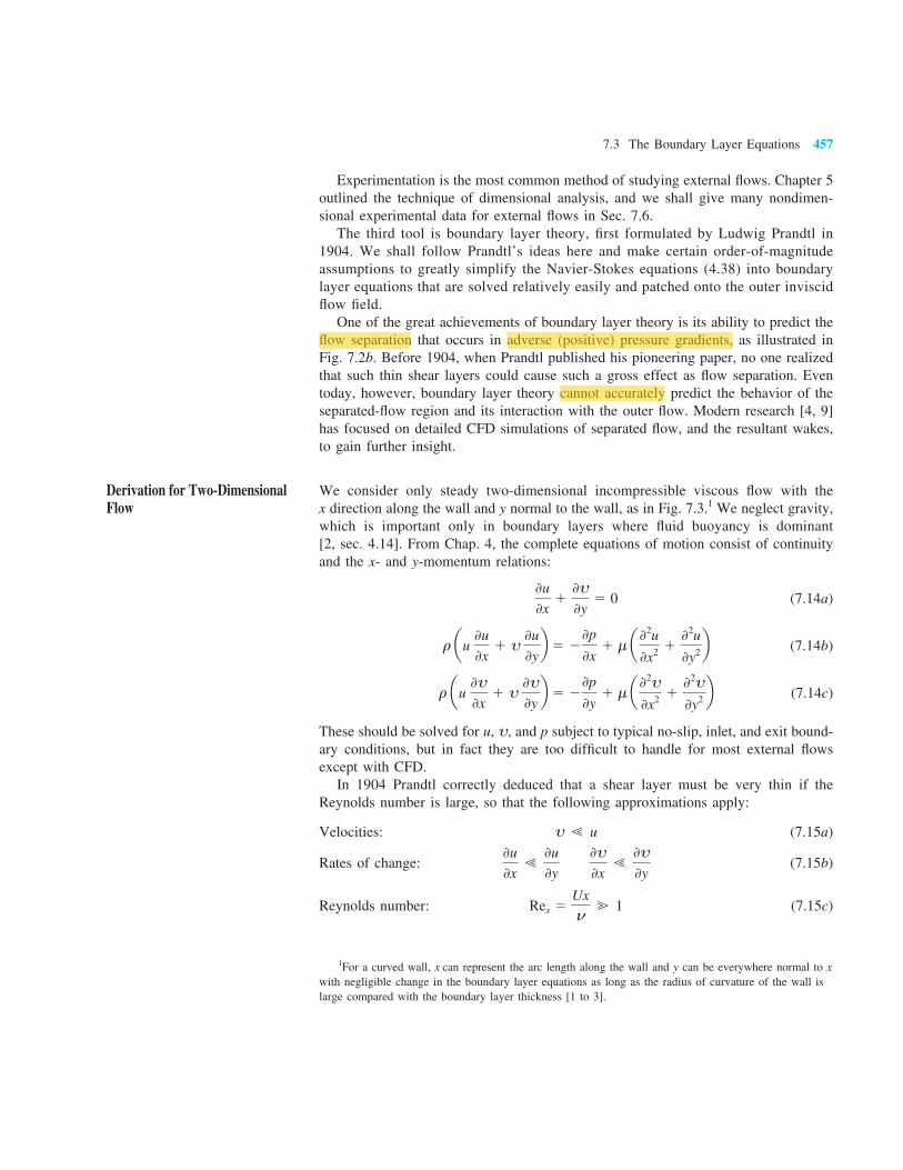
Experimentation is the most common method of studying external fl ows. Chapter 5 outlined the technique of dimensional analysis, and we shall give many nondimen-sional experimental data for external fl ows in Sec. 7.6. The third tool is boundary layer theory, fi rst formulated by Ludwig Prandtl in 1904. We shall follow Prandtl’s ideas here and make certain order-of-magnitude assumptions to greatly simplify the Navier-Stokes equations (4.38) into boundary layer equations that are solved relatively easily and patched onto the outer inviscid fl ow fi eld. One of the great achievements of boundary layer theory is its ability to predict the fl ow separation that occurs in adverse (positive) pressure gradients, as illustrated in Fig. 7.2b. Before 1904, when Prandtl published his pioneering paper, no one realized that such thin shear layers could cause such a gross effect as fl ow separation. Even today, however, boundary layer theory cannot accurately predict the behavior of the separated-fl ow region and its interaction with the outer fl ow. Modern research [4, 9] has focused on detailed CFD simulations of separated fl ow, and the resultant wakes, to gain further insight.

Derivation for Two-Dimensional Flow

We consider only steady two-dimensional incompressible viscous fl ow with the x direction along the wall and y normal to the wall, as in Fig. 7.3.1 We neglect gravity, which is important only in boundary layers where fl uid buoyancy is dominant [2, sec. 4.14]. From Chap. 4, the complete equations of motion consist of continuity and the x- and y-momentum relations:

0u

0x1

0υ0y

5 0 (7.14a)

ρ au 0u

0x1 υ

0u

0yb 5 2

0p

0x1 μ a 02u

0x2 102u

0y2b (7.14b)

ρ au 0υ0x

1 υ 0υ0yb 5 2

0p

0y1 μ a 02υ

0x2 102υ

0y2 b (7.14c)

These should be solved for u, υ, and p subject to typical no-slip, inlet, and exit bound-ary conditions, but in fact they are too diffi cult to handle for most external fl ows except with CFD. In 1904 Prandtl correctly deduced that a shear layer must be very thin if the Reynolds number is large, so that the following approximations apply:

Velocities: υ ! u (7.15a)

Rates of change: 0u

0x!

0u

0y

0υ0x

!0υ0y

(7.15b)

Reynolds number: Rex 5Ux

ν@ 1 (7.15c)

1For a curved wall, x can represent the arc length along the wall and y can be everywhere normal to x

with negligible change in the boundary layer equations as long as the radius of curvature of the wall is large compared with the boundary layer thickness [1 to 3].

Highlight

Highlight

Highlight


Our discussion of displacement thickness in the previous section was intended to justify these assumptions. Applying these approximations to Eq. (7.14c) results in a powerful simplifi cation:

ρ au0υ0x

b 1 ρ aυ

0υ0y

b 5 20p

0y1 μ a 02υ

0x2 b 1 μ a 02υ

0y2 b small small very small small

0p

0y< 0 or p < p(x) only (7.16)

In other words, the y-momentum equation can be neglected entirely, and the pressure varies only along the boundary layer, not through it. The pressure gradient term in Eq. (7.14b) is assumed to be known in advance from Bernoulli’s equation applied to the outer inviscid fl ow:

0p

0x5

dp

dx5 2ρU

dU

dx (7.17)

Presumably we have already made the inviscid analysis and know the distribution of U(x) along the wall (Chap. 8). Meanwhile, one term in Eq. (7.14b) is negligible due to Eqs. (7.15):

02u

0x2 !02u

0y2 (7.18)

However, neither term in the continuity relation (7.14a) can be neglected—another warning that continuity is always a vital part of any fl uid fl ow analysis. The net result is that the three full equations of motion (7.14) are reduced to Prandtl’s two boundary layer equations for two-dimensional incompressible fl ow:

Continuity: 0u

0x1

0υ0y

5 0 (7.19a)

Momentum along wall: u 0u

0x1 υ

0u

0y< U

dU

dx1

1ρ

0τ0y

(7.19b)

where τ 5 μ μ 0u

0ylaminar flow

μ 0u

0y2 ρu¿υ¿ turbulent flow

These are to be solved for u(x, y) and υ(x, y), with U(x) assumed to be a known function from the outer inviscid fl ow analysis. There are two boundary conditions on u and one on υ:

At y 5 0 (wall): u 5 υ 5 0 (no slip) (7.20a)

As y 5 δ(x) (other stream): u 5 U(x) (patching) (7.20b)

Unlike the Navier-Stokes equations (7.14), which are mathematically elliptic and must be solved simultaneously over the entire fl ow fi eld, the boundary layer equations (7.19)

Highlight

Highlight

Highlight

Highlight

Highlight

Highlight

7.4 The Flat-Plate Boundary Layer 459

are mathematically parabolic and are solved by beginning at the leading edge and marching downstream as far as you like, stopping at the separation point or earlier if you prefer.2

The boundary layer equations have been solved for scores of interesting cases of internal and external fl ow for both laminar and turbulent fl ow, utilizing the inviscid distribution U(x) appropriate to each fl ow. Full details of boundary layer theory and results and comparison with experiment are given in Refs. 1 to 3. Here we shall confi ne ourselves primarily to fl at-plate solutions (Sec. 7.4).

7.4 The Flat-Plate Boundary Layer

The classic and most often used solution of boundary layer theory is for fl at-plate fl ow, as in Fig. 7.3, which can represent either laminar or turbulent fl ow.

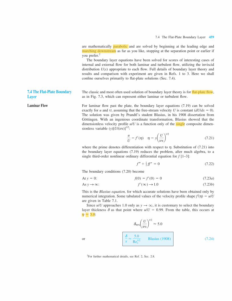
Laminar Flow For laminar fl ow past the plate, the boundary layer equations (7.19) can be solved exactly for u and υ, assuming that the free-stream velocity U is constant (dU/dx 5 0). The solution was given by Prandtl’s student Blasius, in his 1908 dissertation from Göttingen. With an ingenious coordinate transformation, Blasius showed that the dimensionless velocity profi le u/U is a function only of the single composite dimen-sionless variable (y)[U/(νx)]1/2:

u

U5 f ¿ (η) η 5 y a U

νxb1/2

(7.21)

where the prime denotes differentiation with respect to η. Substitution of (7.21) into the boundary layer equations (7.19) reduces the problem, after much algebra, to a single third-order nonlinear ordinary differential equation for f [1–3]:

f Ô 1 12 ff – 5 0 (7.22)

The boundary conditions (7.20) become

At y 5 0: f(0) 5 f ¿ (0) 5 0 (7.23a)

As y S ∞: f ¿ (∞ ) S 1.0 (7.23b)

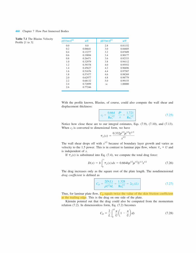
This is the Blasius equation, for which accurate solutions have been obtained only by numerical integration. Some tabulated values of the velocity profi le shape f '(η) 5 u/U are given in Table 7.1. Since u/U approaches 1.0 only as y → q , it is customary to select the boundary layer thickness δ as that point where u/U 5 0.99. From the table, this occurs at η < 5.0:

δ99%a U

νxb1/2

< 5.0

or δ

x<

5.0

Re1/2x

Blasius (1908) (7.24)

2For further mathematical details, see Ref. 2, Sec. 2.8.

Highlight

Highlight

Highlight

Highlight

Highlight


Table 7.1 The Blasius Velocity Profi le [1 to 3]

y [ U /( ν x )] 1/2 u/U y [ U /( ν x )] 1/2 u / U

0.0 0.0 2.8 0.81152 0.2 0.06641 3.0 0.84605 0.4 0.13277 3.2 0.87609 0.6 0.19894 3.4 0.90177 0.8 0.26471 3.6 0.92333 1.0 0.32979 3.8 0.94112 1.2 0.39378 4.0 0.95552 1.4 0.45627 4.2 0.96696 1.6 0.51676 4.4 0.97587 1.8 0.57477 4.6 0.98269 2.0 0.62977 4.8 0.98779 2.2 0.68132 5.0 0.99155 2.4 0.72899 q 1.00000 2.6 0.77246

With the profi le known, Blasius, of course, could also compute the wall shear and displacement thickness:

cf 50.664

Re1/2x

δ*x

51.721

Re1/2x

(7.25)

Notice how close these are to our integral estimates, Eqs. (7.9), (7.10), and (7.13). When cf is converted to dimensional form, we have

τw(x) 50.332ρ1/2μ1/2U1.5

x1/2

The wall shear drops off with x1/2 because of boundary layer growth and varies as velocity to the 1.5 power. This is in contrast to laminar pipe fl ow, where τw ~ U and is independent of x. If τw(x) is substituted into Eq. (7.4), we compute the total drag force:

D(x) 5 b#x

0

τw(x) dx 5 0.664bρ1/2μ1/2U1.5x1/2 (7.26)

The drag increases only as the square root of the plate length. The nondimensional drag coeffi cient is defi ned as

CD 52D(L)

ρU2bL5

1.328

Re1/2L

5 2cf (L) (7.27)

Thus, for laminar plate fl ow, C D equals twice the value of the skin fri c tion coeffi cient at the trailing edge. This is the drag on one side of the plate. Kármán pointed out that the drag could also be computed from the momentum relation (7.2). In dimensionless form, Eq. (7.2) becomes

CD 52

L #δ

0

u

U a1 2

u

Ub dy (7.28)

Highlight


This can be rewritten in terms of the momentum thickness at the trailing edge:

CD 52θ(L)

L (7.29)

Computation of θ from the profi le u/U or from CD gives

θ

x5

0.664

Re1/2x

laminar flat plate (7.30)

Since δ is so ill defi ned, the momentum thickness, being defi nite, is often used to correlate data taken for a variety of boundary layers under differing conditions. The ratio of displacement to momentum thickness, called the dimensionless-profi le shape factor, is also useful in integral theories. For laminar fl at-plate fl ow

H 5δ*

θ5

1.721

0.6645 2.59 (7.31)

A large shape factor then implies that boundary layer separation is about to occur. If we plot the Blasius velocity profi le from Table 7.1 in the form of u/U versus y/δ, we can see why the simple integral theory guess, Eq. (7.6), was such a great success. This is done in Fig. 7.5. The simple parabolic approximation is not far from the true Blasius profi le; hence its momentum thickness is within 10 percent of the true value. Also shown in Fig. 7.5 are three typical turbulent fl at-plate velocity pro-fi les. Notice how strikingly different in shape they are from the laminar profi les.

1.0

0.8

0.6

0.4

0.2

00.2 0.4 0.6 0.8 1.0

uU

y

δ

Turbulent

105 = Rex106

107

Seventhroot profile,Eq. (7.39)

Exact Blasius profilefor all laminar Rex

(Table 7.1)

Parabolicapproximation,

Eq. (7.6)

Fig. 7.5 Comparison of dimensionless laminar and turbulent fl at-plate velocity profi les.


Instead of decreasing parabolically to zero, the turbulent profi les are very fl at and then drop off sharply at the wall. As you might guess, they follow the logarithmic law shape and thus can be analyzed by momentum integral theory if this shape is properly represented.

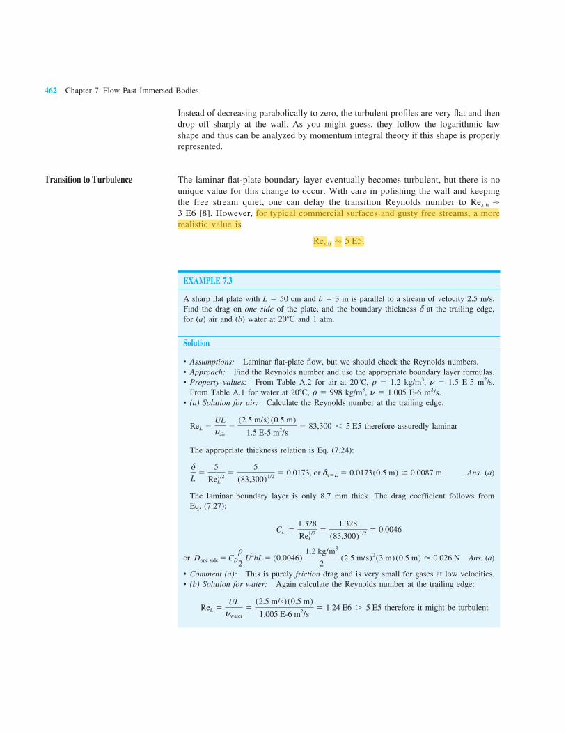
Transition to Turbulence The laminar fl at-plate boundary layer eventually becomes turbulent, but there is no unique value for this change to occur. With care in polishing the wall and keeping the free stream quiet, one can delay the transition Reynolds number to Rex,tr < 3 E6 [8]. However, for typical commercial surfaces and gusty free streams, a more realistic value is

Rex,tr < 5 E5.

EXAMPLE 7.3

A sharp fl at plate with L 5 50 cm and b 5 3 m is parallel to a stream of velocity 2.5 m/s. Find the drag on one side of the plate, and the boundary thickness δ at the trailing edge, for (a) air and (b) water at 208C and 1 atm.

Solution

• Assumptions: Laminar fl at-plate fl ow, but we should check the Reynolds numbers.• Approach: Find the Reynolds number and use the appropriate boundary layer formulas.• Property values: From Table A.2 for air at 208C, ρ 5 1.2 kg/m3, ν 5 1.5 E-5 m2/s.

From Table A.1 for water at 208C, ρ 5 998 kg/m3, ν 5 1.005 E-6 m2/s.• (a) Solution for air: Calculate the Reynolds number at the trailing edge:

ReL 5UL

νair5

(2.5 m/s)(0.5 m)

1.5 E-5 m2/s5 83,300 , 5 E5 therefore assuredly laminar

The appropriate thickness relation is Eq. (7.24):

δ

L5

5

Re1/2L

55

(83,300)1/2 5 0.0173, or δx5L 5 0.0173(0.5 m) > 0.0087 m Ans. (a)

The laminar boundary layer is only 8.7 mm thick. The drag coeffi cient follows from Eq. (7.27):

CD 51.328

Re1/2L

51.328

(83,300)1/2 5 0.0046

or Done side 5 CD

ρ

2 U2bL 5 (0.0046)

1.2 kg/m3

2 (2.5 m/s)2(3 m)(0.5 m) < 0.026 N Ans. (a)

• Comment (a): This is purely friction drag and is very small for gases at low velocities.• (b) Solution for water: Again calculate the Reynolds number at the trailing edge:

ReL 5UL

νwater5

(2.5 m/s)(0.5 m)

1.005 E-6 m2/s5 1.24 E6 . 5 E5 therefore it might be turbulent

Highlight

Highlight


This is a quandary. If the plate is rough or encounters disturbances, the fl ow at the trailing edge will be turbulent. Let us assume a smooth, undisturbed plate, which will remain laminar. Then again the appropriate thickness relation is Eq. (7.24):

δ

L5

5

Re1/2L

55

(1.24 E6)1/2 5 0.00448 or δx5L 5 0.00448(0.5 m) > 0.0022 m Ans. (b)

This is four times thinner than the air result in part (a), due to the high laminar Reynolds number. Again the drag coeffi cient follows from Eq. (7.27):

CD 51.328

Re1/2L

51.328

(1.24 E6)1/2 5 0.0012

or Done side 5 CD

ρ

2 U2bL 5 (0.0012)

998 kg/m3

2 (2.5 m/s)2(3 m)(0.5 m) < 5.6 N Ans. (b)

• Comment (b): The drag is 215 times larger for water, although CD is lower, refl ecting that water is 56 times more viscous and 830 times denser than air. From Eq. (7.26), for the same U and x, the water drag should be (56)1/2(830)1/2 < 215 times higher. Note: If transition to turbulence had occurred at Rex 5 5 E5 (at about x 5 20 cm), the drag would be about 2.5 times higher, and the trailing edge thickness about four times higher than for fully laminar fl ow.

Turbulent Flow There is no exact theory for turbulent fl at-plate fl ow, although there are many elegant computer solutions of the boundary layer equations using various empirical models for the turbulent eddy viscosity [9]. The most widely accepted result is simply an integral analysis similar to our study of the laminar profi le approximation (7.6). We begin with Eq. (7.5), which is valid for laminar or turbulent fl ow. We write it here for convenient reference:

τw(x) 5 ρU2

dθ

dx (7.32)

From the defi nition of cf, Eq. (7.10), this can be rewritten as

cf 5 2dθ

dx (7.33)

Now recall from Fig. 7.5 that the turbulent profi les are nowhere near parabolic. Going back to Fig. 6.10, we see that fl at-plate fl ow is very nearly logarithmic, with a slight outer wake and a thin viscous sublayer. Therefore, just as in turbulent pipe fl ow, we assume that the logarithmic law (6.28) holds all the way across the boundary layer

u

u*<

1κ

ln yu*

ν1 B u* 5 aτw

ρb1/2

(7.34)

with, as usual, κ 5 0.41 and B 5 5.0. At the outer edge of the boundary layer, y 5 δ and u 5 U, and Eq. (7.34) becomes

U

u*5

1κ

ln δu*ν

1 B (7.35)

Highlight


But the defi nition of the skin friction coeffi cient, Eq. (7.10), is such that the following identities hold:

U

u*; a 2

cfb1/2

δu*ν

; Reδ acf

2b1/2

(7.36)

Therefore, Eq. (7.35) is a skin friction law for turbulent fl at-plate fl ow: a 2cfb1/2

< 2.44 ln cReδ acf

2b1/2 d 1 5.0 (7.37)

It is a complicated law, but we can at least solve for a few values and list them:

Reδ 104 105 106 107

cf 0.00493 0.00315 0.00217 0.00158

Following a suggestion of Prandtl, we can forget the complex log friction law (7.37) and simply fi t the numbers in the table to a power-law approximation:

cf < 0.02 Re21/6δ (7.38)

This we shall use as the left-hand side of Eq. (7.33). For the right-hand side, we need an estimate for θ(x) in terms of δ(x). If we use the logarithmic law profi le (7.34), we shall be up to our hips in logarithmic integrations for the momentum thickness. Instead we follow another suggestion of Prandtl, who pointed out that the turbulent profi les in Fig. 7.5 can be approximated by a one-seventh-power law:a u

Ub

turb< a y

δb1/7

(7.39)

This is shown as a dashed line in Fig. 7.5. It is an excellent fi t to the low-Reynolds-number turbulent data, which were all that were available to Prandtl at the time. With this simple approximation, the momentum thickness (7.28) can easily be evaluated:

θ < #δ

0

a y

δb1/7 c1 2 a y

δb1/7 ddy 5

7

72 δ (7.40)

We accept this result and substitute Eqs. (7.38) and (7.40) into Kármán’s momentum law (7.33):

cf 5 0.02 Reδ21/6 5 2

d

dx a 7

72 δb

or Reδ21/6 5 9.72

dδ

dx5 9.72

d(Reδ)

d(Rex) (7.41)

Separate the variables and integrate, assuming δ 5 0 at x 5 0:

Reδ < 0.16 Rex6/7 or

δ

x<

0.16

Rex1/7 (7.42)

Thus the thickness of a turbulent boundary layer increases as x6/7, far more rapidly than the laminar increase x1/2. Equation (7.42) is the solution to the problem, because

Highlight

Highlight

Highlight

Highlight

Highlight

Highlight

Highlight


all other parameters are now available. For example, combining Eqs. (7.42) and (7.38), we obtain the friction variation

cf <0.027

Rex1/7 (7.43)

Writing this out in dimensional form, we have

τw,turb <0.0135μ1/7ρ6/7U13/7

x1/7 (7.44)

Turbulent plate friction drops slowly with x, increases nearly as ρ and U2, and is rather insensitive to viscosity. We can evaluate the drag coeffi cient by integrating the wall friction:

D 5 #L

0

τwb dx

or CD 52D

ρU2 bL5 #

1

0

cf d a x

Lb

CD 50.031

ReL1/7 5

7

6 cf (L) (7.45)

Then CD is only 16 percent greater than the trailing-edge skin friction coeffi cient [compare with Eq. (7.27) for laminar fl ow]. The displacement thickness can be estimated from the one-seventh-power law and Eq. (7.12):

δ* < #δ

0

c1 2 ay

δb1/7 ddy 5

1

8 δ (7.46)

The turbulent fl at-plate shape factor is approximately

H 5δ*

θ5

187

72

5 1.3 (7.47)

These are the basic results of turbulent fl at-plate theory. Figure 7.6 shows fl at-plate drag coeffi cients for both laminar and turbulent fl ow conditions. The smooth-wall relations (7.27) and (7.45) are shown, along with the effect of wall roughness, which is quite strong. The proper roughness parameter here is x/ε or L/ε, by analogy with the pipe parameter ε/d. In the fully rough regime, CD is independent of the Reynolds number, so that the drag varies exactly as U2 and is independent of μ. Reference 2 presents a theory of rough fl at-plate fl ow, and Ref. 1 gives a curve fi t for skin friction and drag in the fully rough regime:

cf < a2.87 1 1.58 log x

εb22.5

(7.48a)

CD < a1.89 1 1.62 log L

εb22.5

(7.48b)

Highlight

Highlight

Highlight

Highlight

Highlight

Highlight


(7.49a)

(7.49b)

Equation (7.48b) is plotted to the right of the dashed line in Fig. 7.6. The fi gure also shows the behavior of the drag coeffi cient in the transition region 5 3 105 , ReL , 8 3 107, where the laminar drag at the leading edge is an appreciable fraction of the total drag. Schlichting [1] su g gests the following curve fi ts for these transition drag curves, depending on the Reynolds number Re trans where transition begins:

CD < μ 0.031

Re1/7L

21440

ReL Retrans 5 5 3 105

0.031

Re1/7L

28700

ReL Retrans 5 3 3 106

EXAMPLE 7.4

A hydrofoil 1.2 ft long and 6 ft wide is placed in a seawater fl ow of 40 ft/s, with ρ 5 1.99 slugs/ft3 and ν 5 0.000011 ft2/s. (a) Estimate the boundary layer thickness at the end of the plate. Estimate the friction drag for (b) turbulent smooth-wall fl ow from the leading

0.014

0.012

0.010

0.008

0.006

0.004

0105 108

ReL

Laminar:Eq. (7.27)

Turbulentsmooth

Eq. (7.45)

Transition

Eq. (7.49)

200

500

1000

2000

104

2 × 104

2 × 105

0.002

106 107 109

CD

5 × 104

L�

= 300

106

Fully roughEq. (7.48b)

5000

Fig. 7.6 Drag coeffi cient of laminar and turbulent boundary layers on smooth and rough fl at plates. This chart is the fl at-plate analog of the Moody diagram of Fig. 6.13.

Highlight


edge, (c) laminar turbulent fl ow with Retrans 5 5 3 105, and (d) turbulent rough-wall fl ow with ε 5 0.0004 ft.

Solution

Part (a) The Reynolds number is

ReL 5UL

ν5

(40 ft/s) (1.2 ft)

0.000011 ft2/s5 4.36 3 106

Thus the trailing-edge fl ow is certainly turbulent. The maximum boundary layer thickness would occur for turbulent fl ow starting at the leading edge. From Eq. (7.42),

δ(L)

L5

0.16

(4.36 3 106)1/7 5 0.018

or δ 5 0.018(1.2 ft) 5 0.0216 ft Ans. (a)

This is 7.5 times thicker than a fully laminar boundary layer at the same Reynolds number.

Part (b) For fully turbulent smooth-wall fl ow, the drag coeffi cient on one side of the plate is, from Eq. (7.45),

CD 50.031

(4.36 3 106)1/7 5 0.00349

Then the drag on both sides of the foil is approximately

D 5 2CD(12 ρU2)bL 5 2(0.00349)(1

2) (1.99)(40)2(6.0)(1.2) 5 80 lbf Ans. (b)

Part (c) With a laminar leading edge and Retrans 5 5 3 105, Eq. (7.49a) applies:

CD 5 0.00349 21440

4.36 3 106 5 0.00316

The drag can be recomputed for this lower drag coeffi cient:

D 5 2CD(12 ρU2)bL 5 72 lbf Ans. (c)

Part (d) Finally, for the rough wall, we calculate

L

ε5

1.2 ft

0.0004 ft5 3000

From Fig. 7.6 at ReL 5 4.36 3 106, this condition is just inside the fully rough regime. Equation (7.48b) applies:

CD 5 (1.89 1 1.62 log 3000)22.5 5 0.00644

and the drag estimate is

D 5 2CD(12 ρU2)bL 5 148 lbf Ans. (d)

This small roughness nearly doubles the drag. It is probable that the total hydrofoil drag is still another factor of 2 larger because of trailing-edge fl ow separation effects.


7.5 Boundary Layers with Pressure Gradient3

The fl at-plate analysis of the previous section should give us a good feeling for the behavior of both laminar and turbulent boundary layers, except for one important effect: fl ow separation. Prandtl showed that separation like that in Fig. 7.2b is caused by excessive momentum loss near the wall in a boundary layer trying to move down-stream against increasing pressure, dp/dx . 0, which is called an adverse pressure gradient. The opposite case of decreasing pressure, dp/dx , 0, is called a favorable gradient, where fl ow separation can never occur. In a typical immersed-body fl ow, such as in Fig. 7.2b, the favorable gradient is on the front of the body and the adverse gradient is in the rear, as discussed in detail in Chap. 8. We can explain fl ow separation with a geometric argument about the second deriv-ative of velocity u at the wall. From the momentum equation (7.19b) at the wall, where u 5 υ 5 0, we obtain

0τ0y

`wall

5 μ

02u

0y2 `wall

5 2ρU dU

dx5

dp

dx

or 02u

0y2 `wall

51μ

dp

dx (7.50)

for either laminar or turbulent fl ow. Thus in an adverse gradient the second deriva-tive of velocity is positive at the wall; yet it must be negative at the outer layer (y 5 δ) to merge smoothly with the mainstream fl ow U(x). It follows that the second derivative must pass through zero somewhere in between, at a point of infl ection, and any boundary layer profi le in an adverse gradient must exhibit a characteristic S shape. Figure 7.7 illustrates the general case. In a favorable gradient (Fig. 7.7a) the profile is very rounded, there is no point of inflection, there can be no separa-tion, and laminar profiles of this type are very resistant to a transition to turbu-lence [1 to 3]. In a zero pressure gradient (Fig. 7.7b), such as a fl at-plate fl ow, the point of infl ec-tion is at the wall itself. There can be no separation, and the fl ow will undergo transi-tion at Rex no greater than about 3 3 106, as discussed earlier. In an adverse gradient (Fig. 7.7c to e), a point of infl ection (PI) occurs in the boundary layer, its distance from the wall increasing with the strength of the adverse gradient. For a weak gradient (Fig. 7.7c) the fl ow does not actually sepa-rate, but it is vulnerable to transition to turbulence at Rex as low as 105 [1, 2]. At a moderate gradient, a critical condition (Fig. 7.7d) is reached where the wall shear is exactly zero (∂u/∂y 5 0). This is defi ned as the separation point (τw 5 0), because any stronger gradient will actually cause backfl ow at the wall (Fig. 7.7e): the boundary layer thickens greatly, and the main fl ow breaks away, or separates, from the wall (Fig. 7.2b). The fl ow profi les of Fig. 7.7 usually occur in sequence as the boundary layer progresses along the wall of a body. For example, in Fig. 7.2a, a favorable gradient occurs on the front of the body, zero pressure gradient occurs just upstream of the shoulder, and an adverse gradient occurs successively as we move around the rear of the body.

3This section may be omitted without loss of continuity.

Highlight

7.5 Boundary Layers with Pressure Gradient 469

A second practical example is the fl ow in a duct consisting of a nozzle, throat, and diffuser, as in Fig. 7.8. The nozzle fl ow is a favorable gradient and never separates, nor does the throat fl ow where the pressure gradient is approximately zero. But the expanding-area diffuser produces low velocity and increasing pres-sure, an adverse gradient. If the diffuser angle is too large, the adverse gradient is excessive, and the boundary layer will separate at one or both walls, with backfl ow,

U

u

PI

(a) Favorablegradient:dUdx

> 0

dp

dx< 0

No separation,PI inside wall

(b) Zerogradient:dUdx

= 0

dp

dx= 0

No separation,PI at wall

PIτw = 0

(c) Weak adversegradient:

dUdx

< 0

dp

dx> 0

No separation,PI in the flow

(d) Critical adversegradient:

Zero slopeat the wall:

Separation

(e) Excessive adversegradient:

Backflowat the wall:

Separatedflow region

U

u

U

u

U

u

U

u

dp

dx> 0

PI

PI

Backflow

Fig. 7.7 Effect of pressure gradient on boundary layer profi les; PI 5 point of infl ection.


increased losses, and poor pressure recovery. In the diffuser literature [10] this condition is called diffuser stall, a term used also in airfoil aerodynamics (Sec. 7.6) to denote airfoil boundary layer separation. Thus the boundary layer behavior explains why a large-angle diffuser has heavy fl ow losses (Fig. 6.23) and poor performance (Fig. 6.28). Presently boundary layer theory can compute only up to the separation point, after which it is invalid. Techniques are now developed for analyzing the strong interaction effects caused by separated fl ows [5, 6].

Laminar Integral Theory4 Both laminar and turbulent theories can be developed from Kármán’s general two-dimensional boundary layer integral relation [2, 7], which extends Eq. (7.33) to vari-able U(x) by integration across the boundary layer:

τw

ρU2 51

2 cf 5

dθ

dx1 (2 1 H)

θ

U dU

dx (7.51)

Nearlyinviscid

core flow

Boundarylayers

U(x)

Profile pointof inflection

Separationpoint

w = 0

x

Dividingstreamline

Backflow

Separation

Nozzle:Decreasing

pressureand area

Increasingvelocity

Favorablegradient

Throat:Constantpressureand area

Velocityconstant

Zerogradient

Diffuser:Increasing pressure

and area

Decreasing velocity

Adverse gradient(boundary layer thickens)

U(x)(x)δ

(x)δ

τ

Fig. 7.8 Boundary layer growth and separation in a nozzle–diffuser confi guration.

4This section may be omitted without loss of continuity.


where θ(x) is the momentum thickness and H(x) 5 δ*(x)/θ(x) is the shape factor. From Eq. (7.17) negative dU/dx is equivalent to positive dp/dx—that is, an adverse gradient. We can integrate Eq. (7.51) to determine θ(x) for a given U(x) if we correlate cf and H with the momentum thickness. This has been done by examining typical veloc-ity profi les of laminar and turbulent boundary layer fl ows for various pressure gradi-ents. Some examples are given in Fig. 7.9, showing that the shape factor H is a good indicator of the pressure gradient. The higher the H, the stronger the adverse gradient, and separation occurs approximately at

H < e3.5 laminar flow

2.4 turbulent flow (7.52)

The laminar profi les (Fig. 7.9a) clearly exhibit the S shape and a point of infl ection with an adverse gradient. But in the turbulent profi les (Fig. 7.9b) the points of infl ec-tion are typically buried deep within the thin viscous sublayer, which can hardly be seen on the scale of the fi gure. There are scores of turbulent theories in the literature, but they are all compli-cated algebraically and will be omitted here. The reader is referred to advanced texts [1–3, 9].

1.0

0.8

0.6

0.2

0.2 0.4 0.6 0.8 1.0

Favorablegradients:

uU

y

δ

(a)

Points ofinflection(adverse

gradients)

3.5 (Separation)

3.2

2.9

2.7

2.6 (Flat plate)

2.4

2.2 = H =

Flat plate

Separation0.4

1.0

0.9

0.8

0.7

0.6

0.5

0.4

0.3

0.2

0.1

0.2 0.4 0.6 0.8 1.0

uU

y

δ

(b)

0.1 0.3 0.5 0.7 0.9

θH = * = 1.3δ

2.42.3

2.22.12.0

1.91.81.71.61.5

1.4θ*δ

0 0

Fig. 7.9 Velocity profi les with pressure gradient: (a) laminar fl ow; (b) turbulent fl ow with adverse gradients.


For laminar fl ow, a simple and effective method was developed by Thwaites [11], who found that Eq. (7.51) can be correlated by a single dimensionless momentum thickness variable λ, defi ned as

λ 5θ2

v dU

dx (7.53)

Using a straight-line fi t to his correlation, Thwaites was able to integrate Eq. (7.51) in closed form, with the result

θ2 5 θ02 aU0

Ub6

10.45ν

U6 #x

0

U5 dx (7.54)

where θ0 is the momentum thickness at x 5 0 (usually taken to be zero). Separation (cf 5 0) was found to occur at a particular value of λ:

Separation: λ 5 20.09 (7.55)

Finally, Thwaites correlated values of the dimensionless shear stress S 5 τwθ/(μU) with λ, and his graphed result can be curve-fi tted as follows:

S(λ) 5τwθ

μU< (λ 1 0.09)0.62 (7.56)

This parameter is related to the skin friction by the identity

S ; 12 cf Reθ (7.57)

Equations (7.54) to (7.56) constitute a complete theory for the laminar boundary layer with variable U(x), with an accuracy of 610 percent compared with computer solu-tions of the laminar-boundary-layer equations (7.19). Complete details of Thwaites’s and other laminar theories are given in Ref. 2. As a demonstration of Thwaites’s method, take a fl at plate, where U 5 constant, λ 5 0, and θ0 5 0. Equation (7.54) integrates to

θ2 50.45νx

U

or θ

x5

0.671

Rex1/2 (7.58)

This is within 1 percent of Blasius’s numerical solution, Eq. (7.30). With λ 5 0, Eq. (7.56) predicts the fl at-plate shear to be

τwθ

μU5 (0.09)0.62 5 0.225

or cf 52τw

ρU2 50.671

Rex1/2 (7.59)

This is also within 1 percent of the Blasius result, Eq. (7.25). However, the general accuracy of this method is poorer than 1 percent because Thwaites actually “tuned” his correlation constants to make them agree with exact fl at-plate theory. We shall not compute any more boundary layer details here; but as we go along, investigating various immersed-body fl ows, especially in Chap. 8, we shall


use Thwaites’s method to make qualitative assessments of the boundary layer behavior.

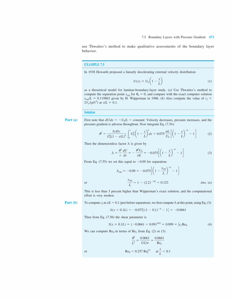
EXAMPLE 7.5

In 1938 Howarth proposed a linearly decelerating external velocity distribution

U(x) 5 U0 a1 2x

Lb (1)

as a theoretical model for laminar-boundary-layer study. (a) Use Thwaites’s method to compute the separation point xsep for θ0 5 0, and compare with the exact computer solution xsep/L 5 0.119863 given by H. Wipperman in 1966. (b) Also compute the value of cf 5 2τw/(ρU2) at x/L 5 0.1.

Solution

Part (a) First note that dU/dx 5 2U0/L 5 constant: Velocity decreases, pressure increases, and the pressure gradient is adverse throughout. Now integrate Eq. (7.54):

θ2 50.45v

U06(1 2 x/L)6 #

x

0

U05 a1 2

x

Lb5

dx 5 0.075 νL

U0 c a1 2

x

Lb26

2 1 d (2)

Then the dimensionless factor λ is given by

λ 5θ2

v dU

dx5 2

θ2U0

νL5 20.075 c a1 2

x

Lb26

2 1 d (3)

From Eq. (7.55) we set this equal to 20.09 for separation:

λsep 5 20.09 5 20.075 c a1 2xsep

Lb26

2 1 dor

xsep

L5 1 2 (2.2)21/6 5 0.123 Ans. (a)

This is less than 3 percent higher than Wipperman’s exact solution, and the computational effort is very modest.

Part (b) To compute cf at x/L 5 0.1 (just before separation), we fi rst compute λ at this point, using Eq. (3):

λ(x 5 0.1L) 5 20.075 3 (1 2 0.1)26 2 1 4 5 20.0661

Then from Eq. (7.56) the shear parameter is

S(x 5 0.1L) 5 (20.0661 1 0.09)0.62 5 0.099 5 12cf Reθ (4)

We can compute Reθ in terms of ReL from Eq. (2) or (3):

θ2

L2 50.0661

UL/ν5

0.0661

ReL

or Reθ 5 0.257 ReL1/2 at

x

L5 0.1


Substitute into Eq. (4):

0.099 5 12 cf

(0.257 ReL1/2)

or cf 50.77

ReL1/2 ReL 5

UL

ν Ans. (b)

We cannot actually compute cf without the value of, say, U0L/ν.

7.6 Experimental External Flows

Boundary layer theory is very interesting and illuminating and gives us a great qualita-tive grasp of viscous fl ow behavior; but, because of fl ow separation, the theory does not generally allow a quantitative computation of the complete fl ow fi eld. In particu-lar, there is at present no satisfactory theory, except CFD results, for the forces on an arbitrary body immersed in a stream fl owing at an arbitrary Reynolds number. There-fore, experimentation is the key to treating external fl ows. Literally thousands of papers in the literature report experimental data on specifi c external viscous fl ows. This section gives a brief description of the following external fl ow problems:

1. Drag of two- and three-dimensional bodies:

a. Blunt bodies.

b. Streamlined shapes.

2. Performance of lifting bodies:

a. Airfoils and aircraft.

b. Projectiles and fi nned bodies.

c. Birds and insects.

For further reading see the goldmine of data compiled in Hoerner [12]. In later chapters we shall study data on supersonic airfoils (Chap. 9), open-channel friction (Chap. 10), and turbomachinery performance (Chap. 11).

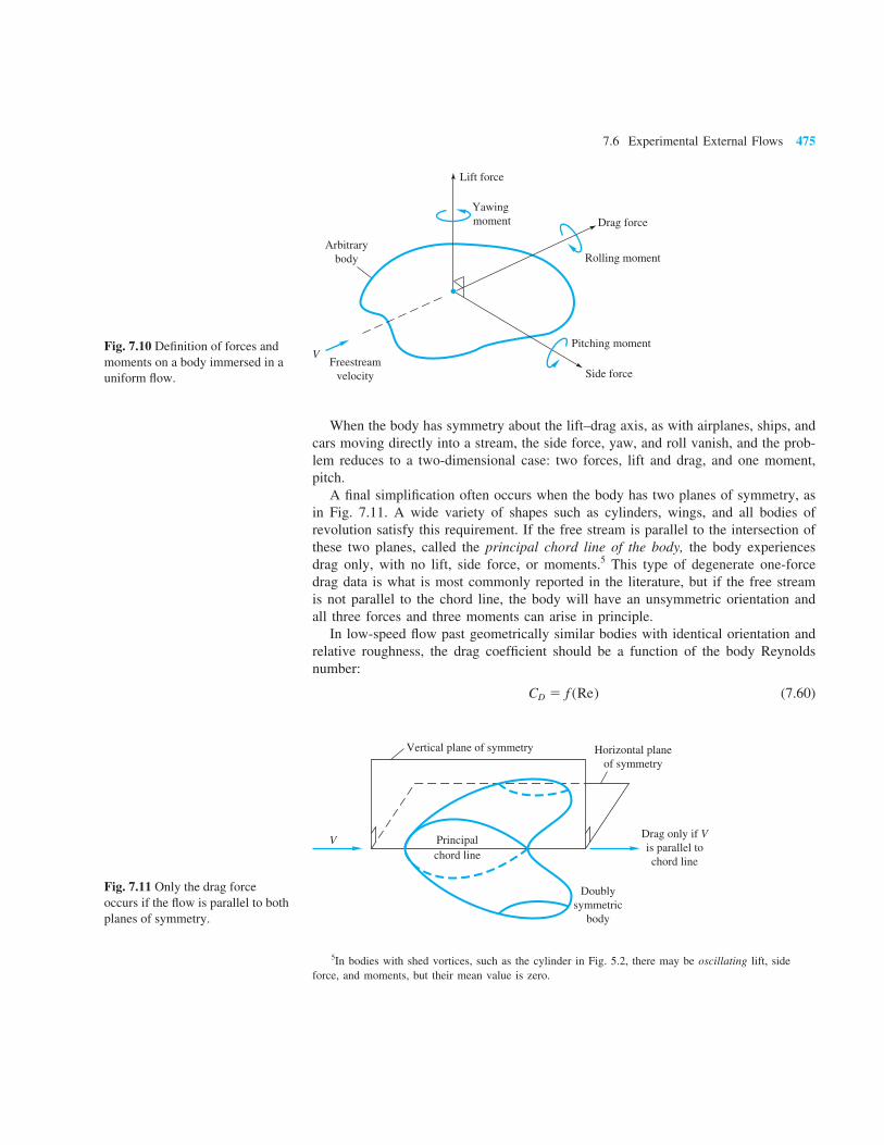
Drag of Immersed Bodies Any body of any shape when immersed in a fl uid stream will experience forces and moments from the fl ow. If the body has arbitrary shape and orientation, the fl ow will exert forces and moments about all three coordinate axes, as shown in Fig. 7.10. It is customary to choose one axis parallel to the free stream and positive downstream. The force on the body along this axis is called drag, and the moment about that axis the rolling moment. The drag is essentially a fl ow loss and must be overcome if the body is to move against the stream. A second and very important force is perpendicular to the drag and usually per-forms a useful job, such as bearing the weight of the body. It is called the lift. The moment about the lift axis is called yaw. The third component, neither a loss nor a gain, is the side force, and about this axis is the pitching moment. To deal with this three-dimensional force-moment situ-ation is more properly the role of a textbook on aerodynamics [for example, 13]. We shall limit the discussion here to lift and drag.

7.6 Experimental External Flows 475

When the body has symmetry about the lift–drag axis, as with airplanes, ships, and cars moving directly into a stream, the side force, yaw, and roll vanish, and the prob-lem reduces to a two-dimensional case: two forces, lift and drag, and one moment, pitch. A fi nal simplifi cation often occurs when the body has two planes of symmetry, as in Fig. 7.11. A wide variety of shapes such as cylinders, wings, and all bodies of revolution satisfy this requirement. If the free stream is parallel to the intersection of these two planes, called the principal chord line of the body, the body experiences drag only, with no lift, side force, or moments.5 This type of degenerate one-force drag data is what is most commonly reported in the literature, but if the free stream is not parallel to the chord line, the body will have an unsymmetric orientation and all three forces and three moments can arise in principle. In low-speed fl ow past geometrically similar bodies with identical orientation and relative roughness, the drag coeffi cient should be a function of the body Reynolds number:

CD 5 f (Re) (7.60)

Arbitrarybody

Lift force

Yawing moment Drag force

Rolling moment

Pitching moment

Side forceFreestream

velocity

VFig. 7.10 Defi nition of forces and moments on a body immersed in a uniform fl ow.

5In bodies with shed vortices, such as the cylinder in Fig. 5.2, there may be oscillating lift, side force, and moments, but their mean value is zero.

Fig. 7.11 Only the drag force occurs if the fl ow is parallel to both planes of symmetry.

V

Vertical plane of symmetry Horizontal planeof symmetry

Principalchord line

Doublysymmetric

body

Drag only if Vis parallel tochord line


The Reynolds number is based upon the free-stream velocity V and a characteristic length L of the body, usually the chord or body length parallel to the stream:

Re 5VL

ν (7.61)

For cylinders, spheres, and disks, the characteristic length is the diameter D.

Characteristic Area Drag coeffi cients are defi ned by using a characteristic area A, which may differ depending on the body shape:

CD 5drag

12 ρV2A

(7.62)

The factor 12 is our traditional tribute to Euler and Bernoulli. The area A is usually

one of three types:

1. Frontal area, the body as seen from the stream; suitable for thick, stubby bodies, such as spheres, cylinders, cars, trucks, missiles, projectiles, and torpedoes.

2. Planform area, the body area as seen from above; suitable for wide, fl at bodies such as wings and hydrofoils.

3. Wetted area, customary for surface ships and barges.

In using drag or other fl uid force data, it is important to note what length and area are being used to scale the measured coeffi cients.

Friction Drag and Pressure Drag As we have mentioned, the theory of drag is weak and inadequate, except for the fl at plate. This is because of fl ow separation. Boundary layer theory can predict the sepa-ration point but cannot accurately estimate the (usually low) pressure distribution in the separated region. The difference between the high pressure in the front stagnation region and the low pressure in the rear separated region causes a large drag contribu-tion called pressure drag. This is added to the integrated shear stress or friction dragof the body, which it often exceeds:

CD 5 CD,press 1 CD,fric (7.63)

The relative contribution of friction and pressure drag depends upon the body’s shape, especially its thickness. Figure 7.12 shows drag data for a streamlined cyl-inder of very large depth into the paper. At zero thickness the body is a fl at plate and exhibits 100 percent friction drag. At thickness equal to the chord length, simu-lating a circular cylinder, the friction drag is only about 3 percent. Friction and pressure drag are about equal at thickness t/c 5 0.25. Note that CD in Fig. 7.12blooks quite different when based on frontal area instead of planform area, planform being the usual choice for this body shape. The two curves in Fig. 7.12b represent exactly the same drag data.


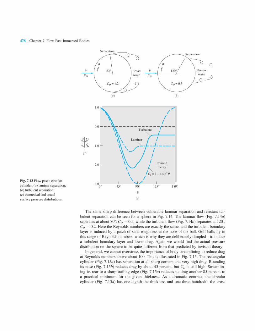
Figure 7.13 illustrates the dramatic effect of separated fl ow and the subsequent failure of boundary layer theory. The theoretical inviscid pressure distribution on a circular cylinder (Chap. 8) is shown as the dashed line in Fig. 7.13c:

Cp 5p 2 pq

12 ρV2 5 1 2 4 sin2 θ

where Pq and V are the pressure and velocity, respectively, in the free stream. The actual laminar and turbulent boundary layer pressure distributions in Fig. 7.13c are startlingly different from those predicted by theory. Laminar fl ow is very vulnerable to the adverse gradient on the rear of the cylinder, and separation occurs at θ 5 828, which certainly could not have been predicted from inviscid theory. The broad wake and very low pressure in the separated laminar region cause the large drag CD 5 1.2. The turbulent boundary layer in Fig. 7.13b is more resistant, and separation is delayed until θ 5 1208, with a resulting smaller wake, higher pressure on the rear, and 75 percent less drag, CD 5 0.3. This explains the sharp drop in drag at transition in Fig. 5.3.

0.3

0.2

0.1

00

CD

0.2 0.4 0.6 0.8 1.0

Circular cylinder

CD based on frontal area (tb)

CD based on planform area (cb)

Width b

tV

c

Thickness ratio tc

(b)

Flatplate

100

50

00 0.2 0.4 0.6 0.8 1.0(a)

3

Percentage ofpressure

drag

Data scatter

Fric

tion

drag

per

cent

tc

Fig. 7.12 Drag of a streamlined two-dimensional cylinder at Rec 5 106: (a) effect of thickness ratio on percentage of friction drag; (b) total drag versus thickness when based on two different areas.


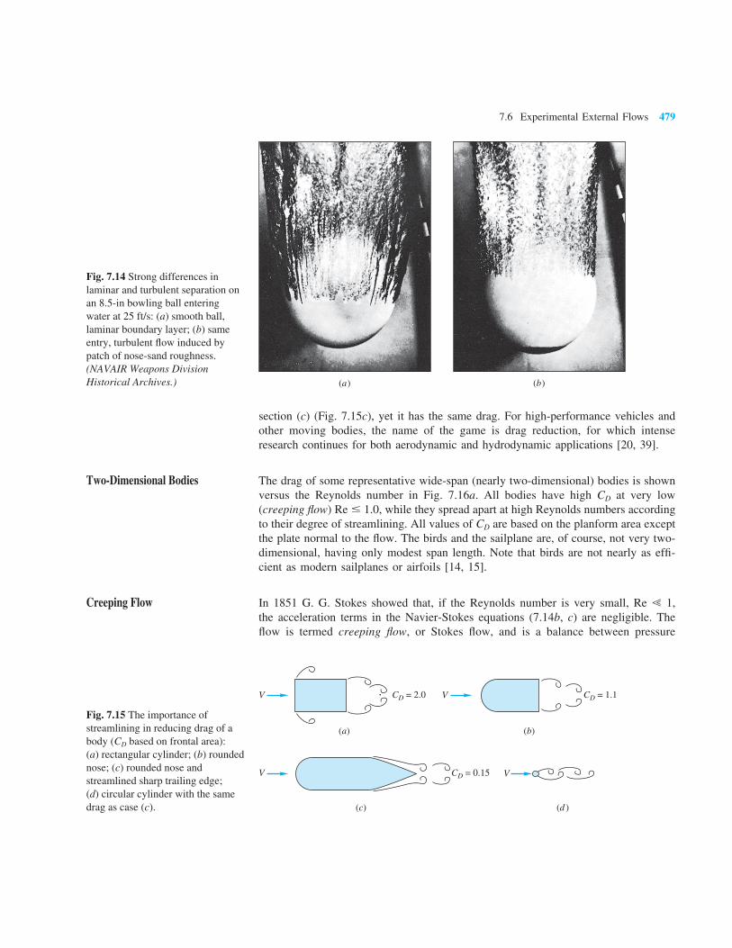
The same sharp difference between vulnerable laminar separation and resistant tur-bulent separation can be seen for a sphere in Fig. 7.14. The laminar fl ow (Fig. 7.14a) separates at about 808, CD 5 0.5, while the turbulent fl ow (Fig. 7.14b) separates at 1208, CD 5 0.2. Here the Reynolds numbers are exactly the same, and the turbulent boundary layer is induced by a patch of sand roughness at the nose of the ball. Golf balls fl y in this range of Reynolds numbers, which is why they are deliberately dimpled—to induce a turbulent boundary layer and lower drag. Again we would fi nd the actual pressure distribution on the sphere to be quite different from that predicted by inviscid theory. In general, we cannot overstress the importance of body streamlining to reduce drag at Reynolds numbers above about 100. This is illustrated in Fig. 7.15. The rectangular cylinder (Fig. 7.15a) has separation at all sharp corners and very high drag. Rounding its nose (Fig. 7.15b) reduces drag by about 45 percent, but CD is still high. Streamlin-ing its rear to a sharp trailing edge (Fig. 7.15c) reduces its drag another 85 percent to a practical minimum for the given thickness. As a dramatic contrast, the circular cylinder (Fig. 7.15d) has one-eighth the thickness and one-three-hundredth the cross

Separation

Vp∞

Broadwake

θ θ

82°

CD = 1.2

(a)

Separation

Vp∞

Narrowwake

120°

CD = 0.3

(b)

1.0

0.0

–1.0

–2.0

–3.00° 45° 90° 135° 180°

(c)

Turbulent

Laminar

Inviscidtheory

Cp = 1 – 4 sin2

Cp =

p –

p ∞ρ

V

2 / 2

θ

θ

Fig. 7.13 Flow past a circular cylinder: (a) laminar separation; (b) turbulent separation; (c) theoretical and actual surface pressure distributions.


section (c) (Fig. 7.15c), yet it has the same drag. For high-performance vehicles and other moving bodies, the name of the game is drag reduction, for which intense research continues for both aerodynamic and hydrodynamic applications [20, 39].

Two-Dimensional Bodies The drag of some representative wide-span (nearly two-dimensional) bodies is shown versus the Reynolds number in Fig. 7.16a. All bodies have high CD at very low (creeping fl ow) Re # 1.0, while they spread apart at high Reynolds numbers according to their degree of streamlining. All values of CD are based on the planform area except the plate normal to the fl ow. The birds and the sailplane are, of course, not very two-dimensional, having only modest span length. Note that birds are not nearly as effi -cient as modern sailplanes or airfoils [14, 15].

Creeping Flow In 1851 G. G. Stokes showed that, if the Reynolds number is very small, Re ! 1, the acceleration terms in the Navier-Stokes equations (7.14b, c) are negligible. The fl ow is termed creeping fl ow, or Stokes fl ow, and is a balance between pressure

(b )(a )

Fig. 7.14 Strong differences in laminar and turbulent separation on an 8.5-in bowling ball entering water at 25 ft/s: (a) smooth ball, laminar boundary layer; (b) same entry, turbulent fl ow induced by patch of nose-sand roughness. (NAVAIR Weapons Division Historical Archives.)

V

(a)

CD = 1.1

V

(c)

CD = 2.0 V

(b)

CD = 0.15 V

(d )

Fig. 7.15 The importance of streamlining in reducing drag of a body (CD based on frontal area): (a) rectangular cylinder; (b) rounded nose; (c) rounded nose and streamlined sharp trailing edge; (d) circular cylinder with the same drag as case (c).


gradient and viscous stresses. Continuity and momentum reduce to two linear equa-tions for velocity and pressure:

Re ! 1: = ? V 5 0 and §p < μ§ 2V

If the geometry is simple (for example, a sphere or disk), closed-form solutions can be found and the body drag can be computed [2]. Stokes himself provided the sphere drag formula:

Fsphere 5 3π μUd

or CD 5F

12 ρU2 π4 d2 5

24

ρUd/μ5

24

Red (7.64)

This relation is plotted in Fig. 7.16b and is seen to be accurate for about Red # 1.

10

100

10

1

0.1

0.01

0.0010.1 1 10 100 103 104 105 106 107

Re

Airfoil

Seagull

Sailplane

CD

Stokes’slaw:

24/Re

Disk normal tostream

(a)

100

10

1

0.1

0.01

CD

0.1 1 100 103 104 105 106 107

Re

(b)

Smoothflat plateparallel

to stream

LD

= ∞

= 5

Smoothcircularcylinder

Squarecylinder

Platenormal

to stream

Transition

Pigeon

Vulture

2:1Ellipsoid

Airship hull

Sphere

Fig. 7.16 Drag coeffi cients of smooth bodies at low Mach numbers: (a) two-dimensional bodies; (b) three-dimensional bodies. Note the Reynolds number independence of blunt bodies at high Re.


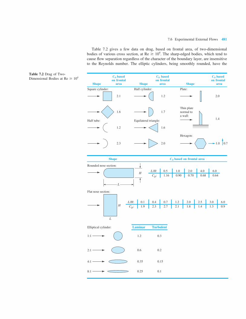
Table 7.2 gives a few data on drag, based on frontal area, of two-dimensional bodies of various cross section, at Re $ 104. The sharp-edged bodies, which tend to cause fl ow separation regardless of the character of the boundary layer, are insensitive to the Reynolds number. The elliptic cylinders, being smoothly rounded, have the

C D based C D based C D based on frontal on frontal on frontal Shape area Shape area Shape area

Shape C D based on frontal area

Table 7.2 Drag of Two-Dimensional Bodies at Re $ 104

Square cylinder:

Half tube:

Half cylinder:

Equilateral triangle:

2.1

1.6

1.2

2.3

1.2

1.7

1.6

2.0

2.0

1.4

1.0 0.7

Plate:

Thin plate normal to a wall:

Hexagon:

L

H

Rounded nose section:

0.51.16

1.00.90

2.00.70

4.00.68

6.00.64

H

L

Flat nose section:

L /H:

0.11.9

0.42.3

0.72.7

1.22.1

2.01.8

2.51.4

3.01.3

6.00.9

Elliptical cylinder: Laminar

1.2

0.6

0.35

0.25

Turbulent

0.3

0.2

0.15

0.1

1:1

2:1

4:1

8:1

CD:

L /H: CD:


laminar-to-turbulent transition effect of Figs. 7.13 and 7.14 and are therefore quite sensitive to whether the boundary layer is laminar or turbulent.

EXAMPLE 7.6

A square 6-in piling is acted on by a water fl ow of 5 ft/s that is 20 ft deep, as shown in Fig. E7.6. Estimate the maximum bending exerted by the fl ow on the bottom of the piling.

Solution

Assume seawater with ρ 5 1.99 slugs/ft3 and kinematic viscosity ν 5 0.000011 ft2/s. With a piling width of 0.5 ft, we have

Reh 5(5 ft/s) (0.5 ft)

0.000011 ft2/s5 2.3 3 105

This is the range where Table 7.2 applies. The worst case occurs when the fl ow strikes the fl at side of the piling, CD < 2.1. The frontal area is A 5 Lh 5 (20 ft)(0.5 ft) 5 10 ft2. The drag is estimated by

F 5 CD (12 ρV2A) < 2.1(1

2) (1.99 slugs/ft3) (5 ft/s)2 (10 ft2) 5 522 lbf

If the fl ow is uniform, the center of this force should be at approximately middepth. There-fore, the bottom bending moment is

M0 <FL

25 522(10) 5 5220 ft ? lbf Ans.

According to the fl exure formula from strength of materials, the bending stress at the bottom would be

S 5M0y

I5

(5220 ft # lb)(0.25 ft)1

12(0.5 ft)4 5 251,000 lbf/ft2 5 1740 lbf/in2

to be multiplied, of course, by the stress concentration factor due to the built-in end conditions.

Three-Dimensional Bodies Some drag coeffi cients of three-dimensional bodies are listed in Table 7.3 and Fig. 7.16b. Again we can conclude that sharp edges always cause fl ow separation and high drag

L = 20 ft5 ft/s

h = 6 in

E7.6


Cube:

1.07 [60]

0.81

Cup:

1.4

0.4

1.17

Disk:

1.2

Parachute (Low porosity):

Rectangular plate:

h

h

b ∞

b/h 15

1020

1.181.21.31.52.0

L/D:CD:

10.64

20.68

30.72

50.74

100.82

200.91

400.98

∞1.20

L

D

Short cylinder, laminar flow:

Porous parabolic dish [23]: Porosity: 0

1.420.95

0.11.330.92

0.21.200.90

0.31.050.86

0.40.950.83

0.50.820.80

Flat-faced cylinder:

Ellipsoid:

L /d 0.51248

1.150.900.850.870.99

L /d 0.75

Laminar

0.50.470.270.250.2

Turbulent

0.20.20.130.10.08

1248

d

L

CD

A = 9 ft2

CD

A = 8.5 m2

Upright: CD

A = 0.51 m2; Racing: CD

A = 0.30 m2

C D

A = 1.2 ft2

Average person:

U, m/s:CD:

101.2 ± 0.2

201.0 ± 0.2

300.7 ± 0.2

400.5 ± 0.2

Pine and spruce trees [24]:

Buoyant rising sphere [50],

135 < Red < 1E5

CD ≈ 0.95

Cone:10°0.30

20°0.40

30°0.55

40°0.65

60°0.80

75°1.05

90°1.15

θθ :CD:

CD:

CD:

Tractor-trailer truck: Without deflector: 0.96; with deflector: 0.76

Streamlined train (approximately 5 cars):

Bicycle:

C D based on Body frontal area Body C D based on frontal area

Table 7.3 Drag of Three-Dimensional Bodies at Re $ 104

C D based on C D based on Body Ratio frontal area Body Ratio frontal area


that is insensitive to the Reynolds number. Rounded bodies like the ellipsoid have drag that depends on the point of separation, so both the Reynolds number and the character of the boundary layer are important. Body length will generally decrease pressure drag by making the body relatively more slender, but sooner or later the friction drag will catch up. For the fl at-faced cylinder in Table 7.3, pressure drag decreases with L/d but friction increases, so minimum drag occurs at about L/d 5 2.

Buoyant Rising Light Spheres The sphere data in Fig. 7.16b are for fi xed models in wind tunnels and from falling sphere tests and indicate a drag coeffi cient of about 0.5 in the range 1 E3 , Red , 1 E5. It was pointed out [50] that this is not the case for a freely rising buoyant sphere or bubble. If the sphere is light, ρsphere , 0.8 ρfl uid, a wake instability arises in the range 135 , Red , 1 E5. The sphere then spirals upward at an angle of about 608 from the horizontal. The drag coeffi cient is approximately doubled, to an average value CD < 0.95, as listed in Table 7.3 [50]. For a heavier body, ρsphere < ρfl uid, the buoyant sphere rises vertically and the drag coeffi cient follows the standard curve in Fig. 7.16b.

EXAMPLE 7.7

According to Ref. 12, the drag coeffi cient of a blimp, based on surface area, is approximately 0.006 if ReL . 106. A certain blimp is 75 m long and has a surface area of 3400 m2. Esti-mate the power required to propel this blimp at 18 m/s at a standard altitude of 1000 m.

Solution

• Assumptions: We hope the Reynolds number will be high enough that the given data are valid.

• Approach: Determine if ReL . 106 and, if so, compute the drag and the power required.• Property values: Table A.6 at z 5 1000 m: ρ 5 1.112 kg/m3, T 5 282 K, thus μ <

1.75 E-5 kg/m ? s.• Solution steps: Determine the Reynolds number of the blimp:

ReL 5ρUL

μ5

(1.112 kg/m3)(18 m/s)(75 m)

1.75 E-5 kg/m # s5 8.6 E7 . 106 OK

The given drag coeffi cient is valid. Compute the blimp drag and the power 5 (drag) 3 (velocity):

F 5 CD ρ

2 U2Awet 5 (0.006)

1.112 kg/m3

2 (18 m/s)2 (3400 m2) 5 3675 N

Power 5 FV 5 (3675 N)(18 m/s) 5 66,000 W (89 hp) Ans.

• Comments: These are nominal estimates. Drag is highly dependent on both shape and Reynolds number, and the coeffi cient CD 5 0.006 has considerable uncertainty.

Aerodynamic Forces on Road Vehicles

Automobiles and trucks are now the subject of much research on aerodynamic forces, both lift and drag [21]. At least one textbook is devoted to the subject [22]. A very readable description of race car drag is given by Katz [51]. Consumer, manufacturer, and government interest has cycled between high speed/high horsepower and lower


speed/lower drag. Better streamlining of car shapes has resulted over the years in a large decrease in the automobile drag coeffi cient, as shown in Fig. 7.17a. Modern cars have an average drag coeffi cient of about 0.25, based on the frontal area. Since the frontal area has also decreased sharply, the actual raw drag force on cars has dropped even more than indicated in Fig. 7.17a. The theoretical minimum shown in the fi gure, CD < 0.15, is about right for a commercial automobile, but lower values are possible for experimental vehicles; see Prob. P7.109. Note that basing CD on the frontal area is awkward, since one would need an accurate drawing of the automobile to estimate its frontal area. For this reason, some technical articles simply report the raw drag in newtons or pound-force, or the product CDA. Many companies and laboratories have automotive wind tunnels, some full-scale and/or with moving fl oors to approximate actual kinematic similarity. The blunt shapes of most automobiles, together with their proximity to the ground, cause a wide variety of fl ow and geometric effects. Simple changes in part of the shape can have

1900 1910 1920 1930 1940 1950 1960 1970 1980 1990 2000

Year

(a)

1.2

1.0

0.8

0.6

0.4

0.2

0.0

(b)

Upsweep angle , deg

1.0

0.9

0.8

0.7

0.6

0.5

0.4

0.3

0.2

0.1

0

CD

0.15

0 5 10 15 20 25 30 35 40

Downward forcecoefficient

Drag coefficient

Theoreticalminimum

θ

θ

Fig. 7.17 Aerodynamics of automobiles: (a) the historical trend for drag coeffi cients (from Ref. 21); (b) effect of bottom rear upsweep angle on drag and downward lift force (from Ref. 25).


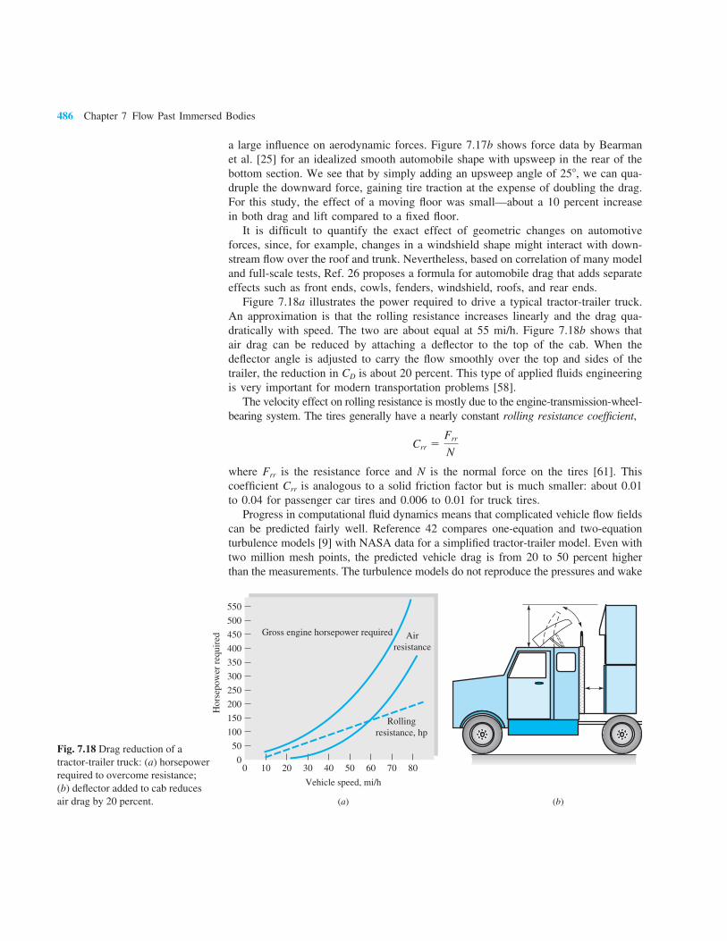
a large infl uence on aerodynamic forces. Figure 7.17b shows force data by Bearman et al. [25] for an idealized smooth automobile shape with upsweep in the rear of the bottom section. We see that by simply adding an upsweep angle of 258, we can qua-druple the downward force, gaining tire traction at the expense of doubling the drag. For this study, the effect of a moving fl oor was small—about a 10 percent increase in both drag and lift compared to a fi xed fl oor. It is diffi cult to quantify the exact effect of geometric changes on automotive forces, since, for example, changes in a windshield shape might interact with down-stream fl ow over the roof and trunk. Nevertheless, based on correlation of many model and full-scale tests, Ref. 26 proposes a formula for automobile drag that adds separate effects such as front ends, cowls, fenders, windshield, roofs, and rear ends. Figure 7.18a illustrates the power required to drive a typical tractor-trailer truck. An approximation is that the rolling resistance increases linearly and the drag qua-dratically with speed. The two are about equal at 55 mi/h. Figure 7.18b shows that air drag can be reduced by attaching a defl ector to the top of the cab. When the defl ector angle is adjusted to carry the fl ow smoothly over the top and sides of the trailer, the reduction in CD is about 20 percent. This type of applied fl uids engineering is very important for modern transportation problems [58]. The velocity effect on rolling resistance is mostly due to the engine-transmission-wheel-bearing system. The tires generally have a nearly constant rolling resistance coeffi cient,

Crr 5Frr

N

where Frr is the resistance force and N is the normal force on the tires [61]. This coeffi cient Crr is analogous to a solid friction factor but is much smaller: about 0.01 to 0.04 for passenger car tires and 0.006 to 0.01 for truck tires. Progress in computational fl uid dynamics means that complicated vehicle fl ow fi elds can be predicted fairly well. Reference 42 compares one-equation and two-equation turbulence models [9] with NASA data for a simplifi ed tractor-trailer model. Even with two million mesh points, the predicted vehicle drag is from 20 to 50 percent higher than the measurements. The turbulence models do not reproduce the pressures and wake

Hor

sepo

wer

req

uire

d

0 20 30 40 50 60 70 8010

Vehicle speed, mi/h

(a) (b)

Gross engine horsepower required Airresistance

Rollingresistance, hp

550

500

450

400

350

300

250

200

150

100

50

0Fig. 7.18 Drag reduction of a tractor-trailer truck: (a) horsepower required to overcome resistance; (b) defl ector added to cab reduces air drag by 20 percent.


structure in the rear of the vehicle. Newer models, such as large eddy simulation (LES) and direct numerical simulation (DNS) will no doubt improve the calculations.

EXAMPLE 7.8

A high-speed car with m 5 2000 kg, CD 5 0.3, and A 5 1 m2 deploys a 2-m parachute to slow down from an initial velocity of 100 m/s (Fig. E7.8). Assuming constant CD, brakes free, and no rolling resistance, calculate the distance and velocity of the car after 1, 10, 100, and 1000 s. For air assume ρ 5 1.2 kg/m3, and neglect interference between the wake of the car and the parachute.

Solution

Newton’s law applied in the direction of motion gives

Fx 5 m dV

dt5 2Fc 2 Fp 5 2

1

2 ρV2(CDc Ac 1 CDp Ap)

where subscript c denotes the car and subscript p the parachute. This is of the form

dV

dt5 2

K

m V2 K 5 a CDA

ρ

2

Separate the variables and integrate:

#v

v0

dV

V2 5 2K

m #

t

0

dt

or V 021 2 V 21 5 2

K

m t

Rearrange and solve for the velocity V:

V 5V0

1 1 (K/m)V0t K 5

(CDc Ac 1 CDp Ap)ρ

2 (1)

We can integrate this to fi nd the distance traveled:

S 5V0

α 1n (1 1 αt) α 5

K

m V0 (2)

Now work out some numbers. From Table 7.3, CDp < 1.2; hence

CDc Ac 1 CDp Ap 5 0.3(1 m2) 1 1.2 π

4 (2 m)2 5 4.07 m2

Then K

m V0 5

12 (4.07 m2)(1.2 kg/m3)(100 m/s)

2000 kg5 0.122 s21 5 α

Now make a table of the results for V and S from Eqs. (1) and (2):

d p = 2 m V0 = 100 m/s

xE7.8


t, s 1 10 100 1000

V , m/s 89 45 7.6 0.8

S , m 94 654 2110 3940

Air resistance alone will not stop a body completely. If you don’t apply the brakes, you’ll be halfway to the Yukon Territory and still going.

Other Methods of Drag Reduction Sometimes drag is good, for example, when using a parachute. Do not jump out of an airplane holding a fl at plate parallel to your motion (see Prob. P7.81). Mostly, though, drag is bad and should be reduced. The classical method of drag reduction is streamlining (Figs. 7.15 and 7.18). For example, nose fairings and body panels have produced motorcycles that can travel over 200 mi/h. More recent research has uncovered other methods that hold great promise, especially for turbulent fl ows.

1. Oil pipelines introduce an annular strip of water to reduce the pumping power [36]. The low-viscosity water rides the wall and reduces friction up to 60 percent.

2. Turbulent friction in liquid flows is reduced up to 60 percent by dissolving small amounts of a high-molecular-weight polymer additive [37]. Without changing pumps, the Trans-Alaska Pipeline System (TAPS) increased oil flow 50 percent by injecting small amounts of polymer dissolved in kerosene.

3. Stream-oriented surface vee-groove microriblets can reduce turbulent friction up to 8 percent [38]. Riblet heights are of order 1 mm and were used on the Stars and Stripes yacht hull in the Americas Cup races. Riblets are also effective on aircraft skins.

4. Small, near-wall large-eddy breakup devices (LEBUs) reduce local turbulent friction up to 10 percent [39]. However, one must add these small structures to the surface, and LEBU drag may be signifi cant.

5. Air microbubbles injected at the wall of a water fl ow create a low-shear bubble blanket [40]. At high void fractions, drag reduction can be 80 percent.

6. Spanwise (transverse) wall oscillation may reduce turbulent friction up to 30 percent [41].

7. Active fl ow control, especially of turbulent fl ows, is the wave of the future, as reviewed in Ref. 47. These methods generally require expenditure of energy but can be worth it. For example, tangential blowing at the rear of an auto [48] evokes the Coanda effect, in which the separated near-wake fl ow attaches itself to the body surface and reduces auto drag up to 10 percent.

Drag reduction is presently an area of intense and fruitful research and applies to many types of airfl ows [39, 53] and water fl ows for both vehicles and conduits.

Drag of Surface Ships The drag data given so far, such as Tables 7.2 and 7.3, are for bodies “fully immersed” in a free stream—that is, with no free surface. If, however, the body moves at or near


a free liquid surface, wave-making drag becomes important and is dependent on both the Reynolds number and the Froude number. To move through a water surface, a ship must create waves on both sides. This implies putting energy into the water surface and requires a fi nite drag force to keep the ship moving, even in a frictionless fl uid. The total drag of a ship can then be approximated as the sum of friction drag and wave-making drag:

F < Ffric 1 Fwave or CD < CD,fric 1 CD,wave

The friction drag can be estimated by the (turbulent) fl at-plate formula, Eq. (7.45), based on the below-water or wetted area of the ship. Reference 27 is an interesting review of both theory and experiment for wake-making surface ship drag. Generally speaking, the bow of the ship creates a wave system whose wavelength is related to the ship speed but not necessarily to the ship length. If the stern of the ship is a wave trough, the ship is essentially climbing uphill and has high wave drag. If the stern is a wave crest, the ship is nearly level and has lower drag. The criterion for these two conditions results in certain approximate Froude numbers [27]:

Fr 5V

1gL<

0.53

1N high drag if N 5 1, 3, 5, 7, p ;

low drag if N 5 2, 4, 6, 8, p (7.65)

where V is the ship’s speed, L is the ship’s length along the centerline, and N is the number of half-lengths, from bow to stern, of the drag-making wave system. The wave drag will increase with the Froude number and oscillate between lower drag (Fr < 0.38, 0.27, 0.22, . . .) and higher drag (Fr < 0.53, 0.31, 0.24, . . .) with neg-ligible variation for Fr , 0.2. Thus it is best to design a ship to cruise at N 5 2, 4, 6, 8. Shaping the bow and stern can further reduce wave-making drag. Figure 7.19 shows the data of Inui [27] for a model ship. The main hull, curve A, shows peaks and valleys in wave drag at the appropriate Froude numbers . 0.2. Introduction of a bulb protrusion on the bow, curve B, greatly reduces the drag. Add-ing a second bulb to the stern, curve C, is still better, and Inui recommends that the design speed of this two-bulb ship be at N 5 4, Fr < 0.27, which is a nearly “wave-less” condition. In this fi gure CD,wave is defi ned as 2Fwave/(ρV2L2) instead of using the wetted area. The solid curves in Fig. 7.19 are based on potential fl ow theory for the below-water hull shape. Chapter 8 is an introduction to potential fl ow theory. Modern computers can be programmed for numerical CFD solutions of potential fl ow over the hulls of ships, submarines, yachts, and sailboats, including boundary layer effects driven by the potential fl ow [28]. Thus theoretical prediction of fl ow past surface ships is now at a fairly high level. See also Ref. 15.

Body Drag at High Mach Numbers

All the data presented to this point are for nearly incompressible fl ows, with Mach numbers assumed less than about 0.3. Beyond this value compressibility can be very important, with CD 5 fcn(Re, Ma). As the stream Mach number increases, at some subsonic value Mcrit , 1 that depends on the body’s bluntness and thickness, the local velocity at some point near the body surface will become sonic. If Ma increases beyond Macrit, shock waves form, intensify, and spread, raising surface


pressures near the front of the body and therefore increasing the pressure drag. The effect can be dramatic with CD increasing tenfold, and 70 years ago this sharp increase was called the sonic barrier, implying that it could not be surmounted. Of course, it can be—the rise in CD is fi nite, as supersonic bullets have proved for centuries. Figure 7.20 shows the effect of the Mach number on the drag coeffi cient of various body shapes tested in air.6 We see that compressibility affects blunt bodies earlier, with Macrit equal to 0.4 for cylinders, 0.6 for spheres, and 0.7 for airfoils and pointed projectiles. Also the Reynolds number (laminar versus turbulent boundary layer fl ow) has a large effect below Macrit for spheres and cylinders but becomes unimportant above Ma < 1. In contrast, the effect of the Reynolds number is small for airfoils and projectiles and is not shown in Fig. 7.20. A general statement might divide Reynolds and Mach number effects as follows:

Ma # 0.3: Reynolds number important, Mach number unimportant

0.3 , Ma , 1: both Reynolds and Mach numbers important

Ma . 1.0: Reynolds number unimportant, Mach number important

At supersonic speeds, a broad bow shock wave forms in front of the body (see Figs. 9.10b and 9.19), and the drag is mainly due to high shock-induced pressures on the front. Making the bow a sharp point can sharply reduce the drag (Fig. 9.28) but

0.10 0.20 0.30 0.40 0.50

Designspeed

Potential flow theory

A Main hull (without bulb)B With bow bulb

C With bow and stern-bulbs

A

B

C

Fr = V

√Lg

0.002

0.001

0

CD,wave

0.60Fig. 7.19 Wave-making drag on a ship model. (After Inui [27].) Note: The drag coeffi cient is defi ned as CDW 5 2F/(ρV2L2).

6There is a slight effect of the specifi c-heat ratio k, which would appear if other gases were tested.


does not eliminate the bow shock. Chapter 9 gives a brief treatment of compressible fl ow. References 30 and 31 are more advanced textbooks devoted entirely to com-pressible fl ow.

Biological Drag Reduction A great deal of engineering effort goes into designing immersed bodies to reduce their drag. Most such effort concentrates on rigid-body shapes. A different process occurs in nature, as organisms adapt to survive high winds or currents, as reported in a series of papers by S. Vogel [33, 34]. A good example is a tree, whose fl exible structure allows it to reconfi gure in high winds and thus reduce drag and damage. Tree root systems have evolved in several ways to resist wind-induced bending moments, and trunk cross sections have become resistant to bending but relatively easy to twist and reconfi gure. We saw this in Table 7.3, where tree drag coeffi cients [24] reduced by 60 percent as wind velocity increased. The shape of the tree changes to offer less resistance. The individual branches and leaves of a tree also curl and cluster to reduce drag. Figure 7.21 shows the results of wind tunnel experiments by Vogel [33]. A tulip tree leaf, Fig. 7.21a, broad and open in low wind, curls into a conical low-drag shape as wind increases. A compound black walnut leaf group, Fig. 7.21b, clusters into a low-drag shape at high wind speed. Although drag coeffi cients were reduced up to 50 percent by fl exibility, Vogel points out that rigid structures are sometimes just as effective. An interesting recent symposium [35] was devoted entirely to the solid mechanics and fl uid mechanics of biological organisms.

0.0 1.0 2.0 3.0 4.0Mach number

Airfoil

Pointed bodyof revolution

SphereLaminar, Re ≈ 1 E5Turbulent, Re ≈ 1 E6

CD

Laminar, Re ≈ 1 E5

Turbulent, Re ≈ 1 E6

Cylinder in cross flow:

2.0

1.8

1.6

1.4

1.2

1.0

0.8

0.6

0.4

0.2

0.0Fig. 7.20 Effect of the Mach number on the drag of various body shapes. (Data from Refs. 23 and 29.)


Forces on Lifting Bodies Lifting bodies (airfoils, hydrofoils, or vanes) are intended to provide a large force normal to the free stream and as little drag as possible. Conventional design practice has evolved a shape not unlike a bird’s wing—that is, relatively thin (t/c # 0.24) with a rounded leading edge and a sharp trailing edge. A typical shape is sketched in Fig. 7.22. For our purposes we consider the body to be symmetric, as in Fig. 7.11, with the free-stream velocity in the vertical plane. If the chord line between the leading and trailing edge is not a line of symmetry, the airfoil is said to be cambered. The camber line is the line midway between the upper and lower surfaces of the vane. The angle between the free stream and the chord line is called the angle of attack α. The lift L and the drag D vary with this angle. The dimensionless forces are defi ned

5 m/s

10 m/s

20 m/s

(a)

5 m/s

10 m/s

20 m/s

(b)

Fig. 7.21 Biological adaptation to wind forces: (a) a tulip tree leaf curls into a conical shape at high velocity; (b) black walnut leaves cluster into a low-drag shape as wind increases. (From Vogel, Ref. 33.)

α

Planformarea = bc

Angle ofattack

V

c = chord

b = spant = thickness

Lift

Drag

Fig. 7.22 Defi nition sketch for a lifting vane.


with respect to the planform area Ap 5 bc:

Lift coeffi cient: CL 5L

12 ρV2Ap

(7.66a)

Drag coeffi cient: CD 5D

12 ρV2Ap

(7.66b)

If the chord length is not constant, as in the tapered wings of modern aircraft, Ap 5 ec db. For low-speed fl ow with a given roughness ratio, CL and CD should vary with α and the chord Reynolds number:

CL 5 f (α, Rec) or CD 5 f (α, Rec)

where Rec 5 Vc/ν. The Reynolds numbers are commonly in the turbulent boundary layer range and have a modest effect. The rounded leading edge prevents fl ow separation there, but the sharp trailing edge causes a tangential wake motion that generates the lift. Figure 7.23 shows what happens when a fl ow starts up past a lifting vane or an airfoil. Just after start-up in Fig. 7.23a the streamline motion is irrotational and inviscid. The rear stagnation point, assuming a positive angle of attack, is on the upper surface, and there is no lift; but the fl ow cannot long negotiate the sharp turn at the trailing edge: it separates, and a starting vortex forms in Fig. 7.23b. This starting vortex is shed downstream in Figs. 7.23c and d, and a smooth streamline fl ow develops over the wing, leaving the foil in a direction approximately parallel to the chord line. Lift at this time is fully developed, and the starting vortex is gone. Should the fl ow now cease, a stopping vortex of opposite (clockwise) sense will form and be shed. During fl ight, increases or decreases in lift will cause incremental starting or stopping vortices,

(a)

(b)

(c)

(d)

Fig. 7.23 Transient stages in the development of lift: (a) start-up: rear stagnation point on the upper surface: no lift; (b) sharp trailing edge induces separation, and a starting vortex forms: slight lift; (c) starting vortex is shed; and streamlines fl ow smoothly from trailing edge: lift is now 80 percent developed; (d ) starting vortex now shed far behind, trailing edge now very smooth: lift fully developed.


always with the effect of maintaining a smooth parallel fl ow at the trailing edge. We pursue this idea mathematically in Chap. 8. At a low angle of attack, the rear surfaces have an adverse pressure gradient but not enough to cause signifi cant boundary layer separation. The fl ow pattern is smooth, as in Fig. 7.23d, and drag is small and lift excellent. As the angle of attack is increased, the upper-surface adverse gradient becomes stronger, and generally a separation bub-ble begins to creep forward on the upper surface.7 At a certain angle α 5 15 to 208, the fl ow is separated completely from the upper surface, as in Fig. 7.24. The airfoil is said to be stalled: Lift drops off markedly, drag increases markedly, and the foil is no longer fl yable. Early airfoils were thin, modeled after birds’ wings. The German engineer Otto Lilienthal (1848–1896) experimented with fl at and cambered plates on a rotating arm. He and his brother Gustav fl ew the world’s fi rst glider in 1891. Horatio Frederick Phillips (1845–1912) built the fi rst wind tunnel in 1884 and measured the lift and drag of cambered vanes. The fi rst theory of lift was proposed by Frederick W. Lanchester shortly afterward. Modern airfoil theory dates from 1905, when the Russian hydro-dynamicist N. E. Joukowsky (1847–1921) developed a circulation theorem (Chap. 8) for computing airfoil lift for arbitrary camber and thickness. With this basic theory, as extended and developed by Prandtl and Kármán and their students, it is now pos-sible to design a low-speed airfoil to satisfy particular surface pressure distributions and

7For some airfoils the bubble leaps, not creeps, forward, and stall occurs rapidly and dangerously.

Fig. 7.24 At high angle of attack, smoke fl ow visualization shows stalled fl ow on the upper surface of a lifting vane. (National Committee for Fluid Mechanics Films, Education Development Center, Inc., © 1972.)


boundary layer characteristics. There are whole families of airfoil designs, notably those developed in the United States under the sponsorship of the NACA (now NASA). Extensive theory and data on these airfoils are contained in Ref. 16. We shall discuss this further in Chap. 8. The history of aeronautics is a rich and engaging topic and highly recommended to the reader [43, 44]. Figure 7.25 shows the lift and drag on a symmetric airfoil denoted as the NACA 0009 foil, the last digit indicating the thickness of 9 percent. With no fl ap extended, this airfoil, as expected, has zero lift at zero angle of attack. Up to about 128 the lift coeffi cient increases linearly with a slope of 0.1 per degree, or 6.0 per radian. This is in agreement with the theory outlined in Chap. 8:

CL,theory < 2π sin aα 12hcb (7.67)

where h/c is the maximum camber expressed as a fraction of the chord. The NACA 0009 has zero camber; hence CL 5 2π sin α < 0.11α, where α is in degrees. This is excellent agreement. The drag coeffi cient of the smooth-model airfoils in Fig. 7.25 is as low as 0.005, which is actually lower than both sides of a fl at plate in turbulent fl ow. This is mis-leading inasmuch as a commercial foil will have roughness effects; for example, a paint job will double the drag coeffi cient. The effect of increasing Reynolds number in Fig. 7.25 is to increase the maximum lift and stall angle (without changing the slope appreciably) and to reduce the drag coeffi cient. This is a salutary effect since the prototype will probably be at a higher Reynolds number than the model (107 or more). For takeoff and landing, the lift is greatly increased by defl ecting a split fl ap, as shown in Fig. 7.25. This makes the airfoil unsymmetric (or effectively cambered)

CL∞

α

6 × 10

6

3 × 10 6

–12 – 8 – 4

CD∞

– 8 – 4 0 4 8 12 160 4 8 12 16

, degα , degα

1.6

1.2

0.8

0.4

With flapat 60°

Rec = 6 × 10

6

No flap

No flap

0.01

0.02

0.03

0.04

Splitflap

Rec = 9 × 10

6

With flapat 60°

Rec = 3 × 10

6

6 × 10

6

9 × 10

6

Fig. 7.25 Lift and drag of a symmetric NACA 0009 airfoil of infi nite span, including effect of a split-fl ap defl ection. Note that roughness can increase CD from 100 to 300 percent.


and changes the zero-lift point to α 5 2128. The drag is also greatly increased by the fl ap, but the reduction in takeoff and landing distance is worth the extra power needed. A lifting craft cruises at low angle of attack, where the lift is much larger than the drag. Maximum lift-to-drag ratios for the common airfoils lie between 20 and 50. Some airfoils, such as the NACA 6 series, are shaped to provide favorable gradients over much of the upper surface at low angles. Thus separation is small, and transition to turbulence is delayed; the airfoil retains a good length of laminar fl ow even at high Reynolds numbers. The lift-drag polar plot in Fig. 7.26 shows the NACA 0009 data from Fig. 7.25 and a laminar fl ow airfoil, NACA 63-009, of the same thickness. The laminar fl ow airfoil has a low-drag bucket at small angles but also suffers lower stall angle and lower maximum lift coeffi cient. The drag is 30 percent less in the bucket, but the bucket disappears if there is signifi cant surface roughness. All the data in Figs. 7.25 and 7.26 are for infi nite span—that is, a two-dimensional fl ow pattern about wings without tips. The effect of fi nite span can be correlated with the dimensionless slenderness, or aspect ratio, denoted (AR):

AR 5b2

Ap5

b

c (7.68)

where c is the average chord length. Finite-span effects are shown in Fig. 7.27. The lift slope decreases, but the zero-lift angle is the same; and the drag increases, but the zero-lift drag is the same. The theory of fi nite-span airfoils [16] predicts that the effective angle of attack increases, as in Fig. 7.27, by the amount

¢α <CL

πAR (7.69)

1.2

0.8

0.4

00

0.008 0.016 0.024

CL

Stall

CD

Low-drag“bucket”

NACA0009

NACA63 – 009

0009 withsplit flap

Stall

Fig. 7.26 Lift-drag polar plot for standard (0009) and a laminar fl ow (63-009) NACA airfoil.


When applied to Eq. (7.67), the fi nite-span lift becomes

CL <2π sin (α 1 2h/c)

1 1 2/AR (7.70)

The associated drag increase is DCD < CL sin Dα < CL Dα, or

CD < CDq 1CL

2

πAR (7.71)

where CDq is the drag of the infi nite-span airfoil, as sketched in Fig. 7.25. These correlations are in good agreement with experiments on fi nite-span wings [16]. The existence of a maximum lift coeffi cient implies the existence of a minimum speed, or stall speed, for a craft whose lift supports its weight:

L 5 W 5 CL,max(12ρVs

2Ap)

or Vs 5 a 2W

CL,max ρApb1/2

(7.72)

The stall speed of typical aircraft varies between 60 and 200 ft/s, depending on the weight and value of CL,max. The pilot must hold the speed greater than about 1.2Vs to avoid the instability associated with complete stall. The split fl ap in Fig. 7.25 is only one of many devices used to secure high lift at low speeds. Figure 7.28a shows six such devices whose lift performance is given in Fig. 7.28b along with a standard (A) and laminar fl ow (B) airfoil. The double-slotted fl ap achieves CL,max < 3.4, and a combination of this plus a leading-edge slat can achieve CL,max < 4.0. These are not scientifi c curiosities; for instance, the Boeing 727 commercial jet aircraft uses a triple-slotted fl ap plus a leading-edge slat during landing. A violation of conventional aerodynamic wisdom is that military aircraft are begin-ning to fl y, briefl y, above the stall point. Fighter pilots are learning to make quick

CLAR = ∞

AR =A p

b

2

(a)

CD

AR =A p

b

2

AR = ∞

α

Δ CD =CL

π AR

2

(b)

CD ∞

β–

CL

πARΔα =

α

Fig. 7.27 Effect of fi nite aspect ratio on lift and drag of an airfoil: (a) effective angle increase; (b) induced drag increase.


maneuvers in the stalled region as detailed in Ref. 32. Some planes can even fl y con-tinuously while stalled—the Grumman X-29 experimental aircraft recently set a record by fl ying at α 5 678.

The Kline-Fogelman Airfoil Traditionally, an airfoil is a thin teardrop shape, with a rounded leading edge and a sharp trailing edge, Fig. 7.28a. It provides low drag but stalls at low α < 10 to 158. In 1972 R. F. Kline and F. F. Fogelman designed an airfoil with a sharp leading edge and a rear cut-out [17]. When tested in a wind tunnel, Fig. 7.28b, it did not stall until α < 458, but the drag was very high. Fertis [55] rounded the leading edge and reduced the drag. Finaish and Witherspoon [56] made further improvements, but the drag is still too high for full-scale commercial applications. The KF airfoil, though, is extremely popular for radio-controlled model aircraft.

A Wing Inspired by the Humpback Whale

Biologists have long noticed the high maneuverability of the humpback whale when it seeks prey. Unlike most whales, the humpback has tubercles, or bumps, on the leading edge of its fl ippers. Miklosovic et al. [57] tested this idea, using a standard wing with periodic bumps glued to its leading edge, as in Fig. 7.29. They report a 40 percent increase in stall angle, compared to the same wing without bumps, plus higher lift and higher lift-to-drag ratios. The concept has promise for commercial applications such as wind turbine blades. Flow visualization shows that the bumps create energetic streamwise vortices along the wing surface, helping to delay separation.

Plain flap or aileron

Split flap

External airfoil flap

Slotted flap

Double-slotted flap

Leading-edge slat

(a)

D

E

F

G

H

I

Optimum butcumbersomecombination

Kline-Fogleman

airfoil

α, deg

(b)

CL

4

3

2

1

0– 10 10 20 30 40 50°

H

G

F

E, D

I

A

B

CFig. 7.28 Performance of airfoils with and without high-lift devices: A 5 NACA 0009; B 5 NACA 63-009; C 5 Kline-Fogleman airfoil (from Ref. 17); D to I shown in (a): (a) types of high-lift devices; (b) lift coeffi cients for various devices (Ref. 62).


A Combination Car and Airplane Engineers have long dreamed of a viable car that can fl y. Hop in at home, drive to the airport, fl y somewhere, then drive to the motel. Designer efforts date back to the Glenn Curtiss 1917 Autoplane, with other projects in the 1930s and 1940s. Perhaps the most famous was Moulton Taylor’s Aerocar in 1947. Only fi ve Aerocars were built. The year 2008 seems to have been the Year of the Car-Plane, with at least fi ve different companies working on designs. Engineers can now use lightweight materials, better engines, and guidance systems. The writer’s favorite is the Transition®, made by Terrafugia, Inc., shown in Fig. 7.30. The Transition® has wings that fold out to a span of 27.5 ft. The twin tails do not fold. The front canard wing doubles as a bumper for the highway. The 100-hp engine drives both the rear propeller for fl ight and also the front wheels for the highway. Gross takeoff weight is 1430 lbf. Operators need only a Light Sport Airplane license. The Transition® made a successful maiden fl ight on Mar. 5, 2009. This craft’s data will clearly be useful for setting end-of-chapter problems.

Fig. 7.29 New experimental airfoils: plan view of a wing modeled on the humpback whale fl ipper [57].Source: D. S. Miklosovic et al., “Leading Edge Tubercles Delay Stall on Humpback Whale,” Physics of Fluids, vol. 16, no. 5, May 2004, pp. L39–L42.

Fig. 7.30 The Transition® car-plane in fl ight on March 23, 2012. It has a gross weight of 1,430 lbf and a cruise velocity of 105 mi/h. ( Image from Terrafugia, Inc., http:// www.terrafugia.com )


Further information on the performance of lifting craft can be found in Refs. 12, 13, and 16. We discuss this matter again briefl y in Chap. 8.

EXAMPLE 7.9

An aircraft weighs 75,000 lbf, has a planform area of 2500 ft2, and can deliver a constant thrust of 12,000 lb. It has an aspect ratio of 7, and CD∞ < 0.02. Neglecting rolling resistance, estimate the takeoff distance at sea level if takeoff speed equals 1.2 times stall speed. Take CL,max 5 2.0.

Solution

The stall speed from Eq. (7.72), with sea-level density ρ 5 0.00237 slug/ft3, is

Vs 5 a 2W

CL,max ρApb1/2

5 c 2(75,000)

2.0(0.00237)(2500)d 1/2

5 112.5 ft/s

Hence takeoff speed V0 5 1.2Vs 5 135 ft/s. The drag is estimated from Eq. (7.71) for AR 5 7 as

CD < 0.02 1CL

2

7π5 0.02 1 0.0455CL

2

A force balance in the direction of takeoff gives

Fs 5 m

dV

dt5 thrust 2 drag 5 T 2 kV2 k 5 1

2CDρAp (1)

Since we are looking for distance, not time, we introduce dV/dt 5 V dV/ds into Eq. (1), separate variables, and integrate:

#s0

0

dS 5m

2 #

v0

0

d(V2)

T 2 kV2 k < const

or S0 5m

2k ln

T

T 2 kV02 5

m

2k ln

T

T 2 D0 (2)

where D0 5 kV20 is the takeoff drag. Equation (2) is the desired theoretical relation for

takeoff distance. For the particular numerical values, take

m 575,000

32.25 2329 slugs

CL05

W12ρV0

2 Ap

575,000

12(0.00237)(135)2(2500)

5 1.39

CD05 0.02 1 0.0455(CL0

)2 5 0.108

k < 12 CD0

ρAp 5 (12) (0.108)(0.00237)(2500) 5 0.319 slug/ft

D0 5 kV02 5 5820 lbf

Then Eq. (2) predicts that

S0 52329 slugs

2(0.319 slug/ft) ln

12,000

12,000 2 58205 3650 ln 1.94 5 2420 ft Ans.

A more exact analysis accounting for variable k [13] gives the same result to within 1 percent.

Summary 501

EXAMPLE 7.10

For the aircraft of Example 7.9, if maximum thrust is applied during fl ight at 6000 m stan-dard altitude, estimate the resulting velocity of the plane, in mi/h.

Solution

• Assumptions: Given W 5 75,000 lbf, Ap 5 2500 ft2, T 5 12,000 lbf, AR 5 7, CD∞ 5 0.02.• Approach: Set lift equal to weight and drag equal to thrust and solve for the velocity.• Property values: From Table A.6, at z 5 6000 m, ρ 5 0.6596 kg/m3 5 0.00128 slug/ft3.• Solution steps: Write out the formulas for lift and drag. The unknowns will be CL and V.

W 5 75,000 lbf 5 lift 5 CL

ρ

2 V2Ap 5 CL

0.00128 slug/ft3

2 V2(2500 ft2)

T 5 12,000 lbf 5 drag 5 aCD∞ 1CL

2

πARb

ρ

2 V2Ap

5 c 0.02 1CL

2

π(7)d

0.00128 slug/ft3

2 V2(2500 ft2)

Some clever manipulation (dividing W by T) would reveal a quadratic equation for CL. The fi nal solution is

CL 5 0.13 V < 600 ft/s 5 410 mi/h Ans.

• Comments: These are preliminary design estimates that do not depend on airfoil shape.

Summary This chapter has dealt with viscous effects in external fl ow past bodies immersed in a stream. When the Reynolds number is large, viscous forces are confi ned to a thin boundary layer and wake in the vicinity of the body. Flow outside these “shear lay-ers” is essentially inviscid and can be predicted by potential theory and Bernoulli’s equation. The chapter began with a discussion of the fl at-plate boundary layer and the use of momentum integral estimates to predict the wall shear, friction drag, and thickness of such layers. These approximations suggest how to eliminate certain small terms in the Navier-Stokes equations, resulting in Prandtl’s boundary layer equations for laminar and turbulent fl ow. Section 7.4 then solved the boundary layer equations to give very accurate formulas for fl at-plate fl ow at high Reynolds numbers. Rough-wall effects were included, and Sec. 7.5 gave a brief introduction to pressure gradient effects. An adverse (decelerating) gradient was seen to cause fl ow separa-tion, where the boundary layer breaks away from the surface and forms a broad, low-pressure wake. Boundary layer theory fails in separated fl ows, which are commonly studied by experiment or CFD. Section 7.6 gave data on drag coeffi cients of various two- and three-dimensional body shapes. The chapter ended with a brief discussion of lift forces generated by lifting bodies such as airfoils and hydrofoils. Airfoils also suffer fl ow separation or stall at high angles of incidence.

Date post:	21-Mar-2022
Category:	Documents
Upload:	others
View:	28 times
Download:	1 times

Chapter 7 Flow Past Immersed Bodies

Documents