Chapter 7

Estimates and sample sizes

Examples

Q1) Assume that a manager for E-Bay wants to determine the current percentage of U.S. adults who now use the Internet. How many adults must be surveyed in order to be 95% confident that the sample percentage is in error by no more than 3% points? a. In 2006, 73% of adults used the Internet. b. No known possible value of the proportion.

Q2) A common claim is that garlic lowers cholesterol levels. In a test of the

effectiveness of garlic, 49 subjects were treated with doses of raw garlic, and their

cholesterol levels were measured before and after the treatment. The changes in

their levels of LDL(low-density lipoprotein) cholesterol (in mg/dL) have a mean of

0.4 and a standard deviation of 21.0. Use the sample statistics of

to construct a 95% confidence interval estimate of the mean net change in LDL

cholesterol after the garlic treatment. What does the confidence interval suggest

about the effectiveness of garlic in reducing LDL cholesterol?

49, 0.4 21.0n x and s

Statistical Inference: Estimation Goal: How can we use sample data to estimate values of

population parameters?

Point estimate: A single statistic value that is used to approximate a population parameter.

Interval estimate: An interval of numbers around the point estimate, that has a fixed “confidence level” of containing the parameter value. Called a confidence interval.

The sample proportion is the best point estimate of the population proportion .

p̂p

Most CIs have the form point estimate ± margin of error

Most common choices are 90%, 95%, or 99%.

( 10%),( 5%),( 1%)

Example

Because the sample proportion is the best point estimate of the population proportion, we conclude that the best point estimate of is 0.70. When using the sample results to estimate the percentage of all adults in the United States who believe in global warming, the best estimate is 70%.

In a Pew Research Center poll, 70% of 1501 randomly selected adults in the United States believe in global warming, so the sample proportion is = 0.70.

Find the best point estimate of the proportion of all adults in the United States who believe in global warming.

p

p̂

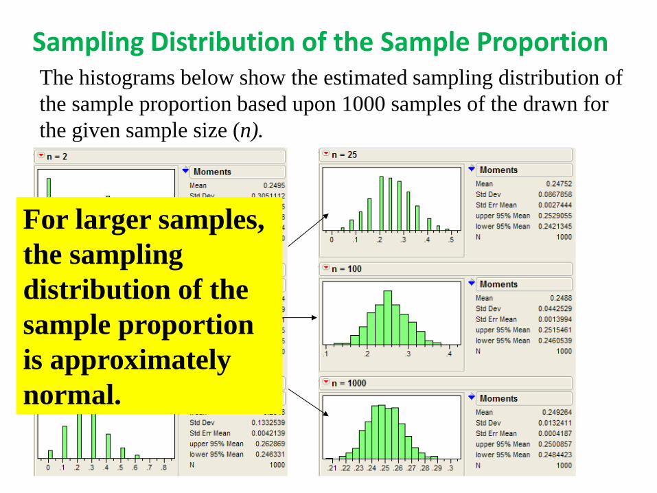
Sampling Distribution of the Sample Proportion The histograms below show the estimated sampling distribution of

the sample proportion based upon 1000 samples of the drawn for

the given sample size (n).

For larger samples,

the sampling

distribution of the

sample proportion

is approximately

normal.

Sampling Distribution of the Sample Proportion

Sampling Distribution of p̂

1. Provided n is “sufficiently large”, the sampling

distribution is normal, generally

2. The mean of the sampling distribution is

p = true population proportion

3. Standard deviation of the sampling distribution or the

standard error of sample proportion is given by:

5)1( and 5 pnnp

n

pppSE

)1()ˆ(

n

pppNp

)1(,~ˆ :Notation

Implications for Inference (n “large”)

CI for Population Proportion (p)

n

)p̂-(1p̂ value)-z(ˆ p

z-values from standard normal Distribution

Confidence z-value

90% 1.645 95% 1.960 99% 2.575

Confidence Interval for Estimating a Population Proportion

ˆ ˆp E p p E

p

p̂ E

ˆ ˆ( , )p E p E

2

ˆ ˆpqE z

n

Where E is the margin of error for proportion. It is given by

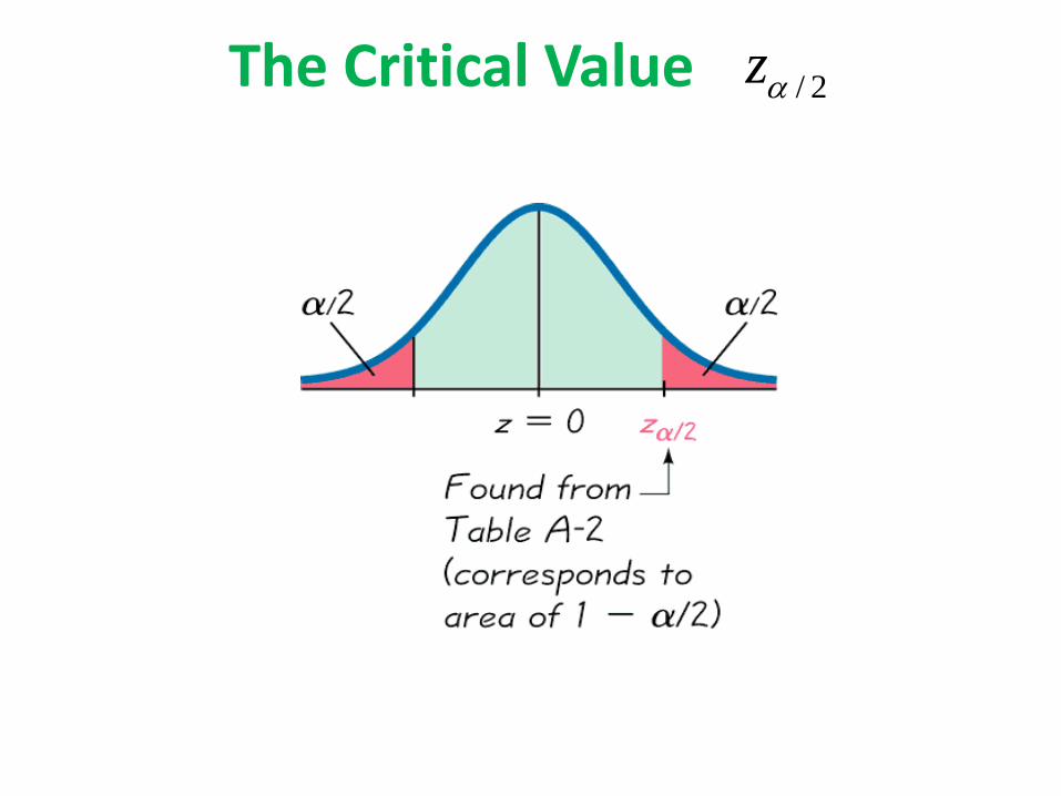
The Critical Value / 2z

Finding for a 95% Confidence Level

Critical Values

/ 2z

5%

/ 2 2.5% .025

/ 2z/ 2z

Use Table A-2 to find a z score of 1.96

Finding for a 95% Confidence Level - cont

/ 2z

0.05

/ 2 1.96z

= population proportion

Confidence Interval for Estimating a Population Proportion

= sample proportion

= number of sample values

= margin of error

= z score separating an area of in the right tail of the standard normal distribution

p

p

p̂

n

E

/ 2z / 2

1. Verify that the required assumptions are satisfied. (The sample is a simple random sample, the conditions for the binomial distribution are satisfied, and the normal distribution can be used to approximate the distribution of sample proportions because , and are both satisfied.)

2. Refer to Table A-2 and find the critical value that corresponds to the desired confidence level.

3. Evaluate the margin of error

4. Using the value of the calculated margin of error, and the value of the sample proportion, , find the values of and . Substitute those values in the general format for the confidence interval:

Procedure for Constructing a Confidence Interval for

2ˆ ˆE z pq n

p

5np 5nq

/ 2z

Ep̂ p̂ E p̂ E

ˆ ˆp E p p E

5. Round the resulting confidence interval limits to three significant digits.

Example

a. Find the margin of error that corresponds to a 95% confidence level.

b. Find the 95% confidence interval estimate of the population proportion .

c. Based on the results, can we safely conclude that the majority of adults believe in global warming?

d. Assuming that you are a newspaper reporter, write a brief statement that accurately describes the results and includes all of the relevant information.

In a Pew Research Center poll of 1501 randomly selected U.S.

adults showed that 70% of the respondents believe in global

warming. The sample results are n = 1501, and ˆ 0.70p

pE

Solution: Requirement check: simple random sample; fixed number of trials, 1501; trials are independent; two categories of outcomes (believes or does not); probability remains constant. Note: number of successes and failures are both at least 5.

b) The 95% confidence interval:

0.70 0.023183 0.70 0.023183p

0.677 0.723p

ˆ ˆp E p p E

2

0.70 0.30ˆ ˆ1.96

1501

0.023183

pqE z

n

E

a) Use the formula to find the margin of error.

c) Based on the confidence interval obtained in part (b), it does appear that the proportion of adults who believe in global warming is greater than 0.5 (or 50%), so we can safely conclude that the majority of adults believe in global warming. Because the limits of 0.677 and 0.723 are likely to contain the true population proportion, it appears that the population proportion is a value greater than 0.5.

d) Here is one statement that summarizes the results: 70% of United States adults believe that the earth is getting warmer. That percentage is based on a Pew Research Center poll of 1501 randomly selected adults in the United States. In theory, in 95% of such polls, the percentage should differ by no more than 2.3 percentage points in either direction from the percentage that would be found by interviewing all adults in the United States.

Determining Sample Size

(solve for n by algebra)

2

ˆ ˆpqE z

n

2

2

2

ˆ ˆ( )z pqn

E

Sample Size for Estimating Proportion

When an estimate of is known:

When no estimate of is known:

2

2

2

ˆ ˆ( )z pqn

E

pp̂

2

2

2

( ) 0.25zn

E

p̂

𝒏 =(𝒁𝜶

𝟐 )𝟐. σ𝟐

𝑬𝟐

If 𝝈 is given then we use the formula

Use the given information to find the minimum sample size required to estimate an unknown population mean μ. Question: How many women must be randomly selected to estimate the mean weight of women in one age group. We want 90% confidence that the sample mean is within 3.5 lb of the population mean, and the population standard deviation is known to be 20 lb. Solution: 𝒁𝜶

𝟐 = 𝟏. 𝟔𝟒𝟓, 𝝈 = 𝟐𝟎, 𝐚𝐧𝐝 𝐭𝐡𝐞 𝐞𝐫𝐫𝐨𝐫 𝐄 = 𝟑. 𝟓.

So using the formula, 𝒏 =

(𝒁𝜶𝟐 )𝟐. σ𝟐

𝑬𝟐

=(𝟏. 𝟔𝟒𝟓)𝟐. (𝟐𝟎)𝟐

(𝟑. 𝟓)𝟐

= 88.36

Hence 89 women should be selected.

Example Q. Assume that a manager for E-Bay wants to determine the current

percentage of U.S. adults who now use the Internet. How many adults must be surveyed in order to be 95% confident that the sample percentage is in error by no more than 3% points? a. In 2006, 73% of adults used the Internet. b. No known possible value of the proportion.

Solution: (a)

2

ˆ ˆ ˆ0.73 and 1 0.27

0.05 so 1.96

0.03

p q p

z

E

2

2

2

2

2

ˆ ˆ

1.96 0.73 0.27

0.03

841.3104

842

z pqn

E

To be 95% confident that our sample percentage is within three percentage points of the true percentage for all adults, we should obtain a simple random sample of 842 adults.

(b) Use

To be 95% confident that our sample percentage is within three percentage points of the true percentage for all adults, we should obtain a simple random sample of 1068 adults.

20.05 so 1.96

0.03

z

E

2

2

2

2

2

0.25

1.96 0.25

0.03

1067.1111

1068

zn

E

Interval Estimation and sample size of a Population Proportion

In a current election campaign,

PSI has just found that 220

registered voters, out of 500

contacted, favor a particular

candidate.

(a) PSI wants to develop a 95% confidence interval estimate for the proportion of the population of registered voters that favor the candidate.

(b) Suppose that PSI would like a .99 probability that the sample proportion is within + .03 of the population

proportion. How large a sample size is needed to meet the required

precision?

Example: Political Science, Inc.

p zp p

n

/

( )2

1

where: n = 500, = 220/500 = .44, z/2 = 1.96 p

Solution

PSI is 95% confident that the proportion of all voters

that favor the candidate is between .3965 and .4835.

.44(1 .44).44 1.96

500

= .44 + .0435

/2

(1 ).03

p pz

n

At 99% confidence, z.005 = 2.576. Recall that = .44. p2 2

/2

2 2

( ) (1 ) (2.576) (.44)(.56) 1817

(.03)

z p pn

E

A sample of size 1817 is needed to reach a desired precision of + .03 at 99% confidence.

(a)

(b)

Note: We used .44 as the best estimate of p in the

preceding expression. If no information is available

about p, then .5 is often assumed because it provides

the highest possible sample size. If we had used

p = .5, the recommended n would have been 1843.

Sample Size for an Interval Estimate of a Population Proportion

Estimating a Population Mean:

Not Known

With unknown, we use the Student t

distribution assuming that the relevant

requirements are satisfied.

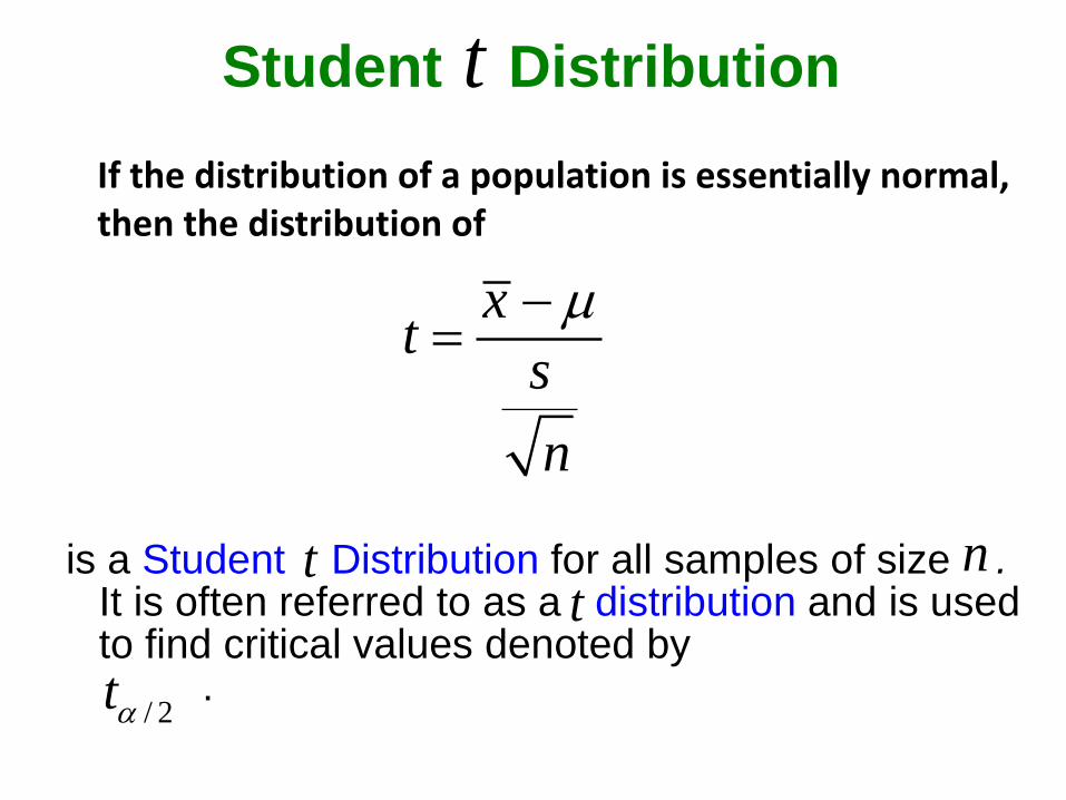
If the distribution of a population is essentially normal, then the distribution of

is a Student Distribution for all samples of size . It is often referred to as a distribution and is used to find critical values denoted by .

Student Distribution t

xt

s

n

tt n

/ 2t

degrees of freedom = n – 1

in this section.

Definition

The number of degrees of freedom for a collection

of sample data is the number of sample values

that can vary after certain restrictions have been

imposed on all data values. The degree of

freedom is often abbreviated df.

Margin of Error for Estimate of (With Not Known)

where has n – 1 degrees of freedom.

Table A-3 lists values for

E

/ 2t

/ 2t

/ 2

sE t

n

= critical t value separating an area of in the right tail

of the t distribution

/ 2t / 2

where

found in Table A-3

Confidence Interval for the Estimate of (With Not Known)

df = n – 1

/ 2t

/ 2

sE t

n

x E x E

2. Using n – 1 degrees of freedom, refer to Table A-3 or use technology to find the critical value that corresponds to the desired confidence level.

Procedure for Constructing a Confidence Interval for (With Unknown)

1. Verify that the requirements are satisfied.

3. Evaluate the margin of error

4. Find the values of Substitute those values in the general format for the confidence interval:

5. Round the resulting confidence interval limits.

and .x E x E

/ 2t

/ 2

sE t

n

x E x E

Example

A common claim is that garlic lowers cholesterol levels. In

a test of the effectiveness of garlic, 49 subjects were

treated with doses of raw garlic, and their cholesterol

levels were measured before and after the treatment. The

changes in their levels of LDL cholesterol (in mg/dL) have

a mean of 0.4 and a standard deviation of 21.0. Use the

sample statistics of

to construct a 95% confidence

interval estimate of the mean net change in LDL

cholesterol after the garlic treatment. What does the

confidence interval suggest about the effectiveness of

garlic in reducing LDL cholesterol?

49, 0.4 21.0n x and s

Solution Requirements are satisfied:

simple random sample and

.

2

21.02.009 6.027

49E t

n

95% implies .

With n = 49, the df = 49 – 1 = 48

Closest df is 50, two tails, so

Using

the margin of error is:

/ 2 2.009t

49 ( . ., 30)n i e n

0.05

/ 2 2.009, 21.0 49t s and n

Table A-3 T Distribution

α

Degrees

of

Freedom

.005

(one tail)

.01

(two tail)

.01

(one tail)

.02

(two tail)

.025

(one tail)

.05

(two tail)

.05

(one tail)

.10

(two tail)

.10

(one tail)

.20

(two tail)

.25

(one tail)

.50

(two tail)

1 63.657 31.821 12.706 6.314 3.078 1.000

2 9.925 6.965 4.303 2.920 1.886 .816

3 5.841 4.541 3.182 2.353 1.638 .765

4 4.604 3.747 2.776 2.132 1.533 .741

5 4.032 3.365 2.571 2.015 1.476 .727

6 3.707 3.143 2.447 1.943 1.440 .718

7 3.500 2.998 2.365 1.895 1.415 .711

8 3.355 2.896 2.306 1.860 1.397 .706

9 3.250 2.821 2.262 1.833 1.383 .703

7

3.500 2.998 2.365 1.895 1.415 .711

8 3.355 2.896 2.306 1.860 1.397 .706

9 3.250 2.821 2.262 1.833 1.383 .703

10 3.169 2.764 2.228 1.812 1.372 .700

11 3.106 2.718 2.201 1.796 1.363 .697

39 2.708 2.426 2.023 1.685 1.304 .681

40 2.704 2.423 2.021 1.684 1.303 .681

50 6.678 2.403 2.009 1.676 1.299 .679

Construct the confidence

interval:

0.4, 6.027x E

We are 95% confident that the limits of –5.6 and 6.4 actually

do contain the value of , the mean of the changes in LDL

cholesterol for the population. Because the confidence

interval limits contain the value of 0, it is very possible that

the mean of the changes in LDL cholesterol is equal to 0,

suggesting that the garlic treatment did not affect the LDL

cholesterol levels. It does not appear that the garlic treatment

is effective in lowering LDL cholesterol.

0.4 6.027 0.4 6.027

5.6 6.4

x E x E

Important Properties of the Student Distribution

1. The Student distribution is different for different sample sizes (see the following slide, for the cases n = 3 and n = 12).

2. The Student distribution has the same general symmetric bell shape as the standard normal distribution but it reflects the greater variability (with wider distributions) that is expected with small samples.

3. The Student distribution has a mean of (just as the standard normal distribution has a mean of ).

4. The standard deviation of the Student distribution varies with the sample size and is greater than 1 (unlike the standard normal distribution, which has a ).

5. As the sample size gets larger, the Student distribution gets closer to the normal distribution.

tt

t

t 0t 0z

t

1

n t

Properties of the t Distribution • mound-shaped

• perfectly symmetric about t=0

• more variable than z (the standard normal distribution)

• affected by the sample size n (as n increases s

becomes a better approximation for σ)

• n-1 is the degrees of freedom (d.f.) associated

with the t statistic

Student Distributions for n = 3 and n = 12

t

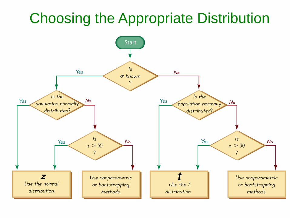
Choosing the Appropriate Distribution

Choosing the Appropriate Distribution

Use the normal (z) distribution

known and normally distributed population or known and

Use t distribution not known and normally distributed population or not known and

Use a nonparametric method or bootstrapping

Population is not normally distributed and

30n

30n

30n

Finding the Point Estimate and from a Confidence Interval

Margin of Error:

= (upper confidence limit) — (lower confidence limit)

2

Point estimate of :

= (upper confidence limit) + (lower confidence limit)

2

E

p̂

p̂

E