Chapter 8Centrality in Networks: Finding the MostImportant Nodes
Sergio Gómez
Abstract Real networks are heterogeneous structures, with edges unevenly dis-tributed among nodes, presenting community structure, motifs, transitivity, richclubs, and other kinds of topological patterns. Consequently, the roles played bynodes in a network can differ greatly. For example, some nodes may be connectorsbetween parts of the network, others may be central or peripheral, etc. The objectiveof this chapter is to describe how we can find the most important nodes in networks.The idea is to define a centrality measure for each node in the network, sort thenodes according to their centralities, and fix our attention to the first ranked nodes,which can be considered as the most relevant ones with respect to this centralitymeasure.
Keywords Centrality · Betweenness centrality · Closeness centrality · Degreecentrality · Eigenvector centrality · Hubs and authorities centrality · Katzcentrality · PageRank centrality · Random walk centrality · Versatility centrality
8.1 Introduction
Datasets in business and consumer analytics can be frequently represented in theform of networks, in which the nodes represent any kind of item, e.g., products,consumers, brands, firms, etc., while the links represent relationships betweenthem. For example, in co-purchasing networks, the links could account for pairs ofproducts bought together, whereas in international trade networks the edges couldrepresent the amount of a product which is exported from one country to another.The possibilities are infinite, and the extraction of information from these networks
S. Gómez (�)Universitat Rovira i Virgili, Tarragona, Spaine-mail: [email protected]
is the object of study in several fields, from complex networks and complex systemsto data science, among others. Here we aim at finding the most important nodes ina network, which could be crucial in many business applications.
The importance of a node in a complex network depends on the structuralcharacteristic or dynamic behaviour we could be interested in. Consequently, theliterature is full of different definitions, all of them perfectly meaningful underspecific set-ups. Our objective is to explain the rationale behind the most widelyused centrality measures, to be able to decide which one is the more adequatefor our needs. Most of them are easy to describe and understand, some are alsoeasy to calculate with the appropriate tools, while others represent a computationalchallenge which requires the use of complex algorithms which are not easy toimplement. Fortunately, several software applications and packages exist whichsimplify the finding of the centralities of the nodes in complex networks.
The structure of this section is as follows. First, after this short introduction,we will introduce in Sect. 8.2 the mathematical notation to represent complexnetworks, which is needed to formalize the different network centralities. Next,we will describe in Sect. 8.3 the most relevant approaches and definitions for thecentralities of the nodes in unweighted networks, which represent the core of thischapter of the book. Then, we will show in Sects. 8.4 and 8.5 how it is possible toextend the centralities to cope with two different types of more general networks:weighted networks and multilayer networks. This will be followed in Sect. 8.6 bythe calculation of the most central nodes for several synthetic and real networks.In Sect. 8.7 we enumerate the main software tools to calculate the centrality innetworks, and we conclude in Sect. 8.8 with a summary of centrality in networksand their applications.
8.2 Mathematical Notation
The main mathematical object in the study of complex networks is the adjacencymatrix A = (aij ), which encodes the full topology of the network or graph: aij = 1if there is an edge from node i to node j , and aij = 0 otherwise.1 We suppose thenetwork has N nodes, thus i, j ∈ {1, . . . , N}. If the direction of the links is notimportant, the network is called undirected, and the adjacency matrix is symmetric,A = AT , where AT denotes the transpose of matrix A. For undirected networks, thedegree ki of a node is its number of neighbours, and is calculated as
1In some texts the adjacency matrix is defined in the opposite direction, i.e., aij is used to encodean edge from node j to node i, for example, in [44]. This is an important issue to care about whendealing with directed networks.
8 Centrality in Networks: Finding the Most Important Nodes 403
ki =N∑
j=1
aij . (8.1)
Directed networks require the distinction between the links that arrive to a node andthose that depart from it, therefore it is convenient to distinguish between the outputand input degrees:
kouti =
N∑
j=1
aij , (8.2)
kini =
N∑
j=1
aji . (8.3)
Of course, if the network is undirected, kouti = kin
i = ki . We will try to describethe centrality measures in the general case of directed networks, since undirectednetworks can be considered just as particular cases. However, there are definitionsof centrality which do not make sense or cannot be calculated for certain kinds ofnetworks, thus we will explicitly explain the applicability of each centrality type.We will also suppose there are no self-loops in the network, thus all the diagonalelements of the adjacency matrix are zero, aii = 0. The number of edges iscalculated by just taking the sum of all the components of the adjacency matrix:
2L =N∑
i=1
N∑
j=1
aij . (8.4)
The number of edges is L for undirected networks, but 2L for directed ones. Thereason is that the adjacency matrix of undirected networks counts every edge twice,aij = aji = 1.
8.3 Centrality in Networks
The list of centralities we are going to describe is the following:
• Degree centrality• Closeness centrality• Betweenness centrality• Eigenvector centrality• Katz centrality• Hubs and authorities centrality• PageRank centrality• Random walk centralities.
A more complete review on centrality, covering many other definitions [40], algo-rithms [36], and several advanced concepts [41] (personalization, axiomatization,stability, and sensitivity) can be found in [17].
8.3.1 Degree Centrality
The first and simplest proposal of a centrality measure for the nodes in a network isthe degree,
C(deg)i = ki . (8.5)
This is a concept which was developed in the context of social networks a long timeago [30, 57]. The idea was that a person having many direct connections to otherpeople must be central with respect to the communication between them, acquiringa sense of being in the mainstream of information. On the contrary, people with alow degree could miss most of the information flowing in the network, thus playinga residual role.
Nodes with high degree, clearly above the average in the network, are calledhubs. The discovery that many real-world networks have power-law degree distri-butions [4], with only a few hubs collecting a great proportion of the overall linksin the network, was in fact one of the cornerstones in the development of the actualtheory of complex networks.
Sometimes it is useful to normalize the centralities considering their maximumvalue, which for the degree equals N − 1, thus
C(deg,norm)i = ki
N − 1. (8.6)
However, normalization is usually not needed, since what matters is the rank of thenodes after sorting them according to the selected centrality measure (which doesnot change with normalization).
Several additional centrality measures were defined as variants of the degree (see,e.g., [32, 48, 52, 57]), but they have become outdated, so we just skip them.
The degree is a simple and effective centrality measure for undirected networks,but not for directed ones, in which we have to distinguish between incoming andoutgoing links. A possible approach could be to take as centrality the sum, kin
i +kouti ,
i.e., the total number of connections discarding their directionality, or the average ofboth input and output degrees, (kin
i +kouti )/2; the average is more convenient because
it coincides with the degree when applied to undirected networks:
8 Centrality in Networks: Finding the Most Important Nodes 405
Another alternative consists in defining two degree centralities, one for theincoming and the other for the outgoing links, since they measure different things: anode with high input degree centrality represents a node which is in good position toreceive information, while large output degree centralities correspond to importantsources of information:
C(deg,out)i = kout
i , (8.8)
C(deg,in)i = kin
i , (8.9)
Now, it becomes clear why the importance of a node is closely related to theprocess or property we are interested in, since even degree centrality admits severaldiverging interpretations in directed networks.
8.3.2 Closeness Centrality
If you have items distributed within a circle, its centre has the property that all theitems are at a distance equal or smaller than the radius, while other positions may beas much as twice that distance. This suggests that a measure of centrality in networkscould consider the distances to the rest of the nodes, and thus central nodes wouldbe close to all of them. The advantage of being central in this way comes from thepossibility of sending or broadcasting information, being sure the time needed toreach the whole network is as short as possible. Closeness centrality is based on thisidea: for each node, you calculate the distance to all the other vertices in the network,and define a centrality in which shorter distances imply higher closeness centrality,and vice versa. There are several ways of expressing this concept mathematically.First, let us call dij the distance between nodes i and j . The distance in a graph isdefined as the minimum number of hops (following links) needed to move from onenode to another, or, in other words, the length of the shortest path between them.Then, the closeness centrality [9, 54] reads
The difference between using N − 1 or N is irrelevant for the ranking of the nodes.The N − 1 makes sense since the distance from a node to itself is always zero,dii = 0, but the N provides simpler expressions for certain analytic derivations.
Here we are supposing the network is connected (strongly connected if directed),otherwise some of the distances are infinity and the closeness centrality of all nodesbecomes zero. To avoid these infinities, a simple heuristic consists of replacingeach infinite distance by N , i.e., a value larger than all the finite distances. Analternative definition which maintains the infinities and works even if the network isnot connected is found by just swapping the reciprocal and sum operations [25]:
C(clos2)i = 1
N − 1
N∑
j=1j =i
1
dij
, (8.13)
where, by convenience, dij = ∞ if there is no path between i and j , i.e., 1/dij =0. The term 1/dii is explicitly excluded from the sum to avoid the correspondinginfinity. Equation (8.13) may be viewed as a centrality based on the harmonic meanof the distances, and has the advantage that most of the contribution comes from thedistances to the closer nodes.
The calculation of all distances in general unweighted graphs requires a breadth-first search (BFS), which takes O(L + N) time, for each of the nodes, thusrepresenting a total cost O(NL+N2). For sparse networks we have that L ∼ O(N),thus the total cost is reduced to O(N2). For the weighted networks that we willcover in Sect. 8.4, BFS must be substituted with Dijkstra’s algorithm, with a costO(L+ N log N), thus raising the total cost of calculating the closeness centralitiesto O(NL + N2 log N) in general networks, and to O(N2 log N) for sparse ones.Alternatively, the Floyd-Warshall algorithm finds all the shortest paths with anO(N3) upper bound [27], which may be useful to reduce part of the overhead (butnot the total cost) in the application of multiple Dijkstra’s algorithms.
Likewise to degree centrality, closeness centrality also admits output and inputversions for directed networks, depending on whether the distances are computedfrom or to the reference node, respectively. Note that distances are not symmetricin directed networks. Since we already have several definitions for the closenesscentrality, the addition of input and output closeness centralities multiplies theoptions. This is important to be aware of, since different software may choose andimplement centralities in distinctive ways, thus being not exactly comparable.
8 Centrality in Networks: Finding the Most Important Nodes 407
8.3.3 Betweenness Centrality
Betweenness is another of the traditional centrality measures developed in the studysocial science. Here we fix our attention in the nodes which are crossed when youfollow shortest paths. A node which falls in the communication paths between manypairs of nodes plays an important role, since it can control the flow of information.Formally, the standard measure for this property is called betweenness centrality [2,29], and is defined as
C(betw)i = 1
(N − 1)(N − 2)
N∑
s,d=1s =d =i
σsd(i)
σsd
. (8.14)
The sum covers all source/target pairs of nodes, excluding node i, σsd representsthe number of shortest paths from source node s to destination node d, and σsd(i)
is the number of those paths that include node i. In other words, the betweenness isthe average fraction of paths that cross a node. This expression of the betweennessmeasure is valid for both directed and undirected networks, and includes the optionalnormalization factor. If there are no paths between the origin s and the destination d
(disconnected graph), then σsd = 0 and it becomes necessary to define σsd(i)/σsd =0. An example of a node with high betweenness would be a node which is a bridgebetween two disconnected parts of the network: to go from one part of the networkto the other you are forced to cross the bridge, no matter if this node has just afew links. Betweenness naturally appears in communication dynamics on top ofcomplex networks, e.g., it can be shown that the onset of congestion in a simplemodel of routing is related to the maximum betweenness of the system [34].
As we have explained for the closeness centrality, the calculation of shortestpaths represents a costly task. Fortunately, we may apply the Brandes’ algorithmfor betweenness centrality, with a cost O(NL + N2 log N), which is reduced toO(NL+N2) for the unweighted networks we have considered so far [16].
Some variations on the definition of betweenness exist; the most remarkable onebeing the possibility of including node i as both source s and destination d [44],which we have forbidden in our previous definition. The decision of including ornot the end-points of the paths when calculating the betweenness depends on theparticular dynamics you may be interested in. For example, in routing dynamics inwhich a queue is attached to each node, it is possible to decide between putting thecreated packets in the queue of the source node [60], or skipping this queue andenqueuing them directly to the first neighbour in the path [34]. Both alternatives areacceptable, but they lead to slightly different values of the betweenness. Anothervariant of betweenness is the one which calculates the number of shortest paths atthe level of edges, thus defining a link betweenness, the natural extension to links ofthe vertex betweenness. We are not going to consider link centralities in the rest ofthis chapter, but it may be useful for the reader to know of their existence and oneof their paradigmatic examples.
All the previous centrality measures take into account the topological position ofnodes in the network, but not the importance of the nodes themselves. It could bedesirable, for example, that a node be considered as important if its neighboursare also important. This leads to a recursive definition of centrality, in which thecentrality of a node depends on the centralities of the neighbours, which are alsounknown. Fortunately, it is possible to write self-consistent equations which caneasily be solved using linear algebra techniques. The simplest of this kind ofapproach consists of defining the centrality of a node as proportional to the sum ofthe centralities of the neighbours, so as the larger the importance of the neighbours,the more central the node is [13–15]. In mathematical terms,
λC(eig)i =
N∑
j=1
ajiC(eig)j , (8.15)
where λ is the proportionality constant. The aji term emphasizes that node i receivesthe contribution to centrality from its neighbours through the incoming links. Forexample, in the World Wide Web network, building a website with many links toimportant sites is easy to build and has no cost, so it gives no information at all.However, receiving hyperlinks from relevant sites is a good indicator of quality, andcan be used to measure the centrality of the website.
Equation (8.15) is expressed in matrix form as
AT C(eig) = λC(eig) , (8.16)
which means the vector of centralities C(eig) is an eigenvector of AT (or equivalently,a left-eigenvector of A) with eigenvalue λ. Since the components of the adjacencymatrix are all non-negative, we can apply the Perron-Frobenius theorem [31, 51],which ensures that, if the matrix is irreducible, there exists a unique solution ofEq. (8.16) in which all the centralities C
(eig)i are positive (up to positive common
factors), and which corresponds to the largest eigenvalue λ > 0. The matrix isirreducible if the graph is strongly connected (or simply connected, if the networkis undirected). For directed networks this condition is difficult to be fulfilled, thuseigenvector centrality is basically used only for undirected networks. Some variantsof the eigenvector centrality, such as Katz, HITS, or PageRank, are more adequatefor directed networks.
The calculation of the eigenvector centrality can easily be performed by poweriteration: initialize all the centralities to one (or to a random positive vector),multiply by AT , normalize the vector, and repeat the multiplication-normalizationsteps until convergence. Common normalizations used are those in which the sumof all centralities are either 1 or N . Again, the normalization does not affect theranking of the nodes, thus any choice is equally acceptable. The cost of power
8 Centrality in Networks: Finding the Most Important Nodes 409
iteration in O(Lr) for general graphs, and O(Nr) for sparse ones, where r is thenumber of iterations needed until convergence to the desired precision. Convergenceis guaranteed if the adjacency matrix has a non-degenerate maximum (in magnitude)eigenvalue, and the initial vector has a non-zero component in the direction ofthe leading eigenvector. The convergence is geometric with ratio |λ2/λ1|, i.e.,the quotient between the second and the first eigenvalues, thus it depends on thestructure of the whole network and it is impossible to predict the value of r without acomputation which may take longer than the calculation of the eigenvector centralityitself.
8.3.5 Katz Centrality
Katz centrality is a proposal that lays between degree and eigenvector centrality. Itwas introduced as a way of generalizing the degree centrality, taking into accountnot only the immediate neighbours but also the nodes reachable in larger numberof steps [37]. Since you want that the closer the nodes, the larger their influence,a decay parameter α < 1 is introduced to weight the contributions of nodes atincreasing path lengths. It is defined in this way:
C(katz)i =
∞∑
k=1
N∑
j=1
αk(Ak)ji . (8.17)
The power matrix Ak accounts for the number of paths of length k between everypair of nodes, e.g., (A3)ji = ∑
r
∑s ajrarsasi , where the paths start at node j ,
then go to node r , next to s, and finally arrive to i, for all possible values of theintermediate nodes r and s. Denoting I the identity matrix of order N , and 1 thevector of length N with all components equal to 1, we can write
Equations (8.19) and (8.20) are closely related to the eigenvector centralityEqs. (8.16) and (8.15), respectively. Basically, the Katz centrality of a node is relatedto the centralities of the incoming neighbours, likewise eigenvector centrality, butwith the addition of one unit per neighbour. This means all nodes have a minimumlevel of centrality, different from zero, which helps to avoid the problems ofeigenvector centrality with non-strongly connected components. Of course, the α
parameter has to be small enough to ensure the convergence of Eq. (8.17) and of theiteration process. It can be shown that proper values of the parameter must be in theinterval 0 < α < 1/λ, where λ is the maximum eigenvalue of the adjacency matrixA.
Katz centrality can be extended by replacing the vector 1 by any other set ofconstants:
C(katz2) = αAT C(katz2) + β , (8.21)
This is useful to allow each node i to have a minimum centrality βi , which could beset even from external information of the nodes, unrelated to the network structure.When α approaches zero most of the contribution to the Katz centrality comesfrom the constant term β, while α values close to its upper bound 1/λ give thedominant role to the eigenvector term. In practice, most of the authors use values ofthe parameter near the upper bound.
Although Katz centrality could be computed with a matrix inversion usingEq. (8.18), it is more efficient to directly solve Eqs. (8.19) or (8.21) by iterationuntil convergence, in a similar way as for the eigenvector centrality, and equivalentcost O(Lr) for general complex networks.
8.3.6 Hubs and Authorities Centrality
In directed networks, nodes can have very different roles if we consider onlythe input or output links. The idea of the hyperlink-induced topic search (HITS)approach, also known as hubs and authorities’ algorithm [39], is to assign to eachnode a couple of scores: a hub centrality, which takes into account the role of thenode in sending links, and an authority centrality, measuring the capacity of thenode to receive links. Following the same approach that eigenvector centrality, theimportance as authority depends on the relevance of the hubs that send the incominglinks, and the other way around, important hubs give more weight as authorities tothe receiver nodes. Denoting C
8 Centrality in Networks: Finding the Most Important Nodes 411
C(hub)i = β
N∑
j=1
aijC(auth)j . (8.23)
In matrix form,
C(auth) = αAT C(hub) , (8.24)
C(hub) = βAC(auth) , (8.25)
which can be combined to form two decoupled equations:
AT AC(auth) = γ C(auth) , (8.26)
AAT C(hub) = γ C(hub) , (8.27)
where γ = (αβ)−1. Applying the Perron-Frobenius theorem as for the eigenvectorcentrality, and realizing that matrices AT A and AAT are symmetric, then theauthorities and hubs centralities are given by the leading eigenvector of theirrespective matrices. Moreover, it can be shown that the eigenvalues of AT A andAAT are exactly the same, thus the two equations are consistent and γ is themaximum eigenvalue of any of them. Additionally, multiplying both sides of thefirst equation by A and of the second equation by AT , we get
AAT (AC(auth)) = γ (AC(auth)) , (8.28)
AT A(AT C(hub)) = γ (AT C(hub)) , (8.29)
which means that hubs and authorities centralities are related in the following way:
C(auth) = AT C(hub) , (8.30)
C(hub) = AC(auth) . (8.31)
This framework was designed to rank web pages, but is perfectly valid for allkinds of directed networks, e.g., citations or trade networks. When the networkis undirected the distinction between hubs and authorities disappears, and theircentralities coincide with those obtained by eigenvector centrality.
The most effective way of calculating these centralities is by iteration ofEqs. (8.30) and (8.31), with a normalization after each step, and a total cost equiv-alent to eigenvector and Katz centralities. The result is both hubs and authoritiescentralities at the same time, and it skips the excessive time consuming matrixmultiplications in Eqs. (8.28) and (8.29).
PageRank has become a notorious centrality measure since it lays at the core of theGoogle search engine. When you make a search query, the PageRank score of eachweb page is used to sort the results, which are then presented to the user. Of course,PageRank is in fact used in conjunction with other heuristics and criteria, but at leastit provides a good starting point.
The rationale behind PageRank is similar to eigenvector centrality, but with arelevant distinction: when a node receives a link from an important source, it isnot the same if that site has many links or just a few. If the number is large,the contribution is diluted, and should be penalized. Thus, it seems reasonable tonormalize the score of a node by its number of outgoing links, before adding itto the score of the receiver. The full equation for the PageRank centrality is thefollowing [19]:
C(pr)i = α
N∑
j=1
aji
C(pr)j
koutj
+ 1− α
N. (8.32)
The constant term plays an equivalent role as in Katz centrality, ensuring the equa-tion has a unique and non-trivial solution for directed networks, while parameterα, known as the dumping factor, controls the fraction of contribution betweenthe eigenvector and constant terms. Note that PageRank is already normalized,∑
i C(pr)i = 1, as can be easily checked by summing both sides of Eq. (8.32) for
all the nodes i. For nodes with no outbound links, koutj = 0, but the numerator is
also zero, thus a simple solution is to replace koutj by max(kout
j , 1); otherwise, theterms 0/0 are just supposed to be 0.
We may also write Eq. (8.32) in matrix form:
C(pr) = αAT D−1C(pr) + 1− α
N1 , (8.33)
where D is the diagonal matrix with elements Dii = max(kouti , 1). In this way, the
solution is given by:
C(pr) = 1− α
N(I − αAT D−1)−11
= 1− α
ND(D − αAT )−11 . (8.34)
Anyhow, the common way of solving Eq. (8.32) is by iteration, as explained for theprevious eigenvector, Katz and HITS centralities. The dumping factor was set bythe authors to α = 0.85, but this is a quite arbitrary selection which can be tuned asdesired.
8 Centrality in Networks: Finding the Most Important Nodes 413
8.3.8 Random Walk Centralities
Looking at Eq. (8.32) for the PageRank, a new interpretation comes out when werealize that
Pij = aij
kouti
(8.35)
represents the probability that a random walker follows a link from node i to nodej [43, 49, 61]. Matrix P , which may be written as
P = D−1A , (8.36)
is right stochastic, since∑
j Pij = 1 for all rows i, i.e., P 1 = 1. The probabilityπi that a random walk is found in node i is obtained by solving the eigenvectorequation
P T π = π . (8.37)
Using P , the PageRank equation becomes
C(pr) = αP T C(pr) + 1− α
N1 . (8.38)
This equation corresponds to the dynamics of a random walker which, withprobability α, follows a random link of the current node, and with probability 1− α
jumps to a random node; this behaviour justifies why the second term is also referredto as the teleportation term, and it is necessary to escape from nodes without outputlinks. Moreover, C(pr) turns out to be the occupation probability of this randomwalker, thus providing a physical interpretation: PageRank centrality is equal to theprobability of the random walker being found at each of the nodes.
If we remove the teleportation term by setting the dumping factor to α = 1, thePageRank equation is simplified to C(pr) = P T C(pr), which has a simple solution forunweighted networks: C(pr) = k = C(deg), i.e., the PageRank becomes proportionalto the degree. In the general case of directed networks and with teleportation thissolution does not hold, but it suggests that PageRank is a kind of modified versionof the degree centrality.
We have shown so far that a random walk dynamics on complex networks givesan alternative explanation of PageRank to the one inspired by eigenvector and Katzcentrality. However, this is not the only centrality measure that can be defined usingrandom walks. In fact, random walks constitute a good proxy for the spreading ofinformation in networks, and we can take advantage of it to introduce new measuresof the importance of nodes. In particular, we are going to briefly describe random-walk closeness centrality and random-walk betweenness centrality [46].
In the definition of betweenness centrality given in Sect. 8.3.3, only nodescrossed by shortest paths are considered. This makes sense for certain dynamics,e.g., vehicles trying to reach their destination minimizing the travel distance, orservers dispatching packets using the standard Internet protocols. The same can besaid about closeness centrality, which implicitly assumes that shortest-path distancesare the way to go from one node to another. However, if we consider rumours,news, fads, or epidemics, to name a few, their spreading is more random, and forsure they do not follow shortest paths. This is where random walkers stand out, asan alternative and often better model of information spreading that can help in theintroduction of additional measures of centrality. In fact, real propagation usuallylays somewhere in-between shortest paths and random walks, the two extreme cases.
A measure of random-walk betweenness centrality requires the computation ofthe probability that a random walk crosses a certain node while travelling betweenall other pairs of nodes. This is accomplished by introducing a new transition matrixP [d] with an absorbing state at the destination node d (when the random walkerarrives to d, it is removed from the system),
P[d]ij =
{0 if i = d
Pij otherwise,(8.39)
and calculating the expected number of times the random walker crosses node i (inany number of steps) when starting at node s and before reaching the destination d,
q[d]si =
∞∑
n=0
1
kouti
[(P [d])n
]
si
=[(I − P [d])−1D−1
]
si
=[(D − A[d])−1
]
si, (8.40)
where A[d] is defined as in Eq. (8.39). The n-th power of P [d] term expresses theprobability of arriving from node s to node i in n steps, and the 1/kout
i adds thecondition of leaving that node by any of the links, thus effectively crossing node i.
Since random walkers may be trapped in parts of the network which are not reallyrelated to the paths between nodes s and d, it is essential to cancel out, for each link,the flux in opposite directions. For example, the net flux through the link (i, j) isequal to |q[d]si − q
[d]sj |, which yields a net flux at node i equal to
8 Centrality in Networks: Finding the Most Important Nodes 415
Finally, random-walk betweenness centrality is obtained by averaging the node fluxover all possible origins and destinations,
C(rwbetw)i = 1
N(N − 1)
N∑
s,d=1s =d
f(sd)i . (8.42)
In this case we have allowed node i to be in the end-points of the paths, unlikefor shortest-path betweenness, but we could restore the same semantics by settingf
(sd)s = f
(sd)d = 0 in Eq. (8.41) and normalizing the centrality by (N − 1)(N − 2)
instead of N(N − 1).The computing cost of this centrality is high due to the need of finding the inverse
of N matrices (one for each absorbing node d), all of size N × N . However, it canbe shown that the same solution can be obtained with just one matrix inversion, bychoosing an arbitrary node v (e.g., the first one), finding the corresponding inversematrix R = (D−A[v])−1, and calculating the flux of all nodes using the componentsof matrix R as
f(sd)i =
⎧⎪⎪⎨
⎪⎪⎩
1
2
N∑
j=1
aji
∣∣(rsi − rdi)− (rsj − rdj )
∣∣ if i = s, d
1 otherwise.
(8.43)
In this way, the total cost of computing the random-walk betweenness centralitybecomes O((N + L)N2), where O(N3) corresponds to the matrix inversion andO(N2L) to the calculation of the net flux of all nodes. For sparse matrices, the costis reduced to O(N3).
Random-walk closeness centrality follows the same idea: the distance betweentwo nodes s and d is replaced by the average time needed by a random walkerto reach d when starting the walk at s. This quantity receives the name of meanfirst-passage time (MFPT), and has the property of not being symmetric even forundirected networks. The MFPT in which origin and destination are the same nodeis known as mean return time. The derivation of MFPT matrix T is quite involved[44, 62], but we can give the recipe for its calculation, based on the fundamentalmatrix Z of the random walk dynamics:
Z = (I − (P − P∞))−1 , (8.44)
where P∞ = limn→∞ P n = 1πT . Then, the MFPT from node s to node d is givenby
and the random-walk closeness centrality is just defined as
C(rwclos)i = 1
hi
. (8.47)
Note that we have based the definition on the paths arriving to the node for whichwe are calculating the centrality, thus using the same choice as for the PageRankand other centralities. The cost for random-walk closeness centrality comes fromthe matrix inversion needed to find the fundamental matrix Z, thus it is O(N3).
8.4 Centrality in Weighted Networks
Weighted networks are those for which a certain value is assigned to each of theedges. The standard interpretation is that the larger the weight, the more connectedor related the nodes are. Flows, similarities, strengths of social ties, capacities,correlations, intensities, and proximities are examples of this kind of weightedrelationships. The matrix of weights wij may be seen as a generalization of theadjacency matrix, in the sense that we may consider that a null weight corresponds tothe absence of a link, and in many cases we may just replace the adjacency matrix bythe weights matrix to obtain generalizations of the unweighted concepts, centralitybeing one of them [1, 5]. Note also that the adjacency matrix is recovered if wesuppose all the weights are equal to 1. The natural generalization of the degree iscalled the strength of the node and is given by
wi =N∑
j=1
wij . (8.48)
Directed networks require the distinction between input and output strengths,
8 Centrality in Networks: Finding the Most Important Nodes 417
2w =N∑
i=1
N∑
j=1
wij . (8.51)
With these ingredients, the generalization of the degree centrality would be thestrength centrality, which could be normalized using the maximum strength. In thesame way, eigenvector, hubs and authorities, and PageRank centralities are obtainedby simple substitution of the adjacency matrix components and the degrees byweights and strengths, respectively. The Katz centrality also admits this treatmentin its interpretation as an eigenvalue problem, but it is questionable the meaning ofthe powers of the weights matrix.
For the random-walk centralities, the weights allow to have different transitionprobabilities from a node to each of its neighbours,
Pij = wij
wouti
, (8.52)
and once they are determined, the definitions of PageRank, random-walk between-ness, and random-walk closeness remain the same.
The problem arises when we want to generalize centralities based on distances,like closeness or betweenness. The first option consists in discarding the weights,something which also applies to the cases above. However, when the relationshipbetween nodes represents distances, they cannot be ignored. For example, ingeographical and transportation networks we may have the distances betweenconnected nodes available. Now, the shortest path between two nodes is not thepath with the least number of hops, but the path for which the sum of the distancesof the edges (the length of the path) is the smallest one. In these cases, the definitionof closeness and betweenness centralities does not need to be changed, but thealgorithms to calculate them require important modifications. For instance, whilea breadth-first search is enough to find the distances in unweighted networks, aDijkstra’s algorithm is necessary to cope with the distances of the edges.
8.5 Centrality in Multilayer Networks
Another important class of networks which deserves special treatment with regardto centrality is that of interconnected multilayer networks [12, 38]. In multilayernetworks the nodes are distributed in layers, with intra-layer and inter-layer linksconnecting nodes in the same and different layers, respectively. If every noderepresents a different entity, no matter in which layer it is located, it is perfectlymeaningful to calculate the centralities of the nodes as if the network were notmultilayer, i.e., disregarding the structure in layers. Alternatively, we could just findthe centralities of the nodes inside the layers, considering each layer as a separatenetwork, ignoring the inter-layer links. These procedures lead to two centralities per
node, one global and the other local to the layer. Thus, a node can be at the sametime very central in a layer, but not so important for the whole multilayer network.
In interconnected multilayer networks the same node may be present in severallayers at the same time, and this fact affects the definition of centrality itself. If onenode has a different centrality in each layer, how do we have to aggregate them toproduce a single centrality for the node? There have been several proposals of waysto define eigenvector centralities [35, 58] and PageRank [8] for multiplex networks,which are the particular case of multilayer interconnected networks in which inter-layer links only connect instances of the same node in different layers, but notdifferent nodes. A more general framework makes use of the tensorial formulationof multilayer networks [23], which has allowed a grounded development of theextension of centrality measures to general multilayer networks [24, 59]. Theremarkable finding is that centrality in interconnected multilayer networks revealsthe most versatile nodes, in the sense that the highest centrality (versatility) isassigned to nodes which are not necessarily very central in any layer but whichare fundamental for the cohesiveness and integration of the whole structure [24].
We are not going to develop all the theory of centrality (versatility) for multilayernetworks, but it is easy to show the main ideas with eigenvector centrality. First, thereplacement of the adjacency matrix for multilayer networks is the adjacency tensorMiα
jβ , representing the links between nodes i in layer α and nodes j in layer β. Theeigentensor equation becomes:
N∑
i=1
U∑
α=1
MiαjβC
(eigvers)iα = λC
(eigvers)jβ , (8.53)
where U is the number of layers. After solving this equation for the largesteigenvalue, the final eigenvector centrality (versatility) is obtained by summing upthe contributions at each layer:
C(eigvers)j =
U∑
β=1
C(eigvers)jβ . (8.54)
Note that Eq. (8.53) takes into account the complete structure of the multilayernetwork, unlike some approaches in which layers are analysed as isolated layers,thus losing the information of the inter-layer connectivity.
In a similar way, centralities based on distances or random walkers make useof the full structure of the network, but at the same time the multiplicity of thenodes in the different layers poses restrictions on the paths. For example, althoughpaths may change layer crossing inter-layer links, it is natural to consider thatshortest paths from an origin to a destination must start and end, respectively,in the layers that minimize the distance. As a consequence, shortest paths inmultilayer networks cannot be found by iterating over all pairs of nodes, ignoringthe multilayer structure. This demonstrates the fundamental differences between
8 Centrality in Networks: Finding the Most Important Nodes 419
standard and interconnected multilayer networks, and how they affect the structuraland dynamical properties on top of them.
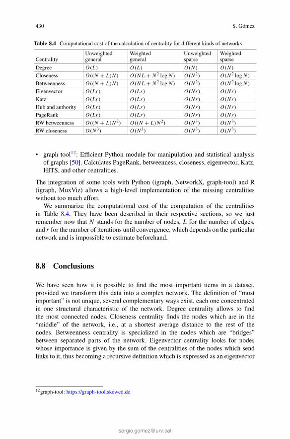
Table 8.1 Most central nodes of undirected network in Figs. 8.1 and 8.2
Centrality Most central Second most central Third most central
Degree 28 19, 24 6, 7, 10, 11, 16, 18, 20, 22
Closeness 18 24 16
Eigenvector 19 20, 22 21, 23
Katz 28 19 20, 22
Betweenness 28 24 18
PageRank 28 24 36, 39
Random-walk betweenness 28 18 24
Random-walk closeness 18 16 24
Table 8.2 Most central nodes of directed network in Figs. 8.3 and 8.4
Centrality Most central Second most central Third most central
Input degree 8, 14 25, 27 23
Output degree 13 1, 12 23, 27
Input closeness 14 22 20
Output closeness 13 19 16
Eigenvector 23 27 25
Katz 27 25 28, 29, 30, 31
Hub 13 12 1
Authority 14 8 7
Betweenness 20 23 8
PageRank 31 30 27
8.6 Examples
We have designed a couple of small networks, one undirected and the other directed,to grasp the differences between the most central nodes according to each of thedefinitions of centrality we have elaborated above. Figures 8.1 and 8.2 show themfor the undirected network, while Figs. 8.3 and 8.4 for the directed network. Inaddition, Tables 8.1 and 8.2 enumerate the most, second most, and third most centralnodes for the undirected and directed networks, respectively. These networks havebeen designed in such a way that each centrality measure leads to different mostcentral nodes, with few coincidences, to emphasize the topological features whichdistinguish them.
Fig. 8.1 Six different types of centralities for an undirected network. Nodes with highest centralityin dark red (and white node label), second largest centrality in red, third largest centrality in lightred, and rest of nodes in blue. Sizes proportional to centrality with an offset. (a) Degree centrality.(b) Closeness centrality. (c) Eigenvector centrality. (d) Katz centrality. (e) Betweenness centrality.(f) PageRank centrality
8 Centrality in Networks: Finding the Most Important Nodes 421
l
ll
l
ll
ll
ll
l
l
ll
l
l
l
l
l
ll
l
l
l
l
l
ll
l
l
l
l
l
l
1
2
34
5
6
78
9
10
1112
13
14
1516
17
18
19
2021
22
23
2425
26
27
2829
3031
32
33
34
35
36
37
38
39
40
41
42
43
44
(a)
ll
ll
l
l
l
l
ll
l
l
l
lll
l
l
l
l
l
l
ll
l
l
l
l
l
l
1
2
34
5
6
78
9
1011
12
13
14
1516
17
18
19
2021
22
23
2425
26
27
2829
3031
32
33
34
35
36
37
38
39
40
41
42
43
44
(b)
Fig. 8.2 Two random-walk based centralities for an undirected network. As in the previous figure,nodes with highest centrality in dark red (and white node label), second largest centrality in red,third largest centrality in light red, and rest of nodes in blue. Sizes proportional to centrality withan offset. (a) Random-walk betweenness centrality. (b) Random-walk closeness centrality
Looking at Figs. 8.1, 8.2, 8.3, and 8.4 we observe several patterns that deservea few words. First, the symmetries present in the networks are responsible for theexistence of several distinct nodes with exactly the same centralities. For example,in the undirected unweighted network in Figs. 8.1 and 8.2, nodes 20 and 22 havealways the same centrality, no matter the definition we choose, and the samehappens for many other tuples of nodes: (12, 15), (21, 23), (25, 26), (36, 39),(37, 38, 40, 41), (42, 43, 44), etc.; real networks are usually not so symmetric. Inthe directed network there are less symmetries: (4, 5, 6), (10, 11), and (17, 18).With respect to the relationship among the different centrality measures, the mostremarkable similarity appears between shortest-path betweenness centrality andrandom-walk betweenness centrality, which is not surprising at all, but there are alsoimportant differences. For example, node 27 has zero betweenness in the undirectednetwork since there is no shortest path crossing it, but it is among the ten nodes withhighest random-walk betweenness since it lays in a region which communicateswell-separated parts of the network. Another important feature in both networks isthat nodes with high degree frequently appear as top ranked for many centralities,showing the relevance of degree in the analysis of complex networks.
Fig. 8.3 Input and output degree, input and output closeness, eigenvector, and Katz centralities fora directed network. Nodes with highest centrality in dark red (and white node label), second largestcentrality in red, third largest centrality in light red, and rest of nodes in blue. Sizes proportional tocentrality with an offset. (a) Input degree centrality. (b) Output degree centrality. (c) Input closenesscentrality. (d) Output closeness centrality. (e) Eigenvector centrality. (f) Katz centrality
8 Centrality in Networks: Finding the Most Important Nodes 423
l
ll
l
l
ll
l
l
l
l
l
l
l
l
l
l
l
l
l
l
l
l
l
l
1
2
34
5
6
7
8
9
10
1112
13
14
15
16
17
18
19
20
21
22
23
24
25
26
27
28
29
30
31
(a)
l
l
ll
l
ll
l
l
l
l
l
l
l
l
l
l
l
l
l
1
2
34
5
6
7
8
9
10
1112
13
14
15
16
17
18
19
20
21
22
23
24
25
26
27
28
29
30
31
(b)
l
l
ll
l
l
l
l
l
l
l
l
l
l
l
l
l
l
l
l
l
l
l
l
1
2
34
5
6
7
8
9
10
1112
13
14
15
16
17
18
19
20
21
22
23
24
25
26
27
28
29
30
31
(c)
l
l
ll
l
l
l
l
l
l l
l
l
l
l
l
l
l
l
l
l
1
2
34
5
6
7
8
9
10
1112
13
14
15
16
17
18
19
20
21
22
23
24
25
26
27
28
29
30
31
(d)
Fig. 8.4 Hub, authority, betweenness, and PageRank centralities for a directed network. Nodeswith highest centrality in dark red (and white node label), second largest centrality in red, thirdlargest centrality in light red, and rest of nodes in blue. Sizes proportional to centrality withan offset. (a) Hub centrality. (b) Authority centrality. (c) Betweenness centrality. (d) PageRankcentrality
Although not directly related to the main topic of the book, we are going toanalyse now a real network which is easy to recognize for a large audience, andwhose results help in the understanding of the different definitions of centrality innetworks. This is the Network of Thrones2 [11], a network compiled from the third
2Network of Thrones: https://www.macalester.edu/~abeverid/thrones.html.
volume “A Storm of Swords” of the book series “A Song of Ice and Fire”, writtenby the novelist and screenwriter George R. R. Martin, and widely popularized bythe HBO TV series “Game of Thrones”, created by David Benioff and D. B. Weiss.The network contains the 107 characters of “A Storm of Swords” connected with352 weighted edges. Two characters (nodes) are linked when their names are foundin the book separated by at most 15 words, meaning they have interacted in someway. The weight counts the number of this kind of interactions.
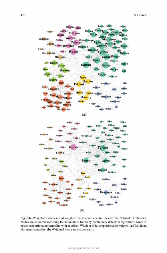
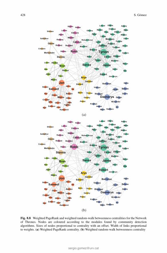
Since the Network of Thrones is weighted, we have opted here to use theweighted versions of several centrality measures, namely strength, closeness,betweenness, eigenvector, Katz, PageRank, random-walk betweenness, andrandom-walk closeness. For the weighted closeness and betweenness, we havereplaced the original weights wij by distances defined as dij = 1/wij , to takeinto account that the larger the weight, the smaller the distance (or dissimilarity)between the nodes. In Table 8.3 we show the 12 most central nodes for the degreecentrality and the eight weighted centralities mentioned above. Unlike the previoussynthetic networks, several characters are always among the most central nodes,with Tyrion Lannister on top of them, followed by Sansa Stark, Jaime Lannister, andRobb Stark, and to lower extend Jon Snow, Tywin Lannister and Cersei Lannister.
Figures 8.5, 8.6, 8.7, and 8.8 show the centralities of the Network of Thronesas proportional to the size of the nodes (and of the font of the names). The coloursof the nodes correspond to the seven modules found using two different communitydetection approaches [21, 28], which produce exactly the same partition: modularityoptimization [47] (using a combination of extremal optimization [26], tabu search[3], and fast algorithm [45]) and Infomap [53]. These communities are highlycorrelated with the different locations where the action takes place. A discussionin terms of overlapping communities for this network can be found in Chap. 9.
8 Centrality in Networks: Finding the Most Important Nodes 425
l
l
l
l
l
l
l
ll
l
l
lll
l
l
l
l
l
l
l
l
l
l
l
l
ll
l
l
l
l
l
l
l
l
ll
l
l
l
l
l
l
l
l
l
l
l
l
l
l
l
l
l
ll
l
l
ll
l
l
l
l
l
l
l
l
l
l
l
l
l
ll
l
l
l
l
l
l
l
ll
l
l Aegon
Aemon
Aerys
Alliser
Amory
Anguy
Arya
Balon
Barristan
Belwas
Beric
Bowen
Bran
Brienne
BronnBryndenCatelyn
Cersei
Chataya
Craster
Cressen
Daario
Daenerys
Dalla
Davos
Doran
Drogo
Eddard
Eddison
Edmure
Elia
Ellaria
Gendry
Gilly
Gregor
Grenn
Hodor
Hoster
Illyrio
Ilyn
Irri
Jaime
Janos
Jeyne
Joffrey
Jojen
Jon
Jon Arryn
Jorah
Karl
Kevan
Kraznys
Lancel
Loras
Lothar
Luwin
Lysa
Mace
Mance
Margaery
Marillion
Meera
Melisandre
Meryn
Missandei
Myrcella
Nan
OberynOlenna
Orell
Petyr
PodrickPycelle
Qhorin
Qyburn
Rakharo
Ramsay
Rattleshirt
Renly
Rhaegar
Rickard
Rickon
Robb
Robert
Robert Arryn
Roose
Roslin
Salladhor
Samwell
Sandor
Sansa
ShaeShireen
Stannis
Styr
Theon
Thoros
Tommen
Tyrion
Tywin
Val
Varys
Viserys
WalderWalton
Worm
Ygritte
(a)
l
l
l
l
l
l
l
l
ll
l
lll
l
l
l
l
l
ll
l
l
l
l
l
l
ll
l
l
l
l
l
l
l
l
ll
l
l
l
l
l
l
l
l
l
l
l
l
l
l
l
l
l
l
ll
l
l
ll
l
l
l
l
l
l
l
l
ll
l
l
l
l
l
ll
l
l
l
l
l
l
l
ll
ll Aegon
Aemon
Aerys
Alliser
Amory
Anguy
Arya
Balon
Barristan
Belwas
Beric
Bowen
Bran
Brienne
BronnBrynden
Catelyn
Cersei
Chataya
Craster
Cressen
Daario
Daenerys
Dalla
Davos
Doran
Drogo
Eddard
Eddison
Edmure
Elia
Ellaria
Gendry
Gilly
Gregor
Grenn
Hodor
Hoster
Illyrio
Ilyn
Irri
Jaime
Janos
Jeyne
Joffrey
Jojen
Jon
Jon Arryn
Jorah
Karl
Kevan
Kraznys
Lancel
Loras
Lothar
Luwin
Lysa
Mace
Mance
Margaery
Marillion
Meera
Melisandre
Meryn
Missandei
Myrcella
Nan
OberynOlenna
Orell
Petyr
PodrickPycelle
Qhorin
Qyburn
Rakharo
Ramsay
Rattleshirt
Renly
Rhaegar
Rickard
Rickon
Robb
Robert
Robert Arryn
Roose
Roslin
Salladhor
Samwell
Sandor
Sansa
ShaeShireen
Stannis
Styr
Theon
Thoros
Tommen
Tyrion
Tywin
Val
Varys
Viserys
WalderWalton
Worm
Ygritte
(b)
Fig. 8.5 Degree and strength centralities for the Network of Thrones. Nodes are colouredaccording to the modules found by community detection algorithms. Sizes of nodes proportional tocentrality with an offset. Width of links proportional to weights. (a) Degree centrality. (b) Strengthcentrality
Fig. 8.6 Weighted closeness and weighted betweenness centralities for the Network of Thrones.Nodes are coloured according to the modules found by community detection algorithms. Sizes ofnodes proportional to centrality with an offset. Width of links proportional to weights. (a) Weightedcloseness centrality. (b) Weighted betweenness centrality
8 Centrality in Networks: Finding the Most Important Nodes 427
l
l
l
l
l
l
l
l
ll
l
ll
l
l
l
ll
l
l
l
l
l
l
l
l
l
ll
l
l
l
l
l
l
l
l
l
l
l
l
l
l
l
l
l
l
l
l
l
l
l
l
l
l
l
l
l
l
ll
l
l
ll
l
l
l
l
l
l
l
l
ll
l
l
l
l
l
l
ll
l
l
l
l
l
l
l
l
ll
l
l Aegon
Aemon
Aerys
Alliser
Amory
Anguy
Arya
Balon
Barristan
Belwas
Beric
Bowen
Bran
BrienneBronnBrynden
Catelyn
Cersei
Chataya
Craster
Cressen
Daario
Daenerys
Dalla
Davos
Doran
Drogo
Eddard
Eddison
Edmure
Elia
Ellaria
Gendry
Gilly
Gregor
Grenn
Hodor
Hoster
Illyrio
Ilyn
Irri
Jaime
Janos
Jeyne
Joffrey
Jojen
Jon
Jon Arryn
Jorah
Karl
Kevan
Kraznys
Lancel
Loras
Lothar
Luwin
Lysa
Mace
Mance
Margaery
Marillion
Meera
Melisandre
Meryn
Missandei
Myrcella
Nan
OberynOlenna
Orell
Petyr
PodrickPycelle
Qhorin
Qyburn
Rakharo
Ramsay
Rattleshirt
Renly
Rhaegar
Rickard
Rickon
Robb
Robert
Robert Arryn
Roose
Roslin
Salladhor
Samwell
Sandor
Sansa
ShaeShireen
Stannis
Styr
Theon
Thoros
Tommen
Tyrion
Tywin
Val
Varys
Viserys
WalderWalton
Worm
Ygritte
(a)
l
l
l
l
l
l
l
l
ll
l
ll
l
l
l
ll
l
l
l
l
l
l
l
l
l
ll
l
l
l
l
l
l
l
l
ll
l
l
l
l
l
l
l
l
l
l
l
l
l
l
l
l
l
l
l
ll
l
l
ll
l
l
l
l
l
l
l
l
ll
l
l
l
l
l
ll
l
l
l
l
l
l
l
l
ll
ll Aegon
Aemon
Aerys
Alliser
Amory
Anguy
Arya
Balon
Barristan
Belwas
Beric
Bowen
Bran
BrienneBronnBrynden
Catelyn
Cersei
Chataya
Craster
Cressen
Daario
Daenerys
Dalla
Davos
Doran
Drogo
Eddard
Eddison
Edmure
Elia
Ellaria
Gendry
Gilly
Gregor
Grenn
Hodor
Hoster
Illyrio
Ilyn
Irri
Jaime
Janos
Jeyne
Joffrey
Jojen
Jon
Jon Arryn
Jorah
Karl
Kevan
Kraznys
Lancel
Loras
Lothar
Luwin
Lysa
Mace
Mance
Margaery
Marillion
Meera
Melisandre
Meryn
Missandei
Myrcella
Nan
OberynOlenna
Orell
Petyr
PodrickPycelle
Qhorin
Qyburn
Rakharo
Ramsay
Rattleshirt
Renly
Rhaegar
Rickard
Rickon
Robb
Robert
Robert Arryn
Roose
Roslin
Salladhor
Samwell
Sandor
Sansa
ShaeShireen
Stannis
Styr
Theon
Thoros
Tommen
Tyrion
Tywin
Val
Varys
Viserys
WalderWalton
Worm
Ygritte
(b)
Fig. 8.7 Weighted eigenvector and weighted Katz centralities for the Network of Thrones. Nodesare coloured according to the modules found by community detection algorithms. Sizes of nodesproportional to centrality with an offset. Width of links proportional to weights. (a) Weightedeigenvector centrality. (b) Weighted Katz centrality
Fig. 8.8 Weighted PageRank and weighted random-walk betweenness centralities for the Networkof Thrones. Nodes are coloured according to the modules found by community detectionalgorithms. Sizes of nodes proportional to centrality with an offset. Width of links proportionalto weights. (a) Weighted PageRank centrality. (b) Weighted random-walk betweenness centrality
8 Centrality in Networks: Finding the Most Important Nodes 429
8.7 Software and Cost
Here comes a list of software tools which can be used to calculate centralities incomplex networks:
• Pajek3: Analysis and visualization tool for Windows (can be run under Linuxand MacOS using Wine) [7]. Allows the calculation of several centralities:degree, strength, closeness, betweenness, hubs and authorities (HITS), and a fewadditional ones not described above.
• Gephi4: Visualization and exploration software [6]. Calculates degree, strength,eigenvector, HITS, and PageRank centralities.
• Radatools5: Set of programs for the analysis of complex networks, with mainattention to community detection and the finding of structural properties [33].Calculates degree, strength, betweenness (weighted and unweighted, directedand undirected, for nodes and edges), and other centralities.
• Cytoscape6: Originally designed for biological research, now it is a generalplatform for complex network analysis and visualization [56]. It does not directlycalculate centralities, but there are plug-ins which can be used to find some ofthem.
• igraph7: Collection of network analysis tools with the emphasis on efficiency,portability, and ease of use [20]. Calculates degree, strength, betweenness,closeness, eigenvector, HITS, and PageRank centralities.
• NetworkX8: Python software package for the creation, manipulation, and studyof the structure, dynamics, and functions of complex networks [55]. Calculatesdegree, strength, closeness, betweenness, eigenvector, HITS, Katz and PageRankcentralities, and a few additional ones.
• SNAP9: General purpose, high performance system for analysis, and manipula-tion of large networks [42]. Calculates degree, strength, closeness, betweenness,eigenvector, and HITS centralities.
• Visone10: Tool for the analysis and visualization of social networks [18]. Calcu-lates degree, strength, closeness, betweenness, eigenvector, HITS and PageRankcentralities, and a few additional ones.
• MuxViz11: Framework for the multilayer analysis and visualization of networks[22]. Calculates the generalizations of centralities to multilayer networks (versa-tilities), including degree, eigenvector, Katz, HITS, and PageRank centralities.
• graph-tool12: Efficient Python module for manipulation and statistical analysisof graphs [50]. Calculates PageRank, betweenness, closeness, eigenvector, Katz,HITS, and other centralities.
The integration of some tools with Python (igraph, NetworkX, graph-tool) and R(igraph, MuxViz) allows a high-level implementation of the missing centralitieswithout too much effort.
We summarize the computational cost of the computation of the centralitiesin Table 8.4. They have been described in their respective sections, so we justremember now that N stands for the number of nodes, L for the number of edges,and r for the number of iterations until convergence, which depends on the particularnetwork and is impossible to estimate beforehand.
8.8 Conclusions
We have seen how it is possible to find the most important items in a dataset,provided we transform this data into a complex network. The definition of “mostimportant” is not unique, several complementary ways exist, each one concentratedin one structural characteristic of the network. Degree centrality allows to findthe most connected nodes. Closeness centrality finds the nodes which are in the“middle” of the network, i.e., at a shortest average distance to the rest of thenodes. Betweenness centrality is specialized in the nodes which are “bridges”between separated parts of the network. Eigenvector centrality looks for nodeswhose importance is given by the sum of the centralities of the nodes which sendlinks to it, thus becoming a recursive definition which is expressed as an eigenvector
8 Centrality in Networks: Finding the Most Important Nodes 431
and eigenvalue problem. Katz centrality represents a balance between closeness andeigenvector centralities. Finally, the dynamics of random walkers in the network isthe basis for several centralities, standing out PageRank, the well-known measureoriginally used to rank web pages by the Google search engine. We have alsoconsidered how centralities must be adapted for the different kinds of network,e.g., by taking into account the directionality of the links, their weights, or themultilayer structure. In summary, centrality integrates a large set of definitions andtools to analyse the relevance of the nodes in networks, being able to identify themost important ones, which may constitute the first step in many marketing andbusiness applications, where targeted actions increase their success rate and reducethe overall cost.
Acknowledgements S.G. acknowledges funding from the Spanish Ministerio de Economía yCompetitividad (grant number FIS2015-71582-C2-1).
References
1. Ahnert, S., Garlaschelli, D., Fink, T., Caldarelli, G.: Ensemble approach to the analysis ofweighted networks. Physical Review E 76(1), 016,101 (2007)
2. Anthonisse, J.M.: The rush in a directed graph. Stichting Mathematisch Centrum. Mathematis-che Besliskunde (BN 9/71), 1–10 (1971)
3. Arenas, A., Fernandez, A., Gomez, S.: Analysis of the structure of complex networks atdifferent resolution levels. New Journal of Physics 10(5), 053,039 (2008)
4. Barabási, A.L., Albert, R.: Emergence of scaling in random networks. Science 286(5439),509–512 (1999)
5. Barrat, A., Barthelemy, M., Pastor-Satorras, R., Vespignani, A.: The architecture of complexweighted networks. Proceedings of the National Academy of Sciences USA 101(11), 3747–3752 (2004)
6. Bastian, M., Heymann, S., Jacomy, M., et al.: Gephi: an open source software for exploringand manipulating networks. ICWSM 8, 361–362 (2009)
7. Batagelj, V., Mrvar, A.: Pajek – program for large network analysis. Connections 21(2), 47–57(1998)
8. Battiston, F., Nicosia, V., Latora, V.: Structural measures for multiplex networks. PhysicalReview E 89(3), 032,804 (2014)
9. Bavelas, A.: Communication patterns in task-oriented groups. The Journal of the AcousticalSociety of America 22(6), 725–730 (1950)
10. Beauchamp, M.A.: An improved index of centrality. Behavioral Science 10(2), 161–163 (1965)11. Beveridge, A., Shan, J.: Network of thrones. Math Horizons 23(4), 18–22 (2016)12. Boccaletti, S., Bianconi, G., Criado, R., Del Genio, C.I., Gómez-Gardenes, J., Romance, M.,
Sendina-Nadal, I., Wang, Z., Zanin, M.: The structure and dynamics of multilayer networks.Physics Reports 544(1), 1–122 (2014)
13. Bonacich, P.: Factoring and weighting approaches to status scores and clique identification.Journal of Mathematical Sociology 2(1), 113–120 (1972)
18. Brandes, U., Wagner, D.: Analysis and visualization of social networks. Graph drawingsoftware pp. 321–340 (2004)
19. Brin, S., Page, L.: The anatomy of a large-scale hypertextual web search engine. ComputerNetworks and ISDN Systems 30(1), 107–117 (1998)
20. Csardi, G., Nepusz, T.: The igraph software package for complex network research. InterJour-nal, Complex Systems 1695(5), 1–9 (2006)
21. Danon, L., Diaz-Guilera, A., Duch, J., Arenas, A.: Comparing community structure identifica-tion. Journal of Statistical Mechanics: Theory and Experiment 2005(09), P09,008 (2005)
22. De Domenico, M., Porter, M.A., Arenas, A.: Muxviz: a tool for multilayer analysis andvisualization of networks. Journal of Complex Networks 3(2), 159 (2015).
23. De Domenico, M., Solé-Ribalta, A., Cozzo, E., Kivelä, M., Moreno, Y., Porter, M.A., Gómez,S., Arenas, A.: Mathematical formulation of multilayer networks. Physical Review X 3(4),041,022 (2013)
24. De Domenico, M., Solé-Ribalta, A., Omodei, E., Gómez, S., Arenas, A.: Ranking in intercon-nected multilayer networks reveals versatile nodes. Nature Communications 6 (2015)
25. Dekker, A.: Conceptual distance in social network analysis. Journal of Social Structure (JOSS)6 (2005)
26. Duch, J., Arenas, A.: Community detection in complex networks using extremal optimization.Physical review E 72(2), 027,104 (2005)
27. Floyd, R.W.: Algorithm 97: shortest path. Communications of the ACM 5(6), 345 (1962)28. Fortunato, S.: Community detection in graphs. Physics reports 486(3), 75–174 (2010)29. Freeman, L.C.: A set of measures of centrality based on betweenness. Sociometry pp. 35–41
(1977)30. Freeman, L.C.: Centrality in social networks conceptual clarification. Social Networks 1(3),
215–239 (1979)31. Frobenius, G.: Über matrizen aus nicht negativen elementen. Sitzungsber. Königl. Preuss.
Akad. Wiss. pp. 456–477 (1912)32. Garrison, W.L.: Connectivity of the interstate highway system. Papers and Proceedings of the
Regional Science Association 6, 121–137 (1960)33. Gómez, S., Fernández, A.: Radatools software, communities detection in complex networks
and other tools (2011)34. Guimerà, R., Diaz-Guilera, A., Vega-Redondo, F., Cabrales, A., Arenas, A.: Optimal network
topologies for local search with congestion. Physical Review Letters 89(24), 248,701 (2002)35. Halu, A., Mondragón, R.J., Panzarasa, P., Bianconi, G.: Multiplex pagerank. PLOS ONE 8(10),
e78,293 (2013)36. Jacob, R., Koschützki, D., Lehmann, K., Peeters, L., Tenfelde-Podehl, D.: Algorithms for
centrality indices. Network Analysis pp. 62–82 (2005)37. Katz, L.: A new status index derived from sociometric analysis. Psychometrika 18(1), 39–43
(1953)38. Kivelä, M., Arenas, A., Barthelemy, M., Gleeson, J.P., Moreno, Y., Porter, M.A.: Multilayer
networks. Journal of Complex Networks 2(3), 203–271 (2014)39. Kleinberg, J.M.: Authoritative sources in a hyperlinked environment. Journal of the ACM
(JACM) 46(5), 604–632 (1999)40. Koschützki, D., Lehmann, K., Peeters, L., Richter, S., Tenfelde-Podehl, D., Zlotowski, O.:
Centrality indices. Network Analysis pp. 16–61 (2005)41. Koschützki, D., Lehmann, K., Tenfelde-Podehl, D., Zlotowski, O.: Advanced centrality
concepts. Network Analysis pp. 83–111 (2005)42. Leskovec, J., Sosic, R.: Snap: Stanford network analysis platform (2013)43. Lovász, L.: Random walks on graphs: A survey. Combinatorics, Paul Erdos is Eighty 2(1),
8 Centrality in Networks: Finding the Most Important Nodes 433
44. Newman, M.: Networks: An Introduction. Oxford University Press, Inc., New York, NY, USA(2010)
45. Newman, M.E.: Fast algorithm for detecting community structure in networks. Physical reviewE 69(6), 066,133 (2004)
46. Newman, M.E.: A measure of betweenness centrality based on random walks. Social Networks27(1), 39–54 (2005)
47. Newman, M.E., Girvan, M.: Finding and evaluating community structure in networks. Physicalreview E 69(2), 026,113 (2004)
48. Nieminen, J.: On the centrality in a directed graph. Social Science Research 2, 371–378 (1973)49. Noh, J.D., Rieger, H.: Random walks on complex networks. Physical Review Letters. 92(11),
118,701 (2004)50. Peixoto, T.P.: The graph-tool python library. figshare (2014)51. Perron, O.: Zur theorie der matrices. Mathematische Annalen 64(2), 248–263 (1907)52. Pitts, F.R.: A graph theoretic approach to historical geography. The Professional Geographer
17, 15–20 (1965)53. Rosvall, M., Bergstrom, C.T.: Maps of random walks on complex networks reveal community
structure. Proceedings of the National Academy of Sciences 105(4), 1118–1123 (2008)54. Sabidussi, G.: The centrality index of a graph. Psychometrika 31, 581–603 (1966)55. Schult, D.A., Swart, P.: Exploring network structure, dynamics, and function using networkx.
In: Proceedings of the 7th Python in Science Conferences (SciPy 2008), vol. 2008, pp. 11–16(2008)
56. Shannon, P., Markiel, A., Ozier, O., Baliga, N.S., Wang, J.T., Ramage, D., Amin, N.,Schwikowski, B., Ideker, T.: Cytoscape: a software environment for integrated models ofbiomolecular interaction networks. Genome research 13(11), 2498–2504 (2003)
57. Shaw, M.E.: Group structure and the behavior of individuals in small groups. Journal ofPsychology 38, 139–149 (1954)
58. Solá, L., Romance, M., Criado, R., Flores, J., del Amo, A.G., Boccaletti, S.: Eigenvectorcentrality of nodes in multiplex networks. Chaos 3, 033,131 (2013)
59. Solé-Ribalta, A., De Domenico, M., Gómez, S., Arenas, A.: Random walk centrality ininterconnected multilayer networks. Physica D: Nonlinear Phenomena 323, 73–79 (2016)
60. Solé-Ribalta, A., Gómez, S., Arenas, A.: A model to identify urban traffic congestion hotspotsin complex networks. Royal Society Open Science 3(10), 160,098 (2016)
61. Yang, S.J.: Exploring complex networks by walking on them. Physical Review E 71(1),016,107 (2005)
62. Zhang, Z., Julaiti, A., Hou, B., Zhang, H., Chen, G.: Mean first-passage time for random walkson undirected networks. The European Physical Journal B-Condensed Matter and ComplexSystems 84(4), 691–697 (2011)