Chapter 8 Cohort studies - · PDF filestudy (e.g., cross-sectional or case–control...

165

A cohort study is an observational study in which a study population (acohort) is selected and information is obtained to determine which sub-jects either have a particular characteristic (e.g., blood group A) that is sus-pected of being related to the development of the disease under investiga-tion, or have been exposed to a possible etiological agent (e.g., cigarettesmoking). The entire study population is then followed up in time, andthe incidence of the disease in the exposed individuals is compared withthe incidence in those not exposed.

Thus cohort studies resemble intervention studies in that people areselected on the basis of their exposure status and then followed up in time,but differ from them in that the allocation to the study groups is notunder the direct control of the investigators.

In , a group of 22 707 Chinese male government employ-ees (the ‘cohort’) was assembled and their HBsAg status (the ‘exposure’)determined at the start of the study. They were then followed up forseveral years to measure (and compare) the incidence of hepatocellularcarcinoma (the ‘outcome’) in subjects who were HBsAg-positive or HBsAg-negative at the time of entry into the study.

As in any other study design, it is essential that a clear hypothesis isformulated before the start of a cohort study. This should include a cleardefinition of the exposure(s) and outcome(s) of interest. Since cohort stud-ies in cancer epidemiology often involve follow-up of a large number ofpeople for a long period of time, they tend to be very expensive and time-consuming. Consequently, such studies are generally carried out after ahypothesis has been explored in other (cheaper and quicker) types of

Chapter 8

Example 8.1. A cohort study of 22 707 Chinese men in Taiwan was setup to investigate the association between the hepatitis B surface antigen(HBsAg) and the development of primary hepatocellular carcinoma. Thestudy was conducted among male government employees who were enrolledthrough routine health care services. All participants completed a healthquestionnaire and provided a blood sample at the time of their entry into thestudy. Participants were then followed up for an average of 3.3 years(Beasley et al., 1981).

Text book eng. Chap.8 final 27/05/02 9:45 Page 165 (Black/Process Black film)

Example 8.1

8.1 Definition of the objectives

Cohort studies

Example 8.1. A cohort study of 22 707 Chinese men in Taiwan was setup to investigate the association between the hepatitis B surface antigen(HBsAg) and the development of primary hepatocellular carcinoma. Thestudy was conducted among male government employees who were enrolledthrough routine health care services. All participants completed a healthquestionnaire and provided a blood sample at the time of their entry into thestudy. Participants were then followed up for an average of 3.3 years(Beasley et al., 1981).

Text book eng. Chap.8 final 27/05/02 9:45 Page 165 (Black/Process Black film)TextText book book book eng. eng. eng. Chap.8 Chap.8 Chap.8 final final final 27/05/02 27/05/02 27/05/02 9:45 9:45 9:45 Page Page Page 165 165 165 (PANTONE (PANTONE (Black/Process 313 313 (Black/Process CV CV (Black/Process film) film) Black

study (e.g., cross-sectional or case–control studies). For instance, thecohort study in Taiwan ( ) was set up only after a series ofcase–control studies of hepatocellular carcinoma had been carried out inthe early and mid-1970s (IARC, 1994b).

The choice of a particular group to serve as the study population for anygiven cohort study depends on the specific hypothesis under investigationand on practical constraints. The cohort chosen may be a general popula-tion group, such as the residents of a community, or a more narrowlydefined population that can be readily identified and followed up, such asmembers of professional or social organizations (e.g., members of healthinsurance schemes, registered doctors and nurses). Alternatively, thecohort may be selected because of high exposure to a suspected etiologicalfactor, such as a source of ionizing radiation, a particular type of treatment(e.g., chemotherapy, radiotherapy) or an occupational hazard.

A general population cohort may be drawn from a geographically welldefined area (as in ), which is initially surveyed to establishbaseline exposure status with respect to a number of factors and thenexamined periodically to ascertain disease outcomes.

One of the great advantages of this type of cohort study is that it allowsa large number of common exposures to be considered in relation to alarge number of outcomes. The Framingham Study is a classical exampleof this. Approximately 5000 residents of the town of Framingham, inMassachusetts (USA), have been followed up since 1948 (Dawber et al.,1951). There were several reasons for selecting this location for the study,mainly determined by logistic and other practical considerations to ensurethat it would be feasible to identify and follow participants for manyyears. At the time the study was set up, Framingham was a relatively sta-ble community including both industrial and rural areas, with a numberof occupations and industries represented. The town was small enough toallow residents to come to one central examining facility and there wasonly one major hospital. Follow-up of this cohort has permitted assess-ment of the effects of a wide variety of factors (e.g., blood pressure, serum

Chapter 8

166

Example 8.2. A cohort of 10 287 individuals resident in the Ernakulamdistrict of Kerala (India) were followed up for a 10-year period to assess theeffect of tobacco chewing and smoking habits on overall mortality.Participants were initially identified through a baseline survey in which anumber of villages in the district were randomly selected. All residents in theselected villages aged 15 years and over were interviewed about their tobac-co habits in a house-to-house survey and entered into the cohort. Refusalswere negligible (Gupta et al., 1984).


Example 8.1

8.2 Choice of the study population8.2.1 Source of the study population

Example 8.2

Example 8.2. A cohort of 10 287 individuals resident in the Ernakulamdistrict of Kerala (India) were followed up for a 10-year period to assess theeffect of tobacco chewing and smoking habits on overall mortality.Participants were initially identified through a baseline survey in which anumber of villages in the district were randomly selected. All residents in theselected villages aged 15 years and over were interviewed about their tobac-co habits in a house-to-house survey and entered into the cohort. Refusalswere negligible (Gupta et al., 1984).


cholesterol, alcohol intake, physical exercise, smoking) on the risk ofnumerous diseases, ranging from cardiovascular diseases and cancer togout, gallbladder disease and eye conditions.

Alternatively, it can be preferable for logistic reasons to draw a generalpopulation cohort from a well defined socio-professional group of indi-viduals. For instance, the Taiwan study described in was con-ducted among civil servants not because they were thought to have ahigher exposure to hepatitis B virus than the rest of the population, butbecause this group of people was easier to identify and to follow than anyother potential study population.

Similarly, when Richard Doll and Bradford Hill set up a cohort study inEngland and Wales to assess the health effects of smoking, the choice ofthe British physicians as the study population ( ) was deter-mined mainly by logistic considerations. Physicians were registered withthe British Medical Association and were therefore easy to identify and fol-low up. Besides, they were more likely to cooperate and the cause of deathto be properly investigated.

If the exposure is rare, a study of the general population will have littleability to detect an effect (i.e., the study would have insufficient statisti-cal power (see Chapter 15)), since very few people would have beenexposed to the factor of interest. This problem can be overcome by delib-erately selecting a highly exposed group of people as the study population.For example, exposure to dyestuffs is rare in the general population.However, by choosing a group of workers with high exposure, the fullrange of effects of the exposure on their health can be studied, includingoutcomes that are rare in the general population but not in those heavi-ly exposed. The general public health impact of the exposure may besmall, but such studies can give insight into common biological mecha-nisms in disease.

Cohort studies

167

Example 8.3. A postal questionnaire was sent in 1951 to all men andwomen whose names were at that time on the British Medical Register andwho were believed to be resident in the United Kingdom. In addition toname, address and age, they were asked a few simple questions about theirsmoking habits. A total of 34 439 male and 6194 female doctors providedsufficiently complete replies. These doctors have been followed up since then(Doll & Hill, 1954; Doll & Peto, 1976; Doll et al., 1980, 1994a,b).

Example 8.4. The Life Span Study is an on-going cohort study which wasset up to investigate the long-term health effects of exposure to high levels ofionizing radiation among survivors of the atomic bomb explosions in Japan.It comprises a sample of 120 128 subjects who were resident in Hiroshimaand Nagasaki in 1950, when the follow-up began (Shimizu et al., 1990).


Example 8.1

Example 8.3

Example 8.3. A postal questionnaire was sent in 1951 to all men andwomen whose names were at that time on the British Medical Register andwho were believed to be resident in the United Kingdom. In addition toname, address and age, they were asked a few simple questions about theirsmoking habits. A total of 34 439 male and 6194 female doctors providedsufficiently complete replies. These doctors have been followed up since then(Doll & Hill, 1954; Doll & Peto, 1976; Doll et al., 1980, 1994a,b).

Example 8.4. The Life Span Study is an on-going cohort study which wasset up to investigate the long-term health effects of exposure to high levels ofionizing radiation among survivors of the atomic bomb explosions in Japan.It comprises a sample of 120 128 subjects who were resident in Hiroshimaand Nagasaki in 1950, when the follow-up began (Shimizu et al., 1990).


The follow-up of the survivors of the atomic bomb explosions in Japan( ) has not only clarified many of the long-term health effectsof acute exposure to high levels of ionizing radiation, but has also con-tributed to our understanding of the effects of chronic exposure to low-level radiation.

Once the source of exposed subjects has been determined, the next stepis to select an appropriate comparison group of unexposed individuals.This selection is the most critical aspect in the design of a cohort study.The unexposed group should be as similar as possible to the exposed groupwith respect to the distribution of all factors that may be related to theoutcome(s) of interest except the exposure under investigation. In otherwords, if there were really no association between the exposure and thedisease, the disease incidence in the two groups being compared would beessentially the same. Two main types of comparison group may be used ina cohort study: internal and external.

General population cohorts tend to be heterogeneous with respect tomany exposures and, hence, their members can be classified into differentexposure categories. In such circumstances, an internal comparison groupcan be utilized. That is, the experience of those members of the cohortwho are either unexposed or exposed to low levels can be used as the com-parison group. For example, in the cohort study of British physicians( ), it was possible to categorize individuals in terms of theirsmoking habits and then compare the mortality from lung cancer (andother conditions) in smokers with mortality in non-smokers.

In , a portion of the cohort of US registered female nurseswas taken as the ‘unexposed group’ to examine the relationship betweenoral contraceptive use and risk of developing breast cancer.

In general population cohorts, it is possible to examine the effect ofmore than one exposure. Thus, the choice of the group of people in thecohort who will be regarded as ‘unexposed’ depends on the particularexposure under investigation. For instance, the Nurses’ Health Study hasalso allowed examination of the relationship between dietary total fat

Chapter 8

168

Example 8.5. The Nurses’ Health Study was established in 1976, when acohort of 121 700 US female registered nurses aged 30–55 years completeda questionnaire on medical conditions and lifestyle practices. A total of 1799newly diagnosed breast cancer cases occurred during the first 10 years of fol-low-up from mid-1976 to mid-1986. Analyses were then conducted to inves-tigate the relationship between oral contraceptive use and risk of breast can-cer. Women who reported in the initial questionnaire in 1976 and in subse-quent ones to have never taken oral contraceptives were considered as the‘unexposed’ group in this analysis (Romieu et al., 1989).


Example 8.4

8.2.2 Choice of the comparison group

Example 8.3

Example 8.5

Example 8.5. The Nurses’ Health Study was established in 1976, when acohort of 121 700 US female registered nurses aged 30–55 years completeda questionnaire on medical conditions and lifestyle practices. A total of 1799newly diagnosed breast cancer cases occurred during the first 10 years of fol-low-up from mid-1976 to mid-1986. Analyses were then conducted to inves-tigate the relationship between oral contraceptive use and risk of breast can-cer. Women who reported in the initial questionnaire in 1976 and in subse-quent ones to have never taken oral contraceptives were considered as the‘unexposed’ group in this analysis (Romieu et al., 1989).


intake and the risk of breast cancer. For this purpose, nurses were asked tocomplete a dietary questionnaire and the distribution of fat intake in thewhole cohort was examined and divided into five groups of equal size(‘quintiles’); women in the lowest quintile of fat intake were taken as the‘unexposed group’ (Willett et al., 1987).

In occupational cohorts, an internal comparison group might consist ofworkers within the same facility with other types of job not involvingexposure to the factor under investigation.

In , it was possible to identify a group of workers who couldbe regarded as unexposed to external radiation on the basis of personal doserecords.

When the cohort is essentially homogeneous in terms of exposure to thesuspected factor, a similar but unexposed cohort, or some other standard ofcomparison, is required to evaluate the experience of the exposed group. Forexample, in some occupational cohorts it is not possible to identify a sub-group of the cohort that can be considered as ‘unexposed’ for comparison.In this instance, an external comparison group must be used. A potential com-parison group is a cohort of similar workers in another occupation whichdoes not involve exposure to the factor of interest. For instance, many occu-pational exposures only occur among certain workforces and therefore itcan often be assumed that the level of exposure of other workforces is vir-tually zero. We can therefore choose people in employment from the samegeographical area, who are not exposed to the risk factor of interest, as acomparison group. It is important to ensure that the risk of disease in theseworkforces is not affected by their own occupational exposures.

Alternatively, the general population of the geographical area in whichthe exposed individuals reside may be taken as the external comparisongroup. In this case, the disease experience observed in the cohort is com-pared with the disease experience of the general population at the time thecohort is being followed. Comparison with rates in the general population

Cohort studies

169

Example 8.6. A cohort of all 14 282 workers employed at the Sellafieldplant of British Nuclear Fuels at any time between the opening of the site in1947 and 31 December 1975 was identified retrospectively from employ-ment records. Employees who worked in areas of the plant where they werelikely to be exposed to external radiation wore film badge dosimeters andthese personal dose records were kept by the industry. These workers wereconsidered in the present study as ‘radiation workers’, while those who neverwore film badges were taken as ‘non-radiation’ workers. It was initiallyplanned to follow up the workers from the time they joined the workforce upto the end of 1975, but the follow-up period was later extended to the endof 1988. The mortality experienced by the ‘radiation workers’ was then com-pared with that experienced by the ‘non-radiation workers’ (Smith &Douglas, 1986; Douglas et al., 1994).


Example 8.6

Example 8.6. A cohort of all 14 282 workers employed at the Sellafieldplant of British Nuclear Fuels at any time between the opening of the site in1947 and 31 December 1975 was identified retrospectively from employ-ment records. Employees who worked in areas of the plant where they werelikely to be exposed to external radiation wore film badge dosimeters andthese personal dose records were kept by the industry. These workers wereconsidered in the present study as ‘radiation workers’, while those who neverwore film badges were taken as ‘non-radiation’ workers. It was initiallyplanned to follow up the workers from the time they joined the workforce upto the end of 1975, but the follow-up period was later extended to the endof 1988. The mortality experienced by the ‘radiation workers’ was then com-pared with that experienced by the ‘non-radiation workers’ (Smith &Douglas, 1986; Douglas et al., 1994).


avoids the need to follow up a large number of unexposed individuals, butit has several disadvantages. First, it can be done only for outcomes forwhich such information exists for the general population. Second, itassumes that only a very small proportion of the general population isexposed to the risk factor of interest, otherwise the presence of the exposurein the comparison group will lead to a gross underestimation of its trueeffect. Third, even if the general population is chosen to be as similar as pos-sible to the exposed cohort in relation to basic demographic and geograph-ic characteristics, it may well differ with respect to other risk factors for thedisease, such as diet, smoking, etc. Since this information is not available onindividuals in a general population, any observed differences may in fact bedue to the effects of confounding that cannot be controlled.

The advantage of using another special group of people as the externalunexposed comparison group rather than making comparison with diseaserates of the general population is that the group can be selected to be moresimilar to the exposed cohort than the general population would be.Moreover, information on potential confounding factors can be obtainedfrom all exposed and unexposed individuals in the study and differencescontrolled for in the analysis.

In many cohort studies, it may be useful to have multiple comparisongroups, especially when we cannot be sure that any single group will be suf-ficiently similar to the exposed group in terms of the distribution of poten-tial confounding variables. In such circumstances, the study results may bemore convincing if a similar association were observed for a number of dif-ferent comparison groups. For instance, with some occupational cohortsboth an internal comparison group (people employed in the same factorybut having a different job) and the experience of the general population(national and local rates) may be used.

In , the all-cause mortality of the cohort of rubber workerswas compared with the mortality of another industrial cohort and with local(state) and national rates. Note that both the rubber and the steel workersexperienced lower age-specific death rates than either the state or thenational populations. This is because people who work tend to be healthierthan the general population, which includes those who are too ill or dis-abled to work (although for steel workers the difference may be due partlyto changes in mortality over time). This well known selection bias is calledthe ‘healthy worker effect’.

The healthy worker effect may conceal true increases in the risk of a dis-ease in relation to a particular exposure. It is known to vary with type of dis-ease, being smaller for cancer than for other major diseases, and it tends todisappear with time since recruitment into the workforce (see Section13.1.1). If rates in the occupational cohort remain lower than those from thegeneral population throughout the follow-up period, this is more likely tobe due to sociodemographic and lifestyle differences between the workforceand the general population than to the selection of healthy individuals atthe time of recruitment.

Chapter 8

170


Example 8.7


This health selection effect is not restricted to occupational cohorts. A sim-ilar phenomenon has been observed in many other types of cohort study. Inthe British doctors study described in , those who replied to theinitial questionnaire had a much lower mortality in the first years of follow-up than those who did not reply (Doll & Hill, 1954). Less health-consciouspeople, or those already suffering from health problems, might have felt lessmotivated to participate.

Measurement of the exposure(s) of interest is acrucial aspect in the design of a cohort study.Information should be obtained on age at first expo-sure, dates at which exposure started and stopped,dose and pattern of exposure (intermittent versusconstant), and changes over time (see Section 2.3).

Information on the exposure(s) of interest may beobtained from a number of sources, includingrecords collected independently of the study (e.g.,medical, employment or union records); informa-tion supplied by the study subjects themselves,through personal interviews or questionnaires; dataobtained by medical examination or other testing ofthe participants; biological specimens; or directmeasurements of the environment in which cohortmembers have lived or worked. The advantages and limitations of each ofthese sources were discussed in Chapter 2.

Cohort studies

171

Example 8.7. A cohort of workers in a major tyre-manufacturing plant inAkron, Ohio (USA) was set up to examine their overall and cause-specificmortality. A total of 6678 male rubber workers aged 40 to 84 at 1 January1964 were identified retrospectively from pension, payroll, death claims andother company files. These workers were followed from 1964 to 1972. Theage-specific mortality experienced by this cohort was then compared withthat experienced by three comparison groups–an industrial cohort of steelworkers, the population of the state where the plant is located (Ohio) and theUS national population (Table 8.1) (McMichael et al., 1974).

Age-specific mortality rate (per 100 000 pyrs)

Age-group Rubber worker cohort Steel worker cohort Ohio state USA(years)b (1964–72) (1953–61) (1972) (1968)

45–54 852 907 940 980

55–64 2317 2166 2365 2370

a Data from McMichael et al. (1974).

b Only data for these two age-groups were available for all the four populations.

Male age-specific mortality rates from

all causes in the rubber worker cohort

and in three other comparison groups:

steel workers, Ohio state population

and USA national population.a

Outline of (a) a prospective cohort

study and (b) a historical cohort study.

PAST PRESENT FUTURE

TIME

PAST PRESENT FUTURE

TIME

Study population

ExposedOutcome

No outcome

Outcome

No outcomeUnexposed

Study population

ExposedOutcome

No outcome

Outcome

No outcomeUnexposed

Outcome

No outcome

Outcome

No outcome

(a)

(b)


Example 8.3

8.3 Measurement of exposure

Example 8.7. A cohort of workers in a major tyre-manufacturing plant inAkron, Ohio (USA) was set up to examine their overall and cause-specificmortality. A total of 6678 male rubber workers aged 40 to 84 at 1 January1964 were identified retrospectively from pension, payroll, death claims andother company files. These workers were followed from 1964 to 1972. Theage-specific mortality experienced by this cohort was then compared withthat experienced by three comparison groups–an industrial cohort of steelworkers, the population of the state where the plant is located (Ohio) and theUS national population (Table 8.1) (McMichael et al., 1974).



45–54 852 907 940 980

55–64 2317 2166 2365 2370





45–54 852 907 940 980

55–64 2317 2166 2365 2370



Table 8.1.

Figure 8.1.

PAST PRESENT FUTURE

TIME

PAST PRESENT FUTURE

TIME

Study population

ExposedOutcome

No outcome

Outcome

No outcomeUnexposed

Study population

ExposedOutcome

No outcome

Outcome

No outcomeUnexposed

Outcome

No outcome

Outcome

No outcome

(a)

(b)

(a)

(b)


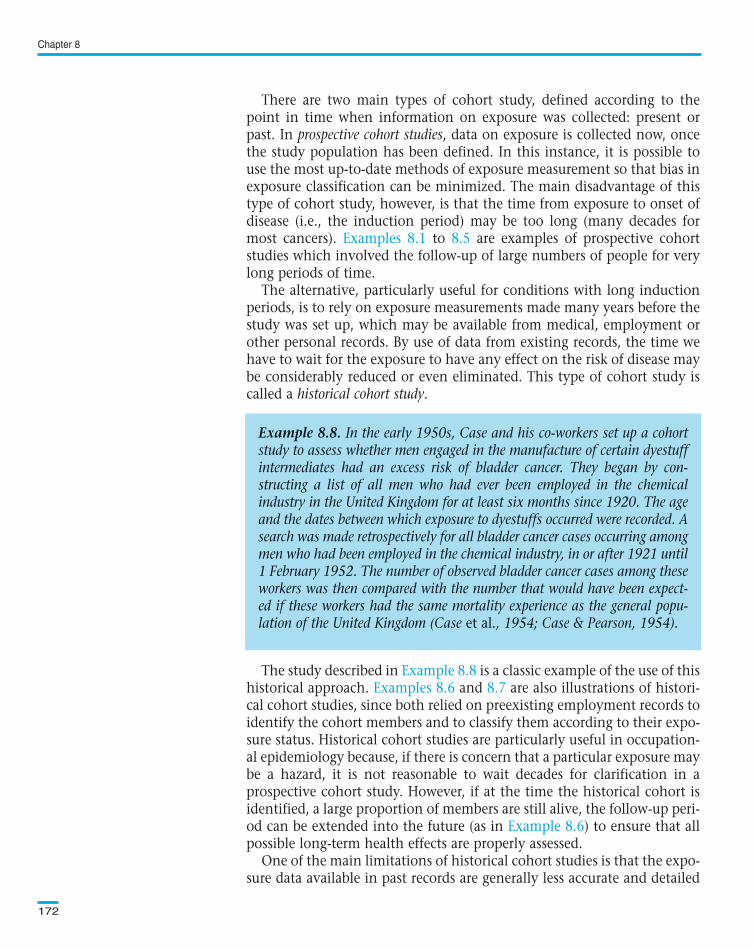
There are two main types of cohort study, defined according to thepoint in time when information on exposure was collected: present orpast. In prospective cohort studies, data on exposure is collected now, oncethe study population has been defined. In this instance, it is possible touse the most up-to-date methods of exposure measurement so that bias inexposure classification can be minimized. The main disadvantage of thistype of cohort study, however, is that the time from exposure to onset ofdisease (i.e., the induction period) may be too long (many decades formost cancers). to are examples of prospective cohortstudies which involved the follow-up of large numbers of people for verylong periods of time.

The alternative, particularly useful for conditions with long inductionperiods, is to rely on exposure measurements made many years before thestudy was set up, which may be available from medical, employment orother personal records. By use of data from existing records, the time wehave to wait for the exposure to have any effect on the risk of disease maybe considerably reduced or even eliminated. This type of cohort study iscalled a historical cohort study.

The study described in is a classic example of the use of thishistorical approach. and are also illustrations of histori-cal cohort studies, since both relied on preexisting employment records toidentify the cohort members and to classify them according to their expo-sure status. Historical cohort studies are particularly useful in occupation-al epidemiology because, if there is concern that a particular exposure maybe a hazard, it is not reasonable to wait decades for clarification in aprospective cohort study. However, if at the time the historical cohort isidentified, a large proportion of members are still alive, the follow-up peri-od can be extended into the future (as in ) to ensure that allpossible long-term health effects are properly assessed.

One of the main limitations of historical cohort studies is that the expo-sure data available in past records are generally less accurate and detailed

Chapter 8

172

Example 8.8. In the early 1950s, Case and his co-workers set up a cohortstudy to assess whether men engaged in the manufacture of certain dyestuffintermediates had an excess risk of bladder cancer. They began by con-structing a list of all men who had ever been employed in the chemicalindustry in the United Kingdom for at least six months since 1920. The ageand the dates between which exposure to dyestuffs occurred were recorded. Asearch was made retrospectively for all bladder cancer cases occurring amongmen who had been employed in the chemical industry, in or after 1921 until1 February 1952. The number of observed bladder cancer cases among theseworkers was then compared with the number that would have been expect-ed if these workers had the same mortality experience as the general popu-lation of the United Kingdom (Case et al., 1954; Case & Pearson, 1954).


Examples 8.1 8.5

Example 8.8Examples 8.6 8.7

Example 8.6

Example 8.8. In the early 1950s, Case and his co-workers set up a cohortstudy to assess whether men engaged in the manufacture of certain dyestuffintermediates had an excess risk of bladder cancer. They began by con-structing a list of all men who had ever been employed in the chemicalindustry in the United Kingdom for at least six months since 1920. The ageand the dates between which exposure to dyestuffs occurred were recorded. Asearch was made retrospectively for all bladder cancer cases occurring amongmen who had been employed in the chemical industry, in or after 1921 until1 February 1952. The number of observed bladder cancer cases among theseworkers was then compared with the number that would have been expect-ed if these workers had the same mortality experience as the general popu-lation of the United Kingdom (Case et al., 1954; Case & Pearson, 1954).


than if they were collected prospectively. Thus, in historical occupationalcohorts, for example, past exposure measurements made in the workingenvironment are rarely available and therefore variables such as workassignment or membership in a union or professional society are general-ly used to classify individual exposure. These proxy variables are, at best,only crude markers of the true exposure levels and the available detail maybe insufficient to address adequately specific research questions. It is, how-ever, unlikely that the accuracy or completeness of these records would bedifferent for those who developed the outcome of interest and those whodid not, since the data were recorded before the individuals developed theoutcome under study, and, in most cases, for reasons totally unrelated tothe investigation. As long as exposure misclassification is independent ofthe outcome status (i.e., is non-differential), it will tend to dilute any trueassociation between the exposure and the outcome (see Sections 2.7 and13.1.2).

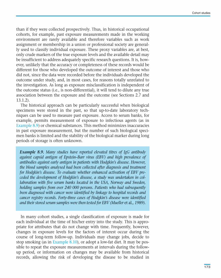
The historical approach can be particularly successful when biologicalspecimens were stored in the past, so that up-to-date laboratory tech-niques can be used to measure past exposure. Access to serum banks, forexample, permits measurement of exposure to infectious agents (as in

) or chemical substances. This method minimizes inaccuraciesin past exposure measurement, but the number of such biological speci-men banks is limited and the stability of the biological marker during longperiods of storage is often unknown.

In many cohort studies, a single classification of exposure is made foreach individual at the time of his/her entry into the study. This is appro-priate for attributes that do not change with time. Frequently, however,changes in exposure levels for the factors of interest occur during thecourse of long-term follow-up. Individuals may change jobs, decide tostop smoking (as in ), or adopt a low-fat diet. It may be pos-sible to repeat the exposure measurements at intervals during the follow-up period, or information on changes may be available from historicalrecords, allowing the risk of developing the disease to be studied in

Cohort studies

173

Example 8.9. Many studies have reported elevated titres of IgG antibodyagainst capsid antigen of Epstein–Barr virus (EBV) and high prevalence ofantibodies against early antigen in patients with Hodgkin’s disease. However,the blood samples analysed had been collected after diagnosis and treatmentfor Hodgkin’s disease. To evaluate whether enhanced activation of EBV pre-ceded the development of Hodgkin’s disease, a study was undertaken in col-laboration with five serum banks located in the USA, Norway and Sweden,holding samples from over 240 000 persons. Patients who had subsequentlybeen diagnosed with cancer were identified by linkage to hospital records andcancer registry records. Forty-three cases of Hodgkin’s disease were identifiedand their stored serum samples were then tested for EBV (Mueller et al., 1989).


Example 8.9

Example 8.10

Example 8.9. Many studies have reported elevated titres of IgG antibodyagainst capsid antigen of Epstein–Barr virus (EBV) and high prevalence ofantibodies against early antigen in patients with Hodgkin’s disease. However,the blood samples analysed had been collected after diagnosis and treatmentfor Hodgkin’s disease. To evaluate whether enhanced activation of EBV pre-ceded the development of Hodgkin’s disease, a study was undertaken in col-laboration with five serum banks located in the USA, Norway and Sweden,holding samples from over 240 000 persons. Patients who had subsequentlybeen diagnosed with cancer were identified by linkage to hospital records andcancer registry records. Forty-three cases of Hodgkin’s disease were identifiedand their stored serum samples were then tested for EBV (Mueller et al., 1989).


relation both to the initial exposure status and to subsequent changes.There may be other reasons for re-assessing the exposure status of the

study subjects, particularly in long-term prospective studies. More refinedmethods of measuring the exposures of interest may become available inthe course of the study or new scientific information about the diseasemay indicate the importance (or desirability) of measuring additional vari-ables that were not measured initially.

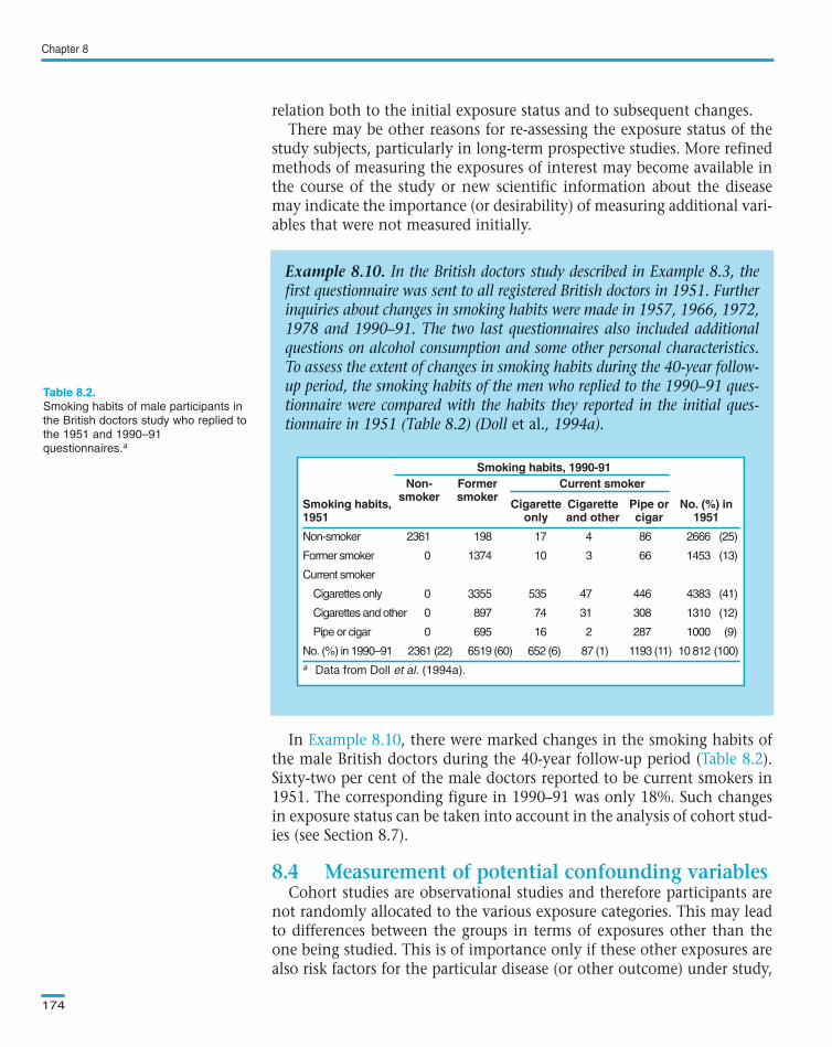
In , there were marked changes in the smoking habits ofthe male British doctors during the 40-year follow-up period ( ).Sixty-two per cent of the male doctors reported to be current smokers in1951. The corresponding figure in 1990–91 was only 18%. Such changesin exposure status can be taken into account in the analysis of cohort stud-ies (see Section 8.7).

Cohort studies are observational studies and therefore participants arenot randomly allocated to the various exposure categories. This may leadto differences between the groups in terms of exposures other than theone being studied. This is of importance only if these other exposures arealso risk factors for the particular disease (or other outcome) under study,

Chapter 8

174

Example 8.10. In the British doctors study described in Example 8.3, thefirst questionnaire was sent to all registered British doctors in 1951. Furtherinquiries about changes in smoking habits were made in 1957, 1966, 1972,1978 and 1990–91. The two last questionnaires also included additionalquestions on alcohol consumption and some other personal characteristics.To assess the extent of changes in smoking habits during the 40-year follow-up period, the smoking habits of the men who replied to the 1990–91 ques-tionnaire were compared with the habits they reported in the initial ques-tionnaire in 1951 (Table 8.2) (Doll et al., 1994a).

Smoking habits, 1990-91Non- Former Current smoker

smoker smokerSmoking habits, Cigarette Cigarette Pipe or No. (%) in1951 only and other cigar 1951

Non-smoker 2361 198 17 4 86 2666 (25)

Former smoker 0 1374 10 3 66 1453 (13)

Current smoker

Cigarettes only 0 3355 535 47 446 4383 (41)

Cigarettes and other 0 897 74 31 308 1310 (12)

Pipe or cigar 0 695 16 2 287 1000 (9)

No. (%) in 1990–91 2361 (22) 6519 (60) 652 (6) 87 (1) 1193 (11) 10 812 (100)

a Data from Doll et al. (1994a).

Smoking habits of male participants in

the British doctors study who replied to

the 1951 and 1990–91

questionnaires.a


Example 8.10Table 8.2

8.4 Measurement of potential confounding variables

Example 8.10. In the British doctors study described in Example 8.3, thefirst questionnaire was sent to all registered British doctors in 1951. Furtherinquiries about changes in smoking habits were made in 1957, 1966, 1972,1978 and 1990–91. The two last questionnaires also included additionalquestions on alcohol consumption and some other personal characteristics.To assess the extent of changes in smoking habits during the 40-year follow-up period, the smoking habits of the men who replied to the 1990–91 ques-tionnaire were compared with the habits they reported in the initial ques-tionnaire in 1951 (Table 8.2) (Doll et al., 1994a).



Non-smoker 2361 198 17 4 86 2666 (25)

Former smoker 0 1374 10 3 66 1453 (13)

Current smoker

Cigarettes only 0 3355 535 47 446 4383 (41)


Pipe or cigar 0 695 16 2 287 1000 (9)

No. (%) in 1990–91 2361 (22) 6519 (60) 652 (6) 87 (1) 1193 (11) 10 812 (100)




Non-smoker 2361 198 17 4 86 2666 (25)

Former smoker 0 1374 10 3 66 1453 (13)

Current smoker

Cigarettes only 0 3355 535 47 446 4383 (41)


Pipe or cigar 0 695 16 2 287 1000 (9)

No. (%) in 1990–91 2361 (22) 6519 (60) 652 (6) 87 (1) 1193 (11) 10 812 (100)


Table 8.2.


i.e., if these exposures are confounding variables. Thus, if we are studyingan occupational exposure in relation to lung cancer, it is necessary to besure that the ‘exposed’ and ‘unexposed’ groups have a similar smokinghistory. If they do not, statistical adjustment for differences in smokingmust be made (see Chapters 13 and 14). In order to carry out this adjust-ment, data on smoking for each individual are required. These data mustbe as accurate as possible and of similar quality to the data on the expo-sure of primary interest.

In historical cohort studies, information on confounding factors is fre-quently missing. This is one of their main limitations. For instance, inmany of the historical occupational cohorts set up to investigate the rela-tionship between asbestos exposure and respiratory cancers, informationon smoking habits was not available. In contrast, the collection of data onpotential confounders can be built into the design of most prospectivecohort studies, except when local or national rates are taken as the unex-posed comparison group.

A major advantage of cohort studies is that it is possible to examine theeffect of a particular exposure on multiple outcomes.

Many cohort studies make use of existing routine surveillance systems toascertain the outcomes of interest. Such systems include cancer registries,death certification and other specialized surveillance systems. They allow trac-ing of study subjects and ascertainment of their outcomes at much lower costthan if it is necessary to personally contact the subjects. However, it is onlypossible to examine outcomes of the type which are recorded routinely bythese systems and according to the way in which they are coded there. This isparticularly important in studies that last for several decades, since majorchanges may be introduced during the study period in the way diseases areascertained and coded by these surveillance systems (see Appendix A.2.2).

When no form of disease surveillance system exists, or when the outcomeof interest is not routinely recorded by them, some form of surveillance ofdisease within the cohort has to be set up. For instance, the ascertainmentof the outcomes of interest may be done through self-administered ques-tionnaires sent regularly to all study subjects, through personal interviews,or by regular physical examination of all members of the cohort.

Regardless of the method chosen to ascertain the outcome(s) of interest,it is vital to ensure that it is used identically for subjects exposed and thosenot exposed. If possible, interviewers and any other persons involved in theascertainment of the outcomes should be kept blind to the exposure statusof the study subjects. Otherwise, there is potential to introduce measure-ment bias (see Section 13.1.2).

Cohort studies focus on disease development. In order for a disease todevelop, it must, of course, be absent at the time of entry into the study. Aninitial examination of the potential study population may be required toidentify and exclude existing cases of disease. Even so, it may still be impos-

Cohort studies

175


8.5 Measurement of outcome(s)


sible to be absolutely certain that all individuals were disease-free at entry tothe study, particularly for conditions with a long latent period (i.e., with along interval from disease initiation to onset of clinical symptoms andsigns). It is therefore usual to exclude disease events occurring during sometime period immediately following entry into the study. For cancer, this isoften the first 2–3 years of follow-up.

The criteria for entry into the cohort must be defined before the start of thestudy in a clear and unambiguous way. Individuals should enter thecohort, and contribute person-time at risk, only after all the entry crite-ria have been satisfied. In most cohort studies, participants will join thecohort at different points in time and therefore the exact date of entry ofeach subject should be recorded.

Methods must be set up at the start of the study to ensure adequate fol-low-up of the study subjects. In general, these involve periodic contactswith the individuals such as home visits, telephone calls or mailed ques-tionnaires. Cohort studies of conditions which have a long inductionperiod require follow-up of a very large number of subjects over manyyears. This is obviously a huge and costly enterprise. To minimize thesedifficulties, many cohorts are defined in terms of membership of a par-ticular group (professional body, occupational pension plan, union,health insurance plan, college alumni), in which the study populationcan be more easily followed. Any routine surveillance system that existsmay be used to trace and follow up the study subjects at much lower costthan if the investigators had to contact them personally.

The criteria for exit from the cohort should also be clearly defined. Adate should be specified as the end of the follow-up period (at least forthe current analysis). For instance, if death is the outcome of interest, thevital status on that date must be ascertained for all cohort members. Allsubjects whose vital status is known at that date should contribute per-son-time at risk until that date (or until their date of death if it occurredearlier). Those whose vital status is not known at that date should be con-sidered as ‘lost to follow-up’ and the last date for which their vital statuswas known should be taken as the end of their contribution to person-time at risk.

It is essential that as high a proportion of people in the cohort as pos-sible is followed up. Some people will migrate, some die and some changeemployment, but every effort should be made to ascertain their out-come(s). All of these factors may be influenced by the exposure and soincomplete follow-up may introduce selection bias (see Section 13.1.1).

The first step in the analysis of a cohort study is to measure the incidence ofdisease (or of any other outcome of interest) in those exposed and in thoseunexposed and compare them.

Chapter 8

176


8.6 Follow-up

8.7 Analysis


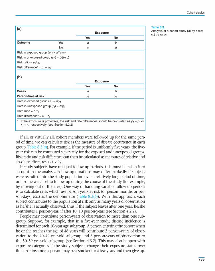
If all, or virtually all, cohort members were followed up for the same peri-od of time, we can calculate risk as the measure of disease occurrence in eachgroup ( ). For example, if the period is uniformly five years, the five-year risk can be computed separately for the exposed and unexposed groups.Risk ratio and risk difference can then be calculated as measures of relative andabsolute effect, respectively.

If study subjects have unequal follow-up periods, this must be taken intoaccount in the analysis. Follow-up durations may differ markedly if subjectswere recruited into the study population over a relatively long period of time,or if some were lost to follow-up during the course of the study (for example,by moving out of the area). One way of handling variable follow-up periodsis to calculate rates which use person-years at risk (or person-months or per-son-days, etc.) as the denominator ( ). With this approach, eachsubject contributes to the population at risk only as many years of observationas he/she is actually observed; thus if the subject leaves after one year, he/shecontributes 1 person-year; if after 10, 10 person-years (see Section 4.2.2).

People may contribute person-years of observation to more than one sub-group. Suppose, for example, that in a five-year study, disease incidence isdetermined for each 10-year age subgroup. A person entering the cohort whenhe or she reaches the age of 48 years will contribute 2 person-years of obser-vation to the 40–49 year-old subgroup and 3 person-years of observation tothe 50–59 year-old subgroup (see Section 4.3.2). This may also happen withexposure categories if the study subjects change their exposure status overtime. For instance, a person may be a smoker for a few years and then give up.

Cohort studies

177

(a)Exposure

Yes No

Outcome Yes a b

No c d

Risk in exposed group (p1) = a/(a+c)

Risk in unexposed group (p0) = b/(b+d)

Risk ratio = p1/p0

Risk differencea = p1 – p0

(b)Exposure

Yes No

Cases a b

Person-time at risk y1 y0

Rate in exposed group (r1) = a/y1

Rate in unexposed group (r0) = b/y0

Rate ratio = r1/r0

Rate differencea = r1 – r0

a If the exposure is protective, the risk and rate differences should be calculated as p0 – p1 orr0 – r1, respectively (see Section 5.2.2)

Analysis of a cohort study (a) by risks;

(b) by rates.


Table 8.3(a)

Table 8.3(b)

(a)Exposure

Yes No

Outcome Yes a b

No c d

Risk in exposed group (p1) = a/(a+c)

Risk in unexposed group (p0) = b/(b+d)

Risk ratio = p1/p0

Risk differencea = p1 – p0

(b)Exposure

Yes No

Cases a b

Person-time at risk y1 y0

Rate in exposed group (r1) = a/y1

Rate in unexposed group (r0) = b/y0

Rate ratio = r1/r0

Rate differencea = r1 – r0

a If the exposure is protective, the risk and rate differences should be calculated as p0 – p1 orr0 – r1, respectively (see Section 5.2.2)

Table 8.3.


In , women who changed their oral contraceptive statusduring the follow-up period would have contributed person-time at risk todifferent exposure categories. For instance, a woman who began using oralcontraceptives at the start of 1978 and stopped by the end of 1984 wouldhave contributed approximately 1.5 person-years to the non-user catego-ry (from the start of the study in mid-1976 to the end of 1977), 7 person-years to the current user category (from the start of 1978 to the end of1984), and 1.5 person-years to the past user category (from the start of1985 until the end of the follow-up in mid-1986). If that woman haddeveloped breast cancer at the end of 1982, her person-time contributionwould have been 1.5 person-years to the non-user category but only 5 per-son-years to the current user category (her person-time contributionwould have been stopped at the time she developed breast cancer).

The outcomes of interest also need to be allocated to the different expo-sure categories. In our previous example, the breast cancer case shouldhave been allocated to the current user category since it occurred duringthe time the woman was contributing person-years to this category. Oncethe person-time at risk and the outcomes are allocated to the relevantexposure categories, it is possible to estimate breast cancer incidence ratesfor each oral contraceptive use category by dividing the number of breast

Chapter 8

178

Example 8.11. The Nurses’ Health Study described in Example 8.5 is acohort study of 121 700 US female registered nurses aged 30–55 years whenthe cohort was established in mid-1976. A total of 1799 newly diagnosedbreast cancer cases were identified during the first 10 years of follow-up frommid-1976 to mid-1986. Analyses were then conducted to investigate therelationship between oral contraceptive use and risk of breast cancer. On thebaseline questionnaire in mid-1976, the following question was asked: “Ifyou are now using or have used oral contraceptives, please indicate intervalsof oral contraceptive use starting from first use and continuing until the pre-sent time. If applicable, please indicate reasons for stopping”. The samequestion was asked on subsequent biennial follow-up questionnaires.

In response to the 1976 questionnaire, 7133 women reported that theywere using oral contraceptives. Responses to the 1978, 1980, and 1982questionnaires showed that 2399, 1168, and 302 women, respectively, werestill using oral contraceptives. In 1984, none of the women were currentusers.

The information given in the 1976 questionnaire was used to classifynurses according to categories of oral contraceptive use (‘non-users’, ‘pastusers’ and ‘current users’) and each nurse started contributing person-time atrisk to that category. Similarly, for each subsequent two-year interval,women contributed additional person-time of follow-up to each updatedreport of oral contraceptive use. The follow-up of women who developedbreast cancer was truncated at the time their breast cancer was diagnosed(Romieu et al., 1989).


Example 8.11

Example 8.11. The Nurses’ Health Study described in Example 8.5 is acohort study of 121 700 US female registered nurses aged 30–55 years whenthe cohort was established in mid-1976. A total of 1799 newly diagnosedbreast cancer cases were identified during the first 10 years of follow-up frommid-1976 to mid-1986. Analyses were then conducted to investigate therelationship between oral contraceptive use and risk of breast cancer. On thebaseline questionnaire in mid-1976, the following question was asked: “Ifyou are now using or have used oral contraceptives, please indicate intervalsof oral contraceptive use starting from first use and continuing until the pre-sent time. If applicable, please indicate reasons for stopping”. The samequestion was asked on subsequent biennial follow-up questionnaires.

In response to the 1976 questionnaire, 7133 women reported that theywere using oral contraceptives. Responses to the 1978, 1980, and 1982questionnaires showed that 2399, 1168, and 302 women, respectively, werestill using oral contraceptives. In 1984, none of the women were currentusers.

The information given in the 1976 questionnaire was used to classifynurses according to categories of oral contraceptive use (‘non-users’, ‘pastusers’ and ‘current users’) and each nurse started contributing person-time atrisk to that category. Similarly, for each subsequent two-year interval,women contributed additional person-time of follow-up to each updatedreport of oral contraceptive use. The follow-up of women who developedbreast cancer was truncated at the time their breast cancer was diagnosed(Romieu et al., 1989).


cancer cases in each category by the corresponding total number of per-son-years ( ).

The results in show that there was no statistically signifi-cant difference in the incidence of breast cancer between ever-users (pastand current users were pooled in this analysis) and never-users of oral con-traceptives.

Most often the exposures we are interested in can be further classifiedinto various levels of intensity. Smokers may be classified by number ofcigarettes smoked per day, oral contraceptive users by total duration ofuse, and occupational exposures by intensity of exposure (often esti-mated indirectly from data on type of job or place of work in the facto-ry) or duration of employment. If various levels of exposure are used inthe cohort, we can examine trends of disease incidence by level of expo-sure. The conclusions from a study are strengthened if there is a trendof increasing risk (or decreasing, if the exposure is protective) withincreasing level of exposure (i.e., if there is an exposure–response rela-tionship).

In , non-users of oral contraceptives were taken as theunexposed baseline category. Rate ratios for each timing and duration cat-egory were calculated by dividing their respective rates by the rate of thebaseline category. Thus, the rate ratio for current users who had used oralcontraceptives for 48 or less months was calculated as 1220 per 100 000pyrs/187 per 100 000 pyrs = 6.52 (95% confidence interval 2.43–17.53)( ). This result suggests that risk might be raised among current

Cohort studies

179

Example 8.12. In Example 8.11, the incidence of breast cancer amongnurses aged 45–49 years at the time of their entry into the cohort wasexamined in relation to use of oral contraceptives.

Oral contraceptive use Total

Ever (current or past use) Never

Cases 204 240 444

Person-years at risk 94 029 128 528 222 557

Rate per 100 000 pyrs 217 187 199

a Data from Romieu et al. (1989)

Rate ratio = 217 per 100 000 pyrs/187 per 100 000 pyrs = 1.16

95% confidence for the rate ratio = 0.96 to 1.40

Rate difference = 217 per 100 000 pyrs – 187 per 100 000 pyrs = 30 per 100 000 pyrs

95% confidence interval for the rate difference = – 8 to 68 per 100 000 pyrs

χ2 = 2.48; 1 d.f.; P=0.12.

(Test statistics and confidence intervals were calculated using the formulae given inAppendix 6.1).

Distribution of breast cancer cases and

person-years at risk among US female

nurses aged 45–49 years at the time

of their entry into the cohort according

to oral contraceptive use.a


Example 8.12Example 8.12

Example 8.13

Table 8.5

Example 8.12. In Example 8.11, the incidence of breast cancer amongnurses aged 45–49 years at the time of their entry into the cohort wasexamined in relation to use of oral contraceptives.



Cases 204 240 444


Rate per 100 000 pyrs 217 187 199






χ2 = 2.48; 1 d.f.; P=0.12.




Cases 204 240 444


Rate per 100 000 pyrs 217 187 199






χ2 = 2.48; 1 d.f.; P=0.12.


Table 8.4.


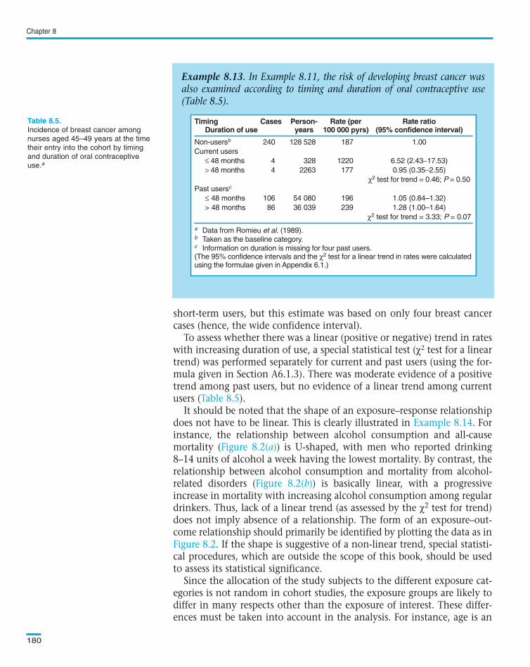
short-term users, but this estimate was based on only four breast cancercases (hence, the wide confidence interval).

To assess whether there was a linear (positive or negative) trend in rateswith increasing duration of use, a special statistical test (χ2 test for a lineartrend) was performed separately for current and past users (using the for-mula given in Section A6.1.3). There was moderate evidence of a positivetrend among past users, but no evidence of a linear trend among currentusers ( ).

It should be noted that the shape of an exposure–response relationshipdoes not have to be linear. This is clearly illustrated in . Forinstance, the relationship between alcohol consumption and all-causemortality ( ) is U-shaped, with men who reported drinking8–14 units of alcohol a week having the lowest mortality. By contrast, therelationship between alcohol consumption and mortality from alcohol-related disorders ( ) is basically linear, with a progressiveincrease in mortality with increasing alcohol consumption among regulardrinkers. Thus, lack of a linear trend (as assessed by the χ2 test for trend)does not imply absence of a relationship. The form of an exposure–out-come relationship should primarily be identified by plotting the data as in

. If the shape is suggestive of a non-linear trend, special statisti-cal procedures, which are outside the scope of this book, should be usedto assess its statistical significance.

Since the allocation of the study subjects to the different exposure cat-egories is not random in cohort studies, the exposure groups are likely todiffer in many respects other than the exposure of interest. These differ-ences must be taken into account in the analysis. For instance, age is an

Chapter 8

180

Example 8.13. In Example 8.11, the risk of developing breast cancer wasalso examined according to timing and duration of oral contraceptive use(Table 8.5).

Timing Cases Person- Rate (per Rate ratioDuration of use years 100 000 pyrs) (95% confidence interval)

Non-usersb 240 128 528 187 1.00

Current users

≤ 48 months 4 328 1220 6.52 (2.43−17.53)

> 48 months 4 2263 177 0.95 (0.35−2.55)

χ2 test for trend = 0.46; P = 0.50

Past usersc

≤ 48 months 106 54 080 196 1.05 (0.84–1.32)

> 48 months 86 36 039 239 1.28 (1.00–1.64)


a Data from Romieu et al. (1989).b Taken as the baseline category.c Information on duration is missing for four past users.(The 95% confidence intervals and the χ2 test for a linear trend in rates were calculatedusing the formulae given in Appendix 6.1.)

Incidence of breast cancer among

nurses aged 45–49 years at the time

their entry into the cohort by timing

and duration of oral contraceptive

use.a


Table 8.5

Example 8.14

Figure 8.2(a)

Figure 8.2(b)

Figure 8.2

Example 8.13. In Example 8.11, the risk of developing breast cancer wasalso examined according to timing and duration of oral contraceptive use(Table 8.5).


Non-usersb 240 128 528 187 1.00

Current users

≤ 48 months 4 328 1220 6.52 (2.43−17.53)

> 48 months 4 2263 177 0.95 (0.35−2.55)


Past usersc

≤ 48 months 106 54 080 196 1.05 (0.84–1.32)

> 48 months 86 36 039 239 1.28 (1.00–1.64)




Non-usersb 240 128 528 187 1.00

Current users

≤ 48 months 4 328 1220 6.52 (2.43−17.53)

> 48 months 4 2263 177 0.95 (0.35−2.55)


Past usersc

≤ 48 months 106 54 080 196 1.05 (0.84–1.32)

> 48 months 86 36 039 239 1.28 (1.00–1.64)



Table 8.5.


important confounding factor of the relationship between oral contracep-tive use and breast cancer, since it is strongly associated with oral contra-ceptive use, and it is in itself an independent risk factor for breast cancer.Thus differences in the age distribution between women in different oralcontraceptive categories may distort the relationship between oral contra-ceptive use and breast cancer incidence. To minimize this potential con-founding effect, we deliberately restricted the analysis in and to a narrow age-stratum (women aged 45–49 years at the time oftheir entry into the cohort). It is, however, possible (and desirable) toobtain summary measures (for all ages combined) that are ‘adjusted’ forage and any other potential confounding variable by using more complex

Cohort studies

181

Example 8.14. In the British doctors study described in Examples 8.3 and8.10, additional questions on alcohol consumption were included in the1978 questionnaire. Doctors were asked about frequency of drinking and, ifthey were regular drinkers (i.e., they drank in most weeks), about how muchthey drank in an average week. By 1991, almost a third of the 12 321 menwho replied had died. The risk of death in men was then examined in rela-tion to self-reported alcohol consumption (Doll et al., 1994b). Some of theresults are shown in Figure 8.2.

Male mortality from various causes by

weekly alcohol consumption: (a) all

causes; (b) conditions known to be

alcohol-related (e.g., cancers of the

liver, mouth, pharynx, oesophagus and

larynx, cirrhosis, alcoholism, and exter-

nal causes); (c) ischaemic heart dis-

ease; (d) other known causes (cere-

brovascular diseases, respiratory dis-

eases, all other cancers not included in

(b), and others). Points and bars are

rates and 95% confidence intervals

adjusted for age, smoking habits and

history of previous disease; the values

are numbers of deaths (reproduced, by

permission of BMJ Publishing Group,

from Doll et al., 1994b).

(a) All causes40

20

0

(b) Alcohol-augmented causes

6

4

2

0

(c) Ischaemic heart disease15

5

10

00 21

Weekly alcohol consumption(British unitsa)

42 63 0 21Weekly alcohol consumption

(British unitsa)

42 63

(d) Other causes30

20

10

0

An

nu

al m

ort

alit

y p

er 1

000

pyr

s

486

170

290

344

387 272237

241

217206235

125111

127 87

585

675 442383

413

344

19

24 3532 26

38

34

a 1 unit = half pint (237 mL) of ordinary beer or one glass (125 mL) of wine or one glass

(62 mL) of sherry or a glass (26 mL) of spirits.


Examples 8.128.13

Example 8.14. In the British doctors study described in Examples 8.3 and8.10, additional questions on alcohol consumption were included in the1978 questionnaire. Doctors were asked about frequency of drinking and, ifthey were regular drinkers (i.e., they drank in most weeks), about how muchthey drank in an average week. By 1991, almost a third of the 12 321 menwho replied had died. The risk of death in men was then examined in rela-tion to self-reported alcohol consumption (Doll et al., 1994b). Some of theresults are shown in Figure 8.2.

(a) All causes40

20

0


6

4

2

0


5

10

00 21



(British unitsa)

42 63

(d) Other causes30

20

10

0

An

nu

al m

ort

alit

y p

er 1

000

pyr

s

486

170

290

344

387 272237

241

217206235

125111

127 87

585

675 442383

413

344

19

24 3532 26

38

34



Figure 8.2.(a) All causes40

20

0


6

4

2

0


5

10

00 21



(British unitsa)

42 63

(d) Other causes30

20

10

0

An

nu

al m

ort

alit

y p

er 1

000

pyr

s

486

170

290

344

387 272237

241

217206235

125111

127 87

585

675 442383

413

344

19

24 3532 26

38

34




statistical methods. Standardization is one of these methods, as we shallsee below. The interpretation of these ‘adjusted summary measures’ is sim-ilar, regardless of the method used. In (and ), rateswere adjusted for age and smoking habits. This means that differences inmortality between the different alcohol consumption categories cannot beexplained by differences in their age or smoking distributions, providedthe measurements of these confounding variables were valid. These issuesare discussed further in Chapters 13 and 14.

Another common method of presenting the results of cohort studies,particularly those based on the disease experience of the general popula-tion as the comparison group, is to calculate standardized mortality (or inci-dence) ratios (see Section 4.3.3). Imagine that a total of 24 deaths fromlung cancer were observed among a cohort of 17 800 male asbestos insu-lators. This observed number (O) is then compared with the number thatwould have been expected (E) if the cohort had the same age-specificmortality rates from lung cancer as the whole male population residentin the same area. Calculations similar to those shown in Section 4.3.3indicate that only seven deaths would have been expected. Thus, theSMR is equal to O/E = 24/7 = 3.4 (or 340 if the SMR is expressed as a per-centage). This measure is, in fact, an age-adjusted rate ratio. In this exam-ple, asbestos insulators were 3.4 times more likely to die from lung can-cer than the entire male population resident in the same area, and thisdifference in mortality is not due to differences in the age-structurebetween the cohort and the general population. A similar approach wasused in . Although this method is often used to adjust forage, it can also be used to adjust for any other confounding variable (e.g.,calendar time, smoking habits). Statistical tests and 95% confidenceintervals for an SMR can be calculated as shown in Sections A6.1.2 andA6.1.3.

Another way of analysing cohort data, which also takes into accountdifferent lengths of follow-up, is to use survival analysis methods. Theseare discussed in Chapter 12.

In a traditional cohort study, all study individuals are subjected to thesame procedures—interviews, health examinations, laboratory measure-ments, etc.—at the time of their entry into the study and throughout thefollow-up period. Alternatively, a cohort may be identified and followedup until a sufficient number of cases develop. More detailed informationis then collected and analysed, but only for the ‘cases’ and for a sampleof the disease-free individuals (‘controls’), not for all members of thecohort. This type of case–control study conducted within a fixed cohortis called a nested case–control study (see Chapter 9). This approach is par-ticularly useful if complex and expensive procedures are being applied.For instance, blood samples for all members of the cohort can be collect-ed at the time of entry and frozen. However, only the blood samples of

Chapter 8

182


Example 8.14 Figure 8.2

Example 8.15

8.8 Cohort studies with nested case–control studies


the cases (i.e., those individuals in the cohort who contract the diseaseunder study) and of a subgroup of individuals who remained disease-free(the controls), are analysed at the end of the follow-up.

In , blood samples were obtained and stored from all42 000 children who participated in the study but the rather complex andexpensive virus tests were carried out only on the serum samples from the16 children who developed the lymphoma and from a sample of about 80selected disease-free members who acted as controls.

Similarly, in nutritional cohort studies, food diaries may be used to mea-sure the subjects’ usual dietary intake. As the coding and analysis of fooddiaries is very labour-intensive, a nested case–control study may be con-ducted in which only the diaries of the cases and of a sample of disease-free members of the cohort (‘controls’) are examined.

Cohort studies

183

Example 8.15. In the occupational cohort described in Example 8.7, themortality experience of 6678 male rubber workers was compared with thatof the 1968 US male population (McMichael et al., 1974). Mortality fromselected causes of death is shown in Table 8.6.

Example 8.16. In 1972, a cohort of 42 000 children was established in theWest Nile District of Uganda in order to investigate the etiological role of theEpstein–Barr virus (EBV) in Burkitt’s lymphoma. A blood sample wasobtained from each child at the time of entry into the study. By the end ofthe follow-up in 1979, 16 new Burkitt’s lymphoma cases had been detectedamong the cohort members. The level of EBV antibodies in the serum sam-ple taken at entry from each of these cases was then compared with the lev-els in the sera of four or five children of the same age and sex who were bledin the neighbourhood at the same time as the Burkitt’s lymphoma case butwho did not develop the disease (‘controls’) (Geser et al., 1982).

Cause of death Observed Expected SMR (%) 95% confidence (ICD-8 code) deaths (O) deaths (E)b (100 ✕ O/E)c interval

All causes 489 524.9 93 85–102

All neoplasms 110 108.9 101 83–122(140–239)

All malignant neoplasms 108 107.3 100 82–120(140–209)

a Data from McMichael et al., 1974).

b Expected deaths calculated on the basis of the US male age-specific death rates, 1968.

c P > 0.10 for all the SMRs shown in the table.

(Test statistics and confidence intervals were calculated using the formulae given in Appendix 6.1.)

Mortality from selected causes of

death among a cohort of male rubber

workers.a


Example 8.16

Example 8.15. In the occupational cohort described in Example 8.7, themortality experience of 6678 male rubber workers was compared with thatof the 1968 US male population (McMichael et al., 1974). Mortality fromselected causes of death is shown in Table 8.6.

Cause of death Observed Expected SMR (%) 95% confidence(ICD-8 code) deaths (O) deaths (E)b (100 ✕ O/E)c interval

All causes 489 524.9 93 85–102

All neoplasms 110 108.9 101 83–122(140–239)





(Test statistics and confidence intervals were calculated using the formulae given inAppendix 6.1.)

Example 8.16. In 1972, a cohort of 42 000 children was established in theWest Nile District of Uganda in order to investigate the etiological role of theEpstein–Barr virus (EBV) in Burkitt’s lymphoma. A blood sample wasobtained from each child at the time of entry into the study. By the end ofthe follow-up in 1979, 16 new Burkitt’s lymphoma cases had been detectedamong the cohort members. The level of EBV antibodies in the serum sam-ple taken at entry from each of these cases was then compared with the lev-els in the sera of four or five children of the same age and sex who were bledin the neighbourhood at the same time as the Burkitt’s lymphoma case butwho did not develop the disease (‘controls’) (Geser et al., 1982).

Cause of death Observed Expected SMR (%) 95% confidence(ICD-8 code) deaths (O) deaths (E)b (100 ✕ O/E)c interval

All causes 489 524.9 93 85–102

All neoplasms 110 108.9 101 83–122(140–239)





(Test statistics and confidence intervals were calculated using the formulae given inAppendix 6.1.)

Table 8.6.


This type of study design and the analysis of its data are discussed fur-ther in Sections 9.3 and 9.5.

The main advantage of cohort studies is that the time sequence betweenexposure to a factor and occurrence of the disease is clearly observed.

Cohort studies may, however, suffer from important bias. Knowledgeof the presence or absence of exposure to a particular factor may affectthe subsequent assessment of disease and introduce measurement bias.This can occur if the decision as to the presence or absence of disease ismade by persons who are aware of the subject’s status with regard to thestudy factor. Cohort studies are also potentially prone to selection biasdue to loss of study subjects. Such losses may occur initially if a portionof the target study population does not participate, or later on as mem-bers of the study population are lost to follow-up. These losses do notnecessarily invalidate the study. However, the investigators should con-sider whether the reasons for loss might have affected the study results.Sometimes it is possible to gather information concerning lost subjects,particularly about whether they left because of illness or death possiblyrelated to the exposures and outcomes under investigation.

As with any other observational study, confounding is a critical issue inthe interpretation of cohort studies. Special statistical techniques can beused to take into account the effect of potential confounding variables,but only if these variables were known at the time of the data collectionand if they were properly measured. If these data were not collected, wehave to judge how much the observed findings are likely to have beenaffected by confounding in the light of all available biological and epi-demiological evidence.

In , uranium miners had significantly elevated mortalityfor cancers at three sites relative to the general population ( ).Before concluding that these raised risks are due to exposures in themines, we need to consider alternative explanations for the observedfindings. A possible explanation for the high risk of lung cancer amongminers is that they were heavier smokers than the general population.No information on smoking habits was available for the miners, but asurvey of 697 men in other Czech uranium mines in 1974 showed that76% were smokers, slightly more than the average (66%) forCzechoslovakian males at that time (see Tomás̆ek et al. (1994)). Theresults from this survey indicate that differences in smoking habits areunlikely to have fully accounted for the estimated five-fold higher lungcancer risk in the miners than in the general population. Moreover,

( ) shows that there was a significant positive trend ofmortality from lung cancer with increasing cumulative exposure toradon. This trend provides considerable support for a true associationbetween exposure to radon and lung cancer. Similar findings have beenfound in other radon-exposed miners.

Chapter 8

184


8.9 Interpretation

Example 8.17Table 8.7

Table8.8 Example 8.18


Cohort studies

185

Example 8.17. A cohort of uranium miners in western Bohemia was identifiedby a retrospective search in 1970 of employment records. Workers were eligiblefor entry into the study if: (a) they started to work underground during 1948–59;(b) they worked there for at least four years; and (c) personnel and employmentrecords were available. A total of 4320 miners were eligible. They were exposedto high radon levels, dust and, in one of the two major mines, also high levelsof arsenic. The mortality experience of these miners up to the end of 1990 (an average of 25 years of follow-up) was then compared with that of the gen-eral population of the former Czechoslovakia. Information on the smoking andalcohol drinking habits of the miners was not available (Tomá̆sek et al., 1993,1994). Mortality in this cohort from selected cancer sites is shown in Table 8.7.

Observed deaths Expected deaths SMR (O/E)b

Cause of death (O) (E)b (95% confidence interval)

Lung cancer 704 138.6 5.08 (4.71–5.47)

Liver cancer 22 13.2 1.67 (1.04–2.52)

Cancer of gallbladder 12 5.3 2.26 (1.16–3.94)and extrahepatic bile ducts

a Data from Tomás̆ek et al. (1993).

b Expected number of deaths (E) calculated using national male age-specific mortality rates for the former Czechoslovakia

Number of observed deaths (O) from

selected cancer sites in the West

Bohemian uranium miners cohort com-

pared with the number expected (E) if

the miners had the same mortality as

the general male population of the for-

mer Czechoslovakia.a

Example 8.18. In the cohort of uranium miners described in Example 8.17, thecumulative exposure to radon gas (and its progeny) was estimated for each miner.The exposure, measured in terms of ‘working level months’ (WLM), was calcu-lated by considering the time spent in each mineshaft in conjunction with about39 000 shaft-specific measurements of radon gas made in 1949–63 (Tomá̆sek etal., 1993). Mortality according to exposure levels is shown in Table 8.8.

Site Cumulative radon exposure (WLM) P-value for <110 110–149 150–209 210–329 ≥≥330 trend

Lung cancer O 86 100 139 161 181 <0.001

O/E b 3.07 3.66 4.98 6.23 8.10

Liver cancer O 7 3 4 5 3 0.57

O/E b 2.70 1.18 1.53 2.04 1.40

Cancer of O 0 2 1 3 6 0.003gallbladder O/E b 0.00 1.92 0.93 3.03 6.73and extrahepaticbile ducts

a Data from Tomás̆ek et al. (1993)

b Expected number of deaths (E) calculated using national male age-specific mortality rates for the former Czechoslovakia.

Number of observed deaths (O) and

standardized mortality ratio (O/E) from

selected cancers by cumulative radon

exposure.a


Example 8.17. A cohort of uranium miners in western Bohemia was identifiedby a retrospective search in 1970 of employment records. Workers were eligiblefor entry into the study if: (a) they started to work underground during 1948–59;(b) they worked there for at least four years; and (c) personnel and employmentrecords were available. A total of 4320 miners were eligible. They were exposedto high radon levels, dust and, in one of the two major mines, also high levelsof arsenic. The mortality experience of these miners up to the end of 1990(an average of 25 years of follow-up) was then compared with that of the gen-eral population of the former Czechoslovakia. Information on the smoking andalcohol drinking habits of the miners was not available (Tomá̆sek et al., 1993,1994). Mortality in this cohort from selected cancer sites is shown in Table 8.7.



Lung cancer 704 138.6 5.08 (4.71–5.47)

Liver cancer 22 13.2 1.67 (1.04–2.52)

Cancer of gallbladder 12 5.3 2.26 (1.16–3.94)and extrahepaticbile ducts


b Expected number of deaths (E) calculated using national male age-specificmortality rates for the former Czechoslovakia



Lung cancer 704 138.6 5.08 (4.71–5.47)

Liver cancer 22 13.2 1.67 (1.04–2.52)

Cancer of gallbladder 12 5.3 2.26 (1.16–3.94)and extrahepaticbile ducts


b Expected number of deaths (E) calculated using national male age-specificmortality rates for the former Czechoslovakia

Table 8.7.

Example 8.18. In the cohort of uranium miners described in Example 8.17, thecumulative exposure to radon gas (and its progeny) was estimated for each miner.The exposure, measured in terms of ‘working level months’ (WLM), was calcu-lated by considering the time spent in each mineshaft in conjunction with about39 000 shaft-specific measurements of radon gas made in 1949–63 (Tomá̆sek etal., 1993). Mortality according to exposure levels is shown in Table 8.8.

Site Cumulative radon exposure (WLM) P-value for<110 110–149 150–209 210–329 ≥≥330 trend

Lung cancer O 86 100 139 161 181 <0.001

O/E b 3.07 3.66 4.98 6.23 8.10


O/E b 2.70 1.18 1.53 2.04 1.40



b Expected number of deaths (E) calculated using national male age-specificmortality rates for the former Czechoslovakia.

Site Cumulative radon exposure (WLM) P-value for<110 110–149 150–209 210–329 ≥≥330 trend

Lung cancer O 86 100 139 161 181 <0.001

O/E b 3.07 3.66 4.98 6.23 8.10


O/E b 2.70 1.18 1.53 2.04 1.40



b Expected number of deaths (E) calculated using national male age-specificmortality rates for the former Czechoslovakia.

Table 8.8.


There was also a positive trend in mortality from gallbladder and extra-hepatic bile duct cancer with increasing levels of cumulative exposure toradon ( ), but there is little supporting evidence in favour of thisfinding from other epidemiological studies, and further investigation isneeded. By contrast, mortality from liver cancer did not increase withcumulative radon exposure, making it unlikely that the excess in the min-ers was caused by radon. No information was available on the alcohol con-sumption of the miners, but they were well paid compared with otherCzech workers and, therefore, it is likely that their alcohol consumptionwas higher than in the general population. They also had a significantexcess of deaths from liver cirrhosis, probably caused by alcohol con-sumption and, for six of the liver cancer deaths, cirrhosis was also men-tioned on the death certificate (Tomás̆ek et al., 1993).

The issues that need to be addressed in interpreting results from cohortstudies are further discussed in Chapter 13.

Chapter 8

186


Table 8.8


Cohort studies

187

Box 8.1. Key issues

• Cohort studies are studies in which subjects are selected on the basis of their

exposure status and then followed up in time. In contrast with intervention stud-

ies, however, the allocation of exposure is not determined by the investigators.

• The main advantages of this type of study are:

1. Exposure is measured before disease onset and is therefore likely to

be unbiased in terms of disease development.

2. Rare exposures can be examined by appropriate selection of study

cohorts.

3. Multiple outcomes (diseases) can be studied for any one exposure.

4. Incidence of disease can be measured in the exposed and unexposed

groups.

• The main disadvantages of this type of study are:

1. They can be very expensive and time-consuming, particularly if con-

ducted prospectively.

2. Changes in exposure status and in diagnostic criteria over time can

affect the classification of individuals according to exposure and dis-

ease status.

3. Ascertainment of outcome may be influenced by knowledge of the

subject’s exposure status (information bias).

4. Losses to follow-up may introduce selection bias.

• Cohort studies in cancer epidemiology generally involve the follow-up of a large

number of individuals for long periods of time. They therefore tend to be very

expensive and time-consuming. Various approaches may be used to reduce the

costs:

1. Use preexisting records (or biological specimens) to identify retro-

spectively a suitable study population and obtain information on the

exposure status of their members (historical cohort study).

2. Use available surveillance systems (e.g., death certification, cancer

registration) to follow up subjects and obtain information on the out-

comes of interest.

3. Use national (or local) rates as the comparison unexposed group.

4. Conduct a nested case–control study.

* The book by Breslow & Day

(1987) provides a very compre-

hensive coverage of the role,

design, analysis and interpreta-

tion of cohort studies in cancer

epidemiology. Some of the mate-

rial is presented at a relatively

advanced level.

* Discussion of the healthy work-

er effect can be found in papers

by Carpenter (1987) and

McMichael (1976).


Box 8.1. Key issues

• Cohort studies are studies in which subjects are selected on the basis of their

exposure status and then followed up in time. In contrast with intervention stud-

ies, however, the allocation of exposure is not determined by the investigators.

• The main advantages of this type of study are:

1. Exposure is measured before disease onset and is therefore likely to

be unbiased in terms of disease development.

2. Rare exposures can be examined by appropriate selection of study

cohorts.

3. Multiple outcomes (diseases) can be studied for any one exposure.

4. Incidence of disease can be measured in the exposed and unexposed

groups.

• The main disadvantages of this type of study are:

1. They can be very expensive and time-consuming, particularly if con-

ducted prospectively.

2. Changes in exposure status and in diagnostic criteria over time can

affect the classification of individuals according to exposure and dis-

ease status.

3. Ascertainment of outcome may be influenced by knowledge of the

subject’s exposure status (information bias).

4. Losses to follow-up may introduce selection bias.

• Cohort studies in cancer epidemiology generally involve the follow-up of a large

number of individuals for long periods of time. They therefore tend to be very

expensive and time-consuming. Various approaches may be used to reduce the

costs:

1. Use preexisting records (or biological specimens) to identify retro-

spectively a suitable study population and obtain information on the

exposure status of their members (historical cohort study).

2. Use available surveillance systems (e.g., death certification, cancer

registration) to follow up subjects and obtain information on the out-

comes of interest.

3. Use national (or local) rates as the comparison unexposed group.

4. Conduct a nested case–control study.

Box 8.1. Key issuesBox 8.1. Key issuesBoxBox 8.1. 8.1. Key Key issues issuesFurther reading


Date post:	11-Feb-2018
Category:	Documents
Upload:	hoangtram
View:	226 times
Download:	0 times

Chapter 8 Cohort studies - · PDF filestudy (e.g., cross-sectional or case–control...

Documents