Chapter 8 The Natural Log and Exponential - University of...

Chapter 8The Natural Log and Exponential

This chapter treats the basic theory of logs and exponentials. It can be studied any time afterChapter 6. You might skip it now, but should return to it when needed.

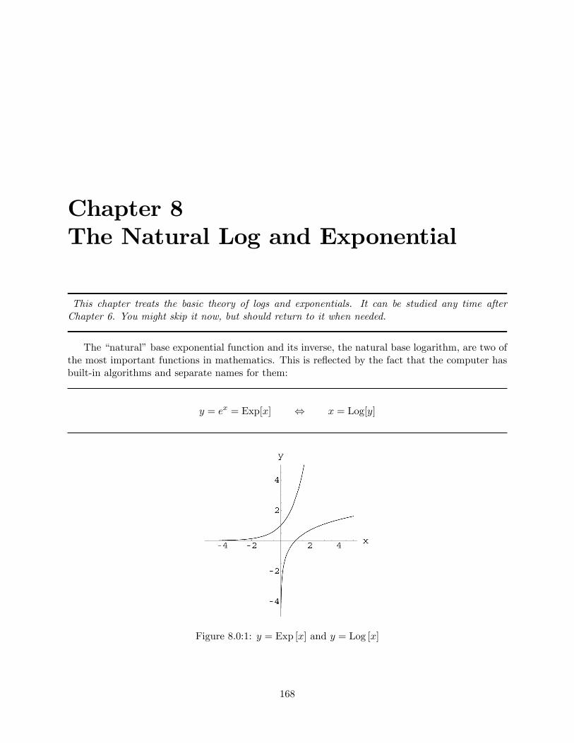
The �natural�base exponential function and its inverse, the natural base logarithm, are two ofthe most important functions in mathematics. This is re�ected by the fact that the computer hasbuilt-in algorithms and separate names for them:

y = ex = Exp[x] , x = Log[y]

Figure 8.0:1: y = Exp [x] and y = Log [x]

168

Chapter 8 - The NATURAL LOG and EXPONENTIAL 169

We did not prove the formulas for the derivatives of logs or exponentials in Chapter 5. Thischapter de�nes the exponential to be the function whose derivative equals itself. No matter wherewe begin in terms of a basic de�nition, this is an essential fact. It is so essential that everythingelse follows from it. We call this the �o¢ cial theory.�

We already know the di¤erentiation rules for log and exponential, and the basic high schoolreview material about logs and exponentials is contained in Chapter 28. The main facts to memorizeare

det

dt = et dLog[s]

ds = 1s

ea � eb = ea+b Log[a� b] = Log[a] + Log[b]&

(ec)t = ec�t Log[ap] = p� Log[a]

Log[et] = t eLog[s] = s; s > 0

Some of the graphical properties of these functions are formulated as limits, comparing them topower functions later in the chapter. Section 8.3 explains these �orders of in�nity�more technicallyand shows how to build more limits from them. The basic limits say

� et goes to in�nity faster than any power as t!1.� Log[t] tends to in�nity slower than any root as t!1.� e�t is positive but tends to zero faster than any reciprocal power as t!1.� Log[s] # �1 as s # 0.

See the the computer programs ExpGth and LogGth in Chapter 28 for an intuitive explanationof these limits.

8.1 The O¢ cial Natural Exponential

One of the most important ways that exponential functions arise in science and mathematics is asthe solution to linear growth and decay laws.

The di¤erential equationdy

dt= k y with a positive constant k represents proportional growth

and with a negative constant represents proportional decay. We have already seen a decay law ofthis form in Newton�s Law of Cooling or the Cool Canary Problem 4.1 and a growth law of thisform in the �rst (false) conjecture of Galileo on the Law of Gravity, Problem 4.2. These laws simplysay, �The rate of change of a quantity is proportional to the amount present.� In Exercise 4.2.1,we solved the di¤erential equation numerically, but now we will be able to solve these problemssymbolically (exactly) in Problems 8.1 and 4.5.


The most noteworthy thing about the formulas in this chapter is this: The dependent variabley appears on both sides of the equation.Something New:

dydt = k y

This is an important di¤erential equation, not just another di¤erentiation formula like the onesin Chapter 6. (Those equations all have explicit functions of the independent variable t on the righthand side, for example, y = 3 t5 ) dy

dt = 15 t4.) It might be worthwhile to contrast this situation

with the �growth form�of a linear function:

Theorem 8.1 The Di¤erential Equation of a Linear Function

For appropriate constants k and Y0, the following are equivalent:

dy

dx= k , y = k x+ Y0

The rate of change of y with respect to x is constant if and only if y varies linearly.

Theorem 8.2 The Di¤erential Equation of an Exponential Function

For appropriate constants k and Y0, the following are equivalent:

1

y

dy

dx= k , y = Y0 e

k x

The rate of change of y is a constant percentage if and only if y varies exponentially. Furthermore,y varies exponentially if and only if Log[y] varies linearly,

y = Y0 ek x , Log[y] = k x+ Log[Y0]

Exercise 5.4 and the PercentGth program (of Chapter 5) show how to �nd an exponentialgiven a �xed percentage change for a �xed change in x. The di¤erential equation 1

ydydx = k simply

says y has the �xed instantaneous percentage change k � 100%.A di¤erential equation tells us how the quantity changes instantaneously. If we also know an

initial value of the quantity, it is intuitively clear that this �start plus change�determines whereyou go, though it may not be entirely clear how it determines it.

Mathematically, a continuous dynamical system is the �operation� of going from the �whereyou start and how you change�to a function of t. We will see that the constant percentage change


system has the solution

y[0] = Y0

dy = k y dt

! y[t] = Y0 ek t; t 2 [0;1)

Without knowing this, we can approximate this �operation�by solving a discrete system that movesin small steps of size �t

y[0] = Y0

y[t+ �t] � y[t] + k y[t] �t! fy[0]; y[�t]; y[2�t]; y[3�t]; � � � g

The solution in this case is y[t] = Y0(1 + �t)t=�t and gives the very fundamental approximation

(1 + �t)t=�t � et

The general idea is called �Euler�s Method�of approximating solutions of initial value problems.We have already seen this idea in several places, beginning with the SecondSIR NoteBook inChapter 2. (Euler�s Method for general systems is studied in Chapter 21.) The point of this sectionis to see that the di¤erential equation gives us a way to work with the function without priorformulas.

You already have an idea of what y = et means, so it may seem a little silly to introduce a�de�nition�for it at this late stage of the game. There may be some gaps in what you know, andwe want a de�nite place to fall back to when the problems get more di¢ cult. For example, laterwe will want to compute ei t, where i =

p�1. Many important functions in higher mathematics

are characterized by their di¤erential equation, so this is the �rst time you will see something thatis quite powerful.

The o¢ cial theory is only important when we get to a question we cannot answer with facts fromhigh school and simple di¤erentiation formulas. What do we mean by e� or even 3

p2? Certainly,

e3 means �multiply e times itself 3 times,� but you cannot multiply e times itself � times - thatmakes no sense. You probably do not want to believe that - because you can use your calculatorfor an approximate answer.

When we use calculators to approximate e� we raise the approximate base e � 2:71828 to theapproximate power � � 3:14159. This implicitly assumes that the yx-button on our calculator iscontinuous in both inputs. In other words, the small errors in both e and � only produce a smallerror in the approximate output to e�. Does your calculator produce six signi�cant digits of e�

when you put 6 digits of accuracy in for e and �? This is a tough question because you have todecide what is exact. Similarly, an approach to exponentials based on

limx!�; y!e

yx = e�


as both y ! e and x ! � is a very di¢ cult way to build a basic theory. It is �natural� in someways but technically too hard. (You will use di¤erentials to prove it later.)

De�nition 8.1 The O¢ cial Natural Exponential FunctionThe function

y = Exp[t]

is o¢ cially de�ned to be the unique solution of the initial value problem

y[0] = 1

dy = y dt

If we use the (unproved) formula for the derivative, we can see that the natural exponentialfunction y[t] = et satis�es this di¤erential equation and initial condition because dydt =

det

dt = et = y

and e0 = 1.The general Euler�s Method is a simple idea once you know the increment approximation from

the De�nition 5.3 of the derivative. When our function is f [x], we write this approximation

f [x+ �x] = f [x] + f 0[x] �x+ " � �x

where the error " � 0 is small when �x � 0 is small. Our function now is y = y[t], so theapproximation becomes

y[t+ �t] = y[t] + y0[t] �t+ " � �t

where " � 0 is small when �t � 0 is small. We do not have a formula for y[t], but we do have thevalue of y[0] = 1 and a formula for y0[t] = y[t] given in terms of y. This gives us

Approximate Solution of y[0] = 1 & dydt = y:

y[t+ �t] = y[t] + y[t] �t+ " � �ty[t+ �t] � y[t] + y[t] �t = y[t](1 + �t) when �t � 0

so

y[�t] � y[0] � (1 + �t) = (1 + �t)y[�t+ �t] � y[�t] � (1 + �t) = (1 + �t)2

y[2�t+ �t] � y[2�t] � (1 + �t) = (1 + �t)2 � (1 + �t) = (1 + �t)3

In general, we see that if y[0] = 1 and dydt = y, then

y[t] � (1 + �t)(t=�t) for t = 0; �t; 2�t; 3�t; � � �


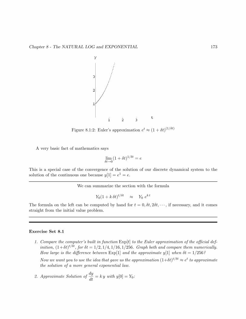
Figure 8.1:2: Euler�s approximation et � (1 + �t)(1=�t)

A very basic fact of mathematics says

lim�t!0

(1 + �t)1=�t = e

This is a special case of the convergence of the solution of our discrete dynamical system to thesolution of the continuous one because y[1] = e1 = e.

We can summarize the section with the formula

Y0(1 + k �t)t=�t � Y0 e

k t

The formula on the left can be computed by hand for t = 0; �t; 2�t; � � � , if necessary, and it comesstraight from the initial value problem.

Exercise Set 8.1

1. Compare the computer�s built in function Exp[t] to the Euler approximation of the o¢ cial def-inition, (1+�t)t=�t, for �t = 1=2; 1=4; 1=16; 1=256. Graph both and compare them numerically.How large is the di¤erence between Exp[1] and the approximate y[1] when �t = 1=256?

Now we want you to use the idea that gave us the approximation (1+�t)t=�t � et to approximatethe solution of a more general exponential law.

2. Approximate Solution ofdy

dt= k y with y[0] = Y0:


(a) Show that y[t] = Y0 (1 + k �t)t=�t (for t = 0; �t; 2�t; 3�t; � � � ) is an approximate solutionto the initial condition and di¤erential equation

y[0] = Y0

dy

dt= k y

(b) Test your approximation numerically and graphically for the special case

y[0] = 3

dy

dt= �2 y

which has the exact solution y[t] = 3Exp[�2 t].

Here is some help with the exercise. First and foremost, recall the microscope approximationof De�nition 5.2 and apply it to the (unknown) function y[t]. Discarding the error term yieldsan approximation:

y[t+ �t] = y[t]+?? + " � �t � y[t]+???

Next, use the fact that y0[t] = k y[t] and substitute this into the microscope approximation,

y[t+ �t] = y[t] � (??)

We know y[0] = Y0, the initial condition. To �nd y[�t], use your approximation

y[�t] � Y0�??y[2�t] � y[�t+ �t] = y[�t]�??y[3�t] � y[2�t+ �t] = y[2�t]�??

Simpli�cation yields the desired result.

3. Log LinearityShow that if y grows at a constant percentage rate with respect to x, then the quantity z =Log[y] is a linear function of x, z = k x+ Z0. Give the value of Z0 in terms of Y0 = y[0].

8.2 e as a �Natural�Base

The number a = e makes y = ax satisfy dydx = y. Similarly, y = e

k x satis�es dydx = k y, and y = b

x

satis�es dydx = k y provided b = e

k.


All exponential bases are not created equal. All exponential functions y = bt satisfy

y[0] = 1

dy

dt/ y

but the base with constant of proportionality 1 is b = e. This makes e the �natural�base from thepoint of view of calculus.

Exercise Set 8.2

1. Let y = bt for an unknown (but �xed) positive constant b. Use the Chain Rule (see Section 6.4)to show that y[t] satis�es

y[0] = 1

dy

dt= k y

What is the value of the constant k?

2. Show that y = ek t satis�es

y[0] = 1

dy

dt= k y

If the constant k is the same as in the �rst part, how much is ek in terms of b?

3. Solve the initial value problem

y[0] = 5

dy

dt= y

4. Solve the initial value problem

y[0] = 5

dy

dt= k y

where k = Log[2]. Show that your solution may also be written as y = 5 � 2t

(See the program ExpEquns.)


The moral of this exercise is this: We could write solutions of initial value problems

y[0] = Y0

dy

dt= k y

as y = Y0 � bt, where b = ek for Log[b] = k; but, for the purposes of calculus, it is �more natural�to write them in the form y = Y0e

k t,

y[0] = Y0

dy = k y dt

! y[t] = Y0 � ek t; t 2 [0;1)

We want you to put this to work in the next problem.

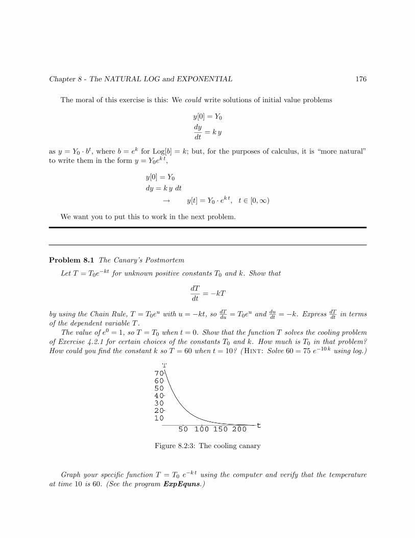
Problem 8.1 The Canary�s Postmortem

Let T = T0e�kt for unknown positive constants T0 and k. Show that

dT

dt= �kT

by using the Chain Rule, T = T0eu with u = �kt, so dTdu = T0e

u and dudt = �k. Express

dTdt in terms

of the dependent variable T .The value of e0 = 1, so T = T0 when t = 0. Show that the function T solves the cooling problem

of Exercise 4.2.1 for certain choices of the constants T0 and k. How much is T0 in that problem?How could you �nd the constant k so T = 60 when t = 10? (Hint: Solve 60 = 75 e�10 k using log.)

Figure 8.2:3: The cooling canary

Graph your speci�c function T = T0 e�k t using the computer and verify that the temperature

at time 10 is 60. (See the program ExpEquns.)


In the saga of the frozen canary, we let the outside temperature be zero. This simpli�es themath (and, of course, freezes the poor dead canary). The next problem has you generalize thelaw of cooling to an arbitrary ambient temperature. We want you to explain why the initial valueproblem:

T [0] = T0

dT

dt= k (Ta � T )

is a reasonable model of temperature adjustment toward ambient - either warming or cooling. Wealso want you to �nd an analytical solution to the model.

Problem 8.2 Newton�s Law of Cooling for Ambient Temperature Ta

Suppose a small object is placed in a large room with constant room temperature Ta - the con-stant ambient temperature. The small inanimate object (that does not heat itself or evaporate,etc.) is placed in the room at a di¤erent initial temperature, T0, and cools or warms toward theroom temperature. This problem helps you formulate Newton�s law of cooling for non-zero ambienttemperature.

1. Let T be the (variable) temperature of your object and t be the time. Choose units of yourliking. The derivative dT

dt represents the instantaneous rate of increase in the temperature.Why?

2. How do we represent warming and cooling in terms of dTdt ?

3. Suppose we put a covered cup of almost boiling water in a normal room, so Ta = 21�Cand T0 = 100�C. Initially, the object cools at a fast rate ( dTdt is a large magnitude negativenumber), while as T approaches Ta = 21, the rate of cooling slows.

(a) What is the value of (Ta� T ) when T = 100? How much �cooling� is happening at thisinstant if dT

dt = k (Ta � T )?(b) How much �cooling� is happening at the instant when T = 22 if dT

dt = k (Ta � T )?

4. Suppose we put a covered cup of almost freezing water in a normal room, so Ta = 21�C andT0 = 0

�C. Initially, the object warms at a fast rate, while as T approaches Ta = 21, the rateof warming slows.

(a) What is the value of (Ta � T ) when T = 0? How much �warming� is happening at thisinstant if dT

dt = k (Ta � T )?(b) How much �warming� is happening at the instant when T = 19 if dT

dt = k (Ta � T )?


5. Use the previous parts of this problem to explain how the initial value problem

T [0] = T0

dT

dt= k (Ta � T )

describes temperature change. Write something like, �The thing that causes the temperatureto change is amount away from ambient temperature of the object : : : and the temperatureadjusts toward ambient. : : : This is because : : :.�

Now that you understand why the initial value problem describes temperature change, solvethe mathematical problem analytically. One approach is to change variables to make the ambientlaw of cooling mathemaitcally the same as the canary law with zero ambient temperature. Thephysical meaning of U in the next problem is �the normalized temperature�or temperature awayfrom ambient.

Problem 8.3 One Solution of T [0] = T0 & dTdt = k (Ta � T )

Let Ta, T0 and k be constants. Let T and U be dependent variables of the independent variablet.

1. Let U = T � Ta or T = U + Ta and show that the following are equivalent initial valueproblems:

T [0] = T0 , U [0] = T0 � Ta

dTdt = k(Ta � T )

dUdt = �k U

2. Show that the solution of

U [0] = U0

dU

dt= �k U

is U [t] = U0 e�k t

3. Let T [t] = U [t] + Ta, where U [t] is the solution to the previous part of this problem andT0 = U0 + Ta. Show that T [t] satis�es

T [0] = T0

dT

dt= k (Ta � T )

and may be written T [t] = Ta + (T0 � Ta) e�k t


4. Prove that T [0] = T0 and limt!1 T [t] = Ta. How could you see the limit directly from thedi¤erential equation?

Another approach to the analytical solution is to just �plug in.�

Problem 8.4 The �Method�of Unknown Constants

Let a, b, and c be constants.

1. (a) Substitute the function y = a+ b ec x into the di¤erential equation

dy

dx= c (y � a)

and show that it is a solution for any value of the constant b.

(b) Substitute the function y = a+ b ec x into the condition

y[0] = 5

and show that you must have b = 5� a.(c) Substitute the function y = a+ b ec x into the initial value problem

y[0] = Y0

dy

dx= c (y � a)

and express b in terms of the constants a, c and Y0.

The story of the fallen tourist in subsection 4.2.2 led to the di¤erential equation

dD

dt= kD

for some positive constant k, where D is the distance an object has fallen and t is time. Thisdi¤erential equation says, �The farther you fall, the faster you go.�in a speci�c way. In a generalsense this is true, but it cannot be speci�cally a linear function of D. We called this Galileo�s �rstconjecture because it gives rise to the Bugs Bunny Law of Gravity: If you don�t look down, youdon�t fall. We want you to show why.

Problem 8.5 Bugs Bunny�s Law of Gravity

How does Bugs�Law say, �The farther you go, the faster you fall?�Prove that an object releasedfrom D = 0 at t = 0 does not fall under the Bugs Bunny Law of Gravity: dDdt = kD, k > 0 constant.(See the program ExpEquns.)


In Problem 21.8, we will look at Wiley Coyote�s Law of Gravity: dDdt = kpD, k > 0 constant.

This law gives a correct prediction to the position of an object falling under gravity, but has thestrange property that, �you don�t fall until you look down.� (It is not a well-posed physical lawbecause of mathematical non-uniqueness.)

Galileo�s simple law d2Ddt2

= g, g a constant, is studied in Exercise 10.2. It is actually simplerthan either Bugs�Law or Wiley�s. And it�s correct, too, in vacuum. The Bungee Diver Projectextends this to falling in air by using Newton�s extension of Galileo�s law.

8.3 Growth of Log, Exp, and Powers

When two functions both tend to in�nity as x tends to in�nity, one may grow �faster.� Thissection shows how to measure of their �order of in�nity�as the limit of their ratio.

Our main aim in this section is to see that logs tend to in�nity �much slower� than powers,whereas exponentials tend to in�nity �much faster�than powers. First, let us think a little aboutthe �eventual growth�of some familiar high school functions.

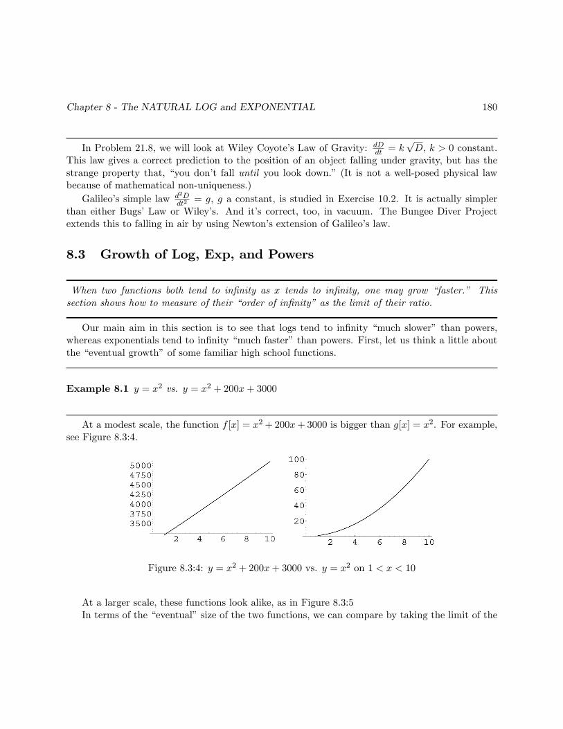
Example 8.1 y = x2 vs. y = x2 + 200x+ 3000

At a modest scale, the function f [x] = x2 +200x+3000 is bigger than g[x] = x2. For example,see Figure 8.3:4.

Figure 8.3:4: y = x2 + 200x+ 3000 vs. y = x2 on 1 < x < 10

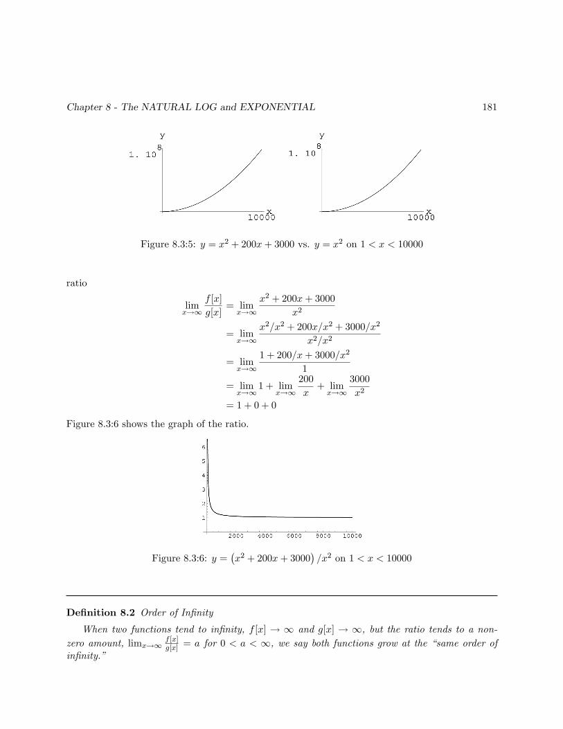
At a larger scale, these functions look alike, as in Figure 8.3:5In terms of the �eventual�size of the two functions, we can compare by taking the limit of the


Figure 8.3:5: y = x2 + 200x+ 3000 vs. y = x2 on 1 < x < 10000

ratio

limx!1

f [x]

g[x]= limx!1

x2 + 200x+ 3000

x2

= limx!1

x2=x2 + 200x=x2 + 3000=x2

x2=x2

= limx!1

1 + 200=x+ 3000=x2

1

= limx!1

1 + limx!1

200

x+ limx!1

3000

x2

= 1 + 0 + 0

Figure 8.3:6 shows the graph of the ratio.

Figure 8.3:6: y =�x2 + 200x+ 3000

�=x2 on 1 < x < 10000

De�nition 8.2 Order of In�nity

When two functions tend to in�nity, f [x] ! 1 and g[x] ! 1, but the ratio tends to a non-zero amount, limx!1

f [x]g[x] = a for 0 < a < 1, we say both functions grow at the �same order of

in�nity.�


In general if f [x] = a xp + �lower power terms�the growth at in�nity is the same as g[x] = xp.Precisely, the limit of the ratio f [x]=g[x] is just the number a. Di¤erent powers, however, grow atdi¤erent rates.

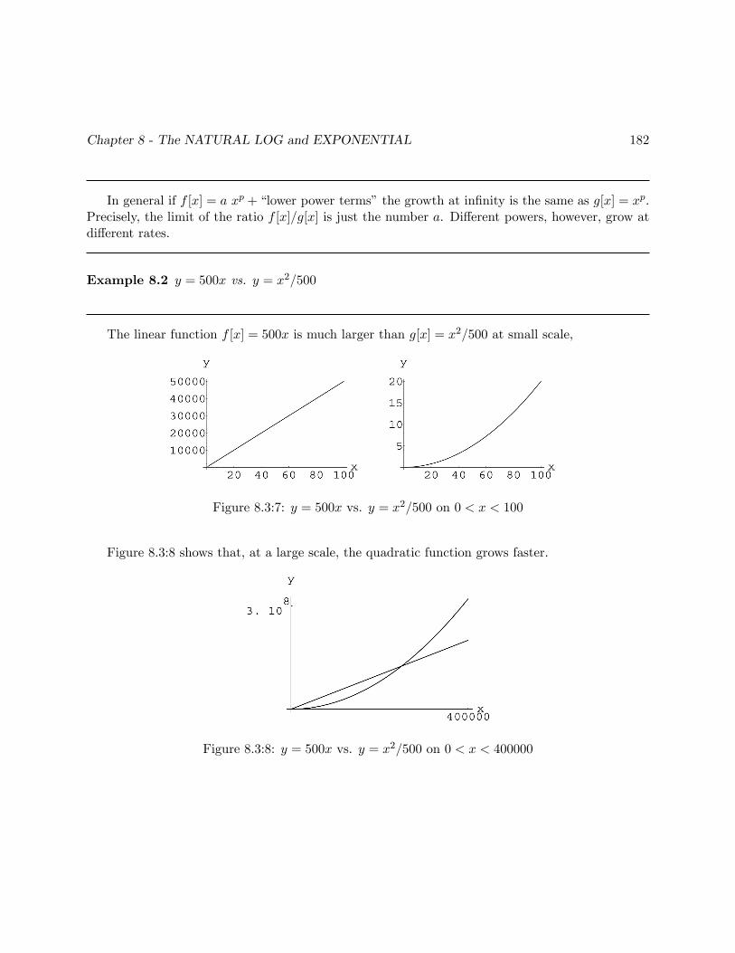
Example 8.2 y = 500x vs. y = x2=500

The linear function f [x] = 500x is much larger than g[x] = x2=500 at small scale,

Figure 8.3:7: y = 500x vs. y = x2=500 on 0 < x < 100

Figure 8.3:8 shows that, at a large scale, the quadratic function grows faster.

Figure 8.3:8: y = 500x vs. y = x2=500 on 0 < x < 400000


The �eventual�size of the two functions can be compared by taking the limit of the ratio

limx!1

f [x]

g[x]= limx!1

500x

x2=500

= limx!1

250000x

x2

= 250000 limx!1

1

x= 0

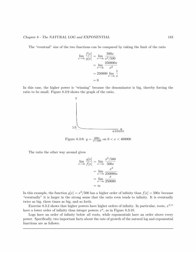
In this case, the higher power is �winning� because the denominator is big, thereby forcing theratio to be small. Figure 8.3:9 shows the graph of the ratio.

Figure 8.3:9: y = 500xx2=500

on 0 < x < 400000

The ratio the other way around gives

limx!1

g[x]

f [x]= limx!1

x2=500

500x

= limx!1

x2

250000x

= limx!1

x

250000=1

In this example, the function g[x] = x2=500 has a higher order of in�nity than f [x] = 500x because�eventually� it is larger in the strong sense that the ratio even tends to in�nity. It is eventuallytwice as big, three times as big, and so forth.

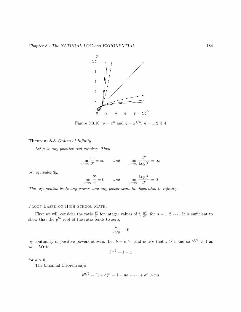
Exercise 8.3.2 shows that higher powers have higher orders of in�nity. In particular, roots, x1=n

have a lower order of in�nity than integer powers xn, as in Figure 8.3:10.Logs have an order of in�nity below all roots, while exponentials have an order above every

power. Speci�cally, two important facts about the rate of growth of the natural log and exponentialfunctions are as follows:


Figure 8.3:10: y = xn and y = x1=n, n = 1; 2; 3; 4

Theorem 8.3 Orders of In�nity

Let p be any positive real number. Then

limt!1

et

tp=1 and lim

t!1

tp

Log[t]=1

or, equivalently,

limt!1

tp

et= 0 and lim

t!1

Log[t]

tp= 0

The exponential beats any power, and any power beats the logarithm to in�nity.

Proof Based on High School Math:

First we will consider the ratio tp

et for integer values of t,np

en , for n = 1; 2; � � � . It is su¢ cient toshow that the pth root of the ratio tends to zero,

n

en=p! 0

by continuity of positive powers at zero. Let b = e1=p, and notice that b > 1 and so b1=2 > 1 aswell. Write

b1=2 = 1 + a

for a > 0.The binomial theorem says

bn=2 = (1 + a)n = 1 + na+ � � �+ an > na


since a > 0, so that en=p = bn > n2a2. Hence, we have

n

en=p<

n

n2a2=

1

na2! 0 as n!1

For continuous values of t > 0, there is always an integer satisfying n � 1 < t � n. For thesevalues, we have

tp

et<

np

en�1= e

np

en! 0

Example 8.3 21=13

There are many other �orders of in�nity�or �orders of in�nitesimal�that we can deduce fromthe basic result given in the preceding theorem. For example, what is

limx!1

2x

x3=?

First, we can write 2 = ek, where k = Log[2]. (Simply take logs of both sides of 2 = ek.) Our limitbecomes

limx!1

ek x

x3=?

for a positive k. (Log[2] = k � 0:693147806.)We consider the kth root of our limit to obtain

limx!1

k

rek x

x3= limx!1

�ek x

x3

�1=k= limx!1

ek x=k

x3=k

= limx!1

ex

xp=1

with p = 3=k, by the theorem. Since positive roots only tend to in�nity when the quantity tendsto in�nity, we have

limx!1

2x

x3=1

Example 8.4 2�1=13 or limx!�1 2x

x3= 0

Consider the limit

limx!�1

2x

x3=?


First, change to natural base.

limx!�1

ek x

x3=?

with k = Log[2] > 0. Next, replace x by u = �x,

limu!+1

e�k u

(�u)3 = � limu!+1

e�k u

u3

Now, notice that the limit is obvious by some arithmetic,

� limu!+1

e�k u

u3= � lim

u!+11

u3 ek u= 0

because both terms in the denominator tend to in�nity. (We can also see this limit by �pluggingin�the limiting values.)

Example 8.5 �13 � 2�1

The limitlim

x!�1x3 2x =?

has one term growing and the other shrinking (2large negative number). Replace x = �u and 2 = ek,for k = Log[2] > 0, so we have

limu!+1

(�u)3 2�u = � limu!+1

u3 2�u

= � limu!+1

u3

2u

= � limu!+1

u3

(ek)u= � lim

u!+1u3

ek u

= 0

since exponentials beat powers to in�nity.Similar tricks reduce various limits to the logarithmic comparison of the Orders of In�nity

Theorem.

Example 8.6 limx#0 xx = 1

We may write x = eLog[x], so xx = ex Log[x] and

limx#0xx = lim

x#0ex Log[x] = elimx#0 x Log[x]

if the last limit exists. This is a fundamental limit which we compute next.


Example 8.7 limx#0 x Log[x] = 0

Replace x = 1=u in the limit, so u! +1 as x # 0, and the limit

limx#0

x Log[x]

becomes

limu!1

1

uLog[

1

u] = lim

u!11

uLog[u�1]

= � limu!1

Log[u]

u= 0

since powers beat logs to in�nity.Now, apply this result to the xx limit,

limx#0xx = elimx#0 x Log[x] = e0 = 1

This limit is a reason to write 00 = 1.

Exercise Set 8.3Use the program In�nities to explore orders of in�nity and compute limits by computer.

1. Ratios of PowersShow that each of the functions g[x] tends to in�nity faster than the corresponding f [x]:

a) g[x] = x5 and f [x] = x3 b) g[x] = x2 and f [x] =px

c) g[x] =px and f [x] = 3

px d) g[x] = x5

10 and f [x] = 10x3

e) g[x] = x2

2 and f [x] = 2px f) g[x] =

px2 and f [x] = 3 3

px

2. Order of PowersLet f [x] = a1xp1 + b1xq1 + c1xr1 and g[x] = a2xp2 + b2xq2 + c2xr2 for positive constants ai, bi,pi, qi, ri. Show that f [x] has a higher order of in�nity than g[x] when the highest power off [x] is greater than the highest power of g[x]. What is the limit of the ratio f [x]=g[x]? Whatis the limit if the highest powers agree?


3. Drill LimitsCompute the limits ( p; k > 0)

a) limx!0 xp Log[x] b) limx!1 x1=x

c) lim�x#0�x1=Log[�x] d) limx!1 xp Log[x]

e) lim�!01+k �� f) lim�#0 �

�+kLog[�]

4. Suppose b > a > 0. Find limx!1 bx

ax

5. Negative? ExponentialsIf the base of an exponential function f [x] = bx satis�es 0 < b < 1, we think of this as a�negative� exponential in the following sense:

(a) Solve for a constant k so that bx = ek x for all x.

(b) Show that k from part (a) is negative when 0 < b < 1.

(c) Show that limx!1 bx = 0 when 0 < b < 1.

6. Use logs to prove the other half of the Orders of In�nity theorem above. If we wish to show

that limx!1xp

Log[x]= 1, then change variables by letting u = Log[x], so x = eu. We show

show instead that

limu!1

(eu)p

u=1

by taking pth roots. Why does this establish the result?

7. All Exponentials Beat All PowersSuppose b > 1 and p > 0. What are the values of the limits

limx!1

bx

xp=? and lim

x!1xp

bx=?

8.4 O¢ cial Properties

The important functional identity ex ey = ex+y follows from the di¤erential equation de�ning theexponential function.

In the Mathematical Background at www.math.uiowa.edu/~stroyan/InfsmlCalculus/FoundationsTOC.htm, we prove a general existence and uniqueness result for continuous dynamical


systems. The proof includes showing that Euler�s approximation converges as the step size �t tendsto zero. Mathematical uniqueness of the solution to an initial value problem is what makes dynam-ical systems deterministic scienti�c models. Uniqueness is really what you are thinking of whenyou say, �The solution of this system models � � � .�Uniqueness is also mathematically important.For now, we will use the following result:

Theorem 8.4 Unique Solution to a Linear Dynamical System

For any real constants Y0 and k, there is a unique real function y[t] de�ned for all real t satisfying

y[0] = Y0

dy

dt= k y

This function can be written y[t] = Y0 ek t.

Simply put, the theorem means that saying y[t] = Y0 ek t is exactly the same thing as saying

y[0] = Y0 anddydt = k y. The theorem assures us in particular that a function Exp[t] of our o¢ cial

de�nition exists. We know intuitively from our experience with programs like SecondSIR andEulerApprox that the computer approximations do converge. The next subsection shows howthe important addition formula for exponentials follows from uniqueness of the solution to ouro¢ cial de�nition.

8.4.1 Proof that ec et = e(c+t)

Let C = Exp[c], and consider the function y[t] = C Exp[t]. We know y[0] = C and by theSuperposition Rule for di¤erentiation that dydt = C Exp[t] = y. This means that y is a solution to

y[0] = C

dy

dt= y

Now consider the function z[t] = Exp[c+ t]. Again, z[0] = Exp[c] = C and the Chain Rule saysdzdt = Exp[c+ t] = z, so z is also a solution to

z[0] = C

dz

dt= z

This is the same dynamical system, written with a di¤erent letter. Uniqueness means that bothy[t] and z[t] are the same function

Exp[c] Exp[t] = Exp[c+ t]


and proves the functional identity of the natural exponential function.Our new de�nition causes us a technical problem. We know how to compute rational powers of

e. We want to show that the new de�nition extends what we already know.

Problem 8.6 Let e be the number Exp[1], that is, the value of the solution of the dynamical systemat time 1.

1. Show that e2 = Exp[2].

2. Show that e1=3 = Exp[1=3] by letting a = Exp[1=3] and computing a� a� a.

3. Show that eq = Exp[q] for any rational q = m=n.

8.5 Projects

8.5.1 Numerical Computation of dat

dt

There are two small Projects that will help you understand the natural base. The �rst has you usethe computer to directly compute the derivative of bt. You will see that this leads to

dbt

dt/ bt

but it does not give an obvious value to the constant of proportionality. However, you can ex-periment with your computations and �nd the value of b that makes this constant one. This isb = e � 2:71828 � � � .

8.5.2 The Canary Resurrected - Cooling Data

The second mathematical project in that chapter asks you to compare some actual cooling data withthe prediction of Newton�s law of cooling. It is an interesting scienti�c project for you to measurethis yourself and we believe that you can do better than the �rst student data we present if youwish to try. (We are not sure if the students warmed the cup before they started measurements.You will see how this shows up in their data.)

Date post:	29-May-2019
Category:	Documents
Upload:	dotram
View:	226 times
Download:	0 times

Chapter 8 The Natural Log and Exponential - University of...

Documents