Chapter 9 Aggregate Demand and Economic Fluctuations
Chapter 9: Aggregate Demand and Economic Fluctuations............................................... 2 1. The Business Cycle......................................................................................................... 2
1.1 What Happens During the Business Cycle ............................................................... 2 1.2 A Stylized Business Cycle ........................................................................................ 5 1.3 The Downturn Side of the Story ............................................................................... 7 Discussion Questions ...................................................................................................... 7
2. Macroeconomic Modeling and Aggregate Demand ....................................................... 8 2.1 Simplifying Assumptions.......................................................................................... 9 2.2 Output, Income, and Aggregate Demand ................................................................. 9 2.3 The Problem of Leakages ....................................................................................... 11 2.4 The Classical Solution to Leakages ........................................................................ 13 Discussion Questions .................................................................................................... 17
3. The Keynesian Model ................................................................................................... 17 3.1 Consumption........................................................................................................... 17 Math Review Box: Graphing with a Slope-Intercept Equation .................................... 20 News In Context: Americans’ Savings Rate Declines in 2005..................................... 22 3.2 Investment............................................................................................................... 22 3.3 The Aggregate Demand Schedule .......................................................................... 23 3.4 The Possibility of Unintended Investment.............................................................. 26 3.5 Movement to Equilibrium in the Keynesian Model ............................................... 28 3.6 The Problem of Persistent Unemployment ............................................................. 29 3.7 The Multiplier ......................................................................................................... 31 Discussion Questions .................................................................................................... 33
Chapter 9: Aggregate Demand and Economic Fluctuations
What if, in a sophisticated contemporary economy like that in the U.S., many people were to suddenly decide to cut way back on buying things? You may have heard it said that it is people’s duty to keep on spending, in order to keep the economy humming and employment high. National leaders have been known to exhort people to keep on buying things if it looks like the economy might be turning towards a recession. When environmentalists or people concerned about the harms of consumerism talk about cutting back on wasteful consumption, their opponents often respond that this would be “bad for the economy” because it would lead to a reduced level of economic activity and an increase in unemployment. How can we understand these various arguments? 1. The Business Cycle Part III of this textbook focuses in particular on the goal of economic stabilization – that is, keeping unemployment and inflation at acceptable levels over the business cycle. For the moment, we will set aside consideration of our two other goals – the goal of improvement in true living standards and the goal of maintaining the ecological, social, and financial sustainability of a national economy – in order to focus only on stabilization. As we will see, one crucial key to understanding macroeconomics is comprehending how the amount that people want to spend overall (or “aggregate demand,” as we called it in Chapter 1) influences, and is influenced by, other macroeconomic variables. One of the key debates in macroeconomic policy is between Keynesians, who believe that aggregate demand needs active guidance if the economy is to be stable, and the Classicals, who believe that aggregate demand can take care of itself.
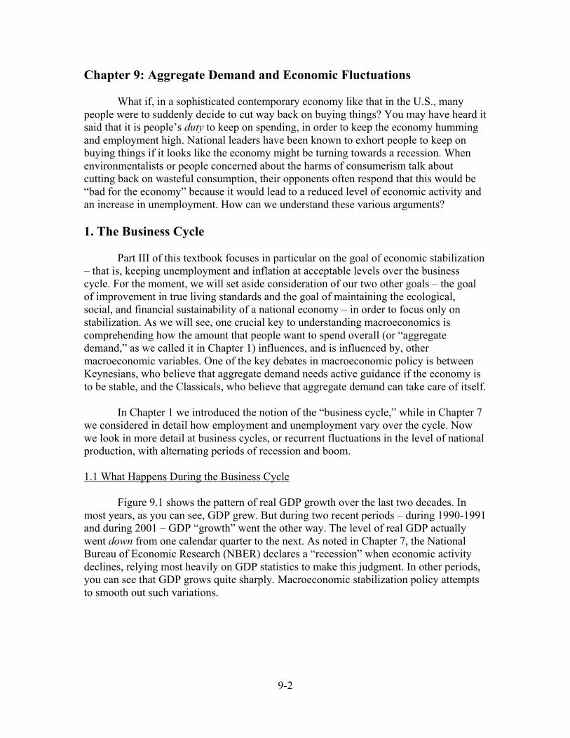
In Chapter 1 we introduced the notion of the “business cycle,” while in Chapter 7 we considered in detail how employment and unemployment vary over the cycle. Now we look in more detail at business cycles, or recurrent fluctuations in the level of national production, with alternating periods of recession and boom. 1.1 What Happens During the Business Cycle Figure 9.1 shows the pattern of real GDP growth over the last two decades. In most years, as you can see, GDP grew. But during two recent periods – during 1990-1991 and during 2001 – GDP “growth” went the other way. The level of real GDP actually went down from one calendar quarter to the next. As noted in Chapter 7, the National Bureau of Economic Research (NBER) declares a “recession” when economic activity declines, relying most heavily on GDP statistics to make this judgment. In other periods, you can see that GDP grows quite sharply. Macroeconomic stabilization policy attempts to smooth out such variations.
9-3
5000
6000
7000
8000
9000
10000
11000
1985
1986
1988
1990
1992
1993
1995
1997
1999
2000
2002
2004
GD
P
(Bill
ions
of C
hain
ed 2
000
Dol
lars
)
Year1990-1991
2001
Figure 9.1 U.S. Real GDP 1985-2005 and NBER Recessions
In recent decades, the U.S. has experienced two recessions, as defined by the National Bureau of Economics Research. During these periods, real GDP fell.
Source: BEA quarterly data and NBER As we discuss the ins and outs of stabilization policy, there are two “stylized facts” that you need to keep in mind. Economists call these “stylized facts” because, while they form a very important base for the way we think about the economy, they are not always literally true.1
Stylized Fact #1: During an economic downturn or contraction, unemployment rises, while in a recovery or expansion, unemployment falls. This is fairly easy to understand, since, when production in an economy is falling, it would seem natural to assume that producers need fewer workers – because they are producing fewer goods. Similarly, in an expansion, unemployment falls. Some economists like to think of this relationship as being determined by an equation they call Okun’s Law. In the early 1960s economist Arthur M. Okun estimated that a 1% drop in the unemployment rate was associated with an approximately 3% boost to real GDP. The equation for Okun’s “Law” has been estimated many times since then, and in many different variations, and is best regarded as a rule of thumb rather than a “law.”
1 For example, you might usefully rely on the “stylized fact” that you normally eat sandwiches for lunch when you do your grocery shopping. But if you get the stomach flu, or a friend comes by with take-out, your “fact” is no longer literally true.
9-4
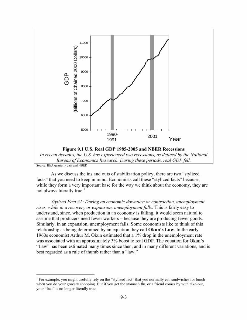
Okun’s “Law”: an empirical inverse relationship between the unemployment rate and rapid (above-average) real GDP growth.2 We can see some strong evidence of this inverse relationship between output
growth and employment by comparing Figure 9.1 with Figure 9.2, which shows the unemployment rate from 1985-2005, including the two recessions that occurred during this period. As output turns down in Figure 9.1, unemployment shoots up dramatically in Figure 9.2. The inverse relation, however, is not perfect. The unemployment rate continued to rise even after GDP started to rise again, after the last two recessions – the “jobless recoveries” discussed in Chapter 7. But, for most of Part III of this book, we will assume that rising GDP is associated with increased employment.
0
2
4
6
8
10
12
198519
8619
8719
8819
8919
9019
9119
9219
9319
9419
9519
9619
9719
9819
9920
0020
0120
0220
0320
0420
051990-1991
2001 Year
Une
mpl
oym
ent R
ate
Figure 9.2 U.S. Unemployment Rate 1985-2005 and NBER Recessions
During the two most recent recessions, unemployment shot up sharply. Source: BLS monthly data and NBER
Stylized Fact #2: An economic recovery or expansion, if it is very strong, tends to leads to an increase in the inflation rate. During a downturn or contraction, pressure on inflation eases off (and inflation may fall or even become negative). The reasoning behind this result is that, as an economy “heats up,” producers come more and more into competition with each other for a limited supply of raw materials, labor, and so on. Prices and wages tend to be bid up, and inflation results or intensifies. In a slump, this upwards pressure on prices slackens, or even reverses, so inflation may be lower or even, in some 2 In a “jobless recovery,” real GDP growth is slow (below average) so that it does not create jobs fast enough to counter-act the normal increase in the labor force and decrease in labor demand due to increased output per worker.
9-5
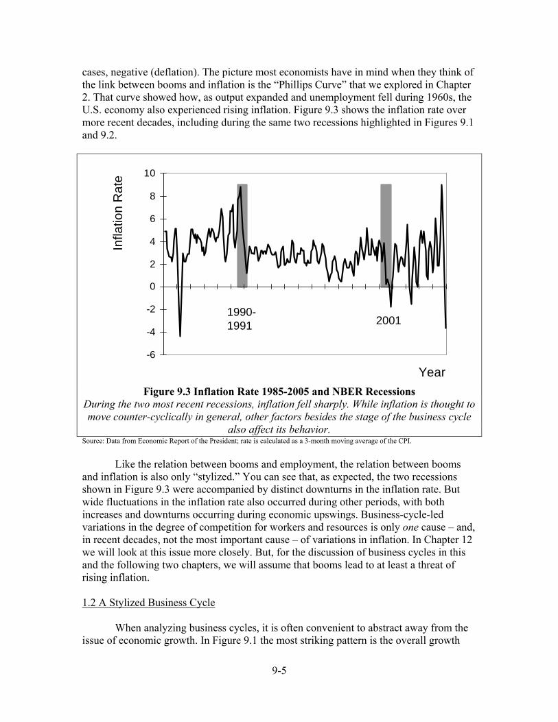
cases, negative (deflation). The picture most economists have in mind when they think of the link between booms and inflation is the “Phillips Curve” that we explored in Chapter 2. That curve showed how, as output expanded and unemployment fell during 1960s, the U.S. economy also experienced rising inflation. Figure 9.3 shows the inflation rate over more recent decades, including during the same two recessions highlighted in Figures 9.1 and 9.2.
-6
-4
-2
0
2
4
6
8
10
Year
Infla
tion
Rat
e
1990-1991 2001
Figure 9.3 Inflation Rate 1985-2005 and NBER Recessions
During the two most recent recessions, inflation fell sharply. While inflation is thought to move counter-cyclically in general, other factors besides the stage of the business cycle
also affect its behavior. Source: Data from Economic Report of the President; rate is calculated as a 3-month moving average of the CPI. Like the relation between booms and employment, the relation between booms and inflation is also only “stylized.” You can see that, as expected, the two recessions shown in Figure 9.3 were accompanied by distinct downturns in the inflation rate. But wide fluctuations in the inflation rate also occurred during other periods, with both increases and downturns occurring during economic upswings. Business-cycle-led variations in the degree of competition for workers and resources is only one cause – and, in recent decades, not the most important cause – of variations in inflation. In Chapter 12 we will look at this issue more closely. But, for the discussion of business cycles in this and the following two chapters, we will assume that booms lead to at least a threat of rising inflation. 1.2 A Stylized Business Cycle When analyzing business cycles, it is often convenient to abstract away from the issue of economic growth. In Figure 9.1 the most striking pattern is the overall growth
9-6
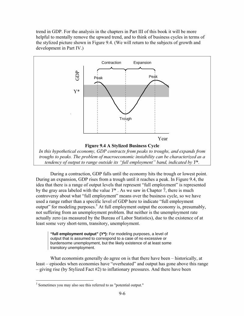
trend in GDP. For the analysis in the chapters in Part III of this book it will be more helpful to mentally remove the upward trend, and to think of business cycles in terms of the stylized picture shown in Figure 9.4. (We will return to the subjects of growth and development in Part IV.)
Year
Peak Peak
Trough
Contraction Expansion
GD
P
Y*
Figure 9.4 A Stylized Business Cycle
In this hypothetical economy, GDP contracts from peaks to troughs, and expands from troughs to peaks. The problem of macroeconomic instability can be characterized as a
tendency of output to range outside its “full employment” band, indicated by Y*. During a contraction, GDP falls until the economy hits the trough or lowest point. During an expansion, GDP rises from a trough until it reaches a peak. In Figure 9.4, the idea that there is a range of output levels that represent “full employment” is represented by the gray area labeled with the value Y* . As we saw in Chapter 7, there is much controversy about what “full employment” means over the business cycle, so we have used a range rather than a specific level of GDP here to indicate “full employment output” for modeling purposes.3 At full employment output the economy is, presumably, not suffering from an unemployment problem. But neither is the unemployment rate actually zero (as measured by the Bureau of Labor Statistics), due to the existence of at least some very short-term, transitory, unemployment.
“full employment output” (Y*): For modeling purposes, a level of output that is assumed to correspond to a case of no excessive or burdensome unemployment, but the likely existence of at least some transitory unemployment.
What economists generally do agree on is that there have been – historically, at
least – episodes when economies have “overheated” and output has gone above this range – giving rise (by Stylized Fact #2) to inflationary pressures. And there have been
3 Sometimes you may also see this referred to as "potential output."
9-7
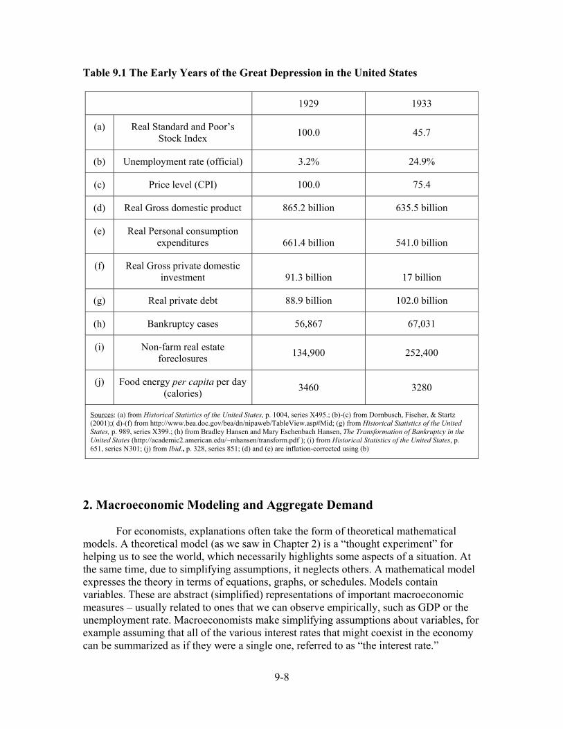
episodes when economies have fallen into troughs, with (due to Stylized Fact #1) unacceptable levels of unemployment. In this stylized representation of the business cycle, the goal of stabilization policy is to keep an economy in the grey area, avoiding the threats of inflation and unemployment. 1.3 The Downturn Side of the Story It will take all of this chapter and the next three to build up a workable theory of the business cycle! Because this is a large and complex topic, we need to take things one step at a time. We will start by looking at the case of economic downturns. The biggest downturn in U.S. history was, of course, the Great Depression. Production dropped dramatically from 1929 to 1930 and unemployment soared, topping out at 25%. Not only were times bad – they stayed bad. Unemployment stayed in the double-digits all through the 1930s. Nor was the Great Depression just a U.S. phenomenon. Most of this country’s major trading partners were also hard hit. Table 9.1 presents some additional descriptive data about the falloff in economic activity in the U.S., and resulting hardships, during the Great Depression. Notice that in our stylized business cycle in Figure 9.4 there is no scale on the “year” axis. The timing of the cycle is not regular or predictable, so that economists in the early years of the Depression differed on how to interpret it. Most economists in the 1930s, trained in the Classical school, reassured public leaders that this sort of cycle was merely to be expected. They saw the economy as being in the “trough” stage, but it would soon start to expand again. In the long run, they assured officials, the economy would recover by itself, as it had recovered from other downturns in the past. In response, British economist John Maynard Keynes quipped that “in the long run, we are all dead.” In 1936 he presented a theory for how economies can fall into recessions and stay there for a long time – and some ideas about how public policy might help economies get out of the trough more quickly. We start our detailed study of business cycle theory with models that illustrate Classical and Keynesian theories concerning recession and depressions. Discussion Questions 1. Do you know anyone who experienced the Great Depression of the 1930s? What do
they say about the effects of that economic stagnation on their lives and those of their friends and neighbors?
2. Do you know what phase of the business cycle we were in two or three years ago? Is
the U.S. economy currently in a recession or an expansion?
9-8
Table 9.1 The Early Years of the Great Depression in the United States
1929 1933
(a) Real Standard and Poor’s Stock Index 100.0 45.7
(b) Unemployment rate (official) 3.2% 24.9%
(c) Price level (CPI) 100.0 75.4
(d) Real Gross domestic product 865.2 billion 635.5 billion
(e) Real Personal consumption expenditures 661.4 billion 541.0 billion
(f) Real Gross private domestic investment 91.3 billion 17 billion
(g) Real private debt 88.9 billion 102.0 billion
(h) Bankruptcy cases 56,867 67,031
(i) Non-farm real estate foreclosures 134,900 252,400
(j) Food energy per capita per day (calories) 3460 3280
Sources: (a) from Historical Statistics of the United States, p. 1004, series X495.; (b)-(c) from Dornbusch, Fischer, & Startz (2001);( d)-(f) from http://www.bea.doc.gov/bea/dn/nipaweb/TableView.asp#Mid; (g) from Historical Statistics of the United States, p. 989, series X399.; (h) from Bradley Hansen and Mary Eschenbach Hansen, The Transformation of Bankruptcy in the United States (http://academic2.american.edu/~mhansen/transform.pdf ); (i) from Historical Statistics of the United States, p. 651, series N301; (j) from Ibid., p. 328, series 851; (d) and (e) are inflation-corrected using (b)
2. Macroeconomic Modeling and Aggregate Demand For economists, explanations often take the form of theoretical mathematical models. A theoretical model (as we saw in Chapter 2) is a “thought experiment” for helping us to see the world, which necessarily highlights some aspects of a situation. At the same time, due to simplifying assumptions, it neglects others. A mathematical model expresses the theory in terms of equations, graphs, or schedules. Models contain variables. These are abstract (simplified) representations of important macroeconomic measures – usually related to ones that we can observe empirically, such as GDP or the unemployment rate. Macroeconomists make simplifying assumptions about variables, for example assuming that all of the various interest rates that might coexist in the economy can be summarized as if they were a single one, referred to as “the interest rate.”
9-9
Mathematical models relate these variables together using algebraic formulas, graphs, and/or tables in such as way as to make clear how these variables affect each other, according to the theorist’s understanding. 2.1 Simplifying Assumptions
At the end of Chapter 5, you learned about the traditional macroeconomic model in which the economy is portrayed in a simplified form involving four sectors and a streamlined set of activities. Household expenditures on consumption, business expenditures on investment, government spending, and exchange with the foreign sector by way of net exports were said to add up to GDP. While the traditional model already abstracts away from many things – for example, from household and government investment – the models of aggregate demand we will now develop simplify even further:
• For all of the models in Part III of this book, we will assume that the full-employment output level does not grow. In designing models, it is often useful to separate out different issues into different models. Chapters in Part IV of this text examine economic growth, and ignore business cycles. In Part III, we take an opposite but complementary approach, concentrating on cycles and abstracting away from growth.
• For the remainder of the present chapter (only), we assume that the only actors in the economy are households and businesses. We also assume that all income in the economy goes to households, in return for the labor or capital services they provide.4 We will reintroduce the government and foreign sectors in later chapters.
• For the remainder of the present chapter (only), we concentrate on explaining the difference between the Classical and Keynesian theories about the behavior of economies that face a threat of recession and rising unemployment due to (potentially) insufficient aggregate demand. We will leave consideration of booms and inflationary pressures for later chapters.
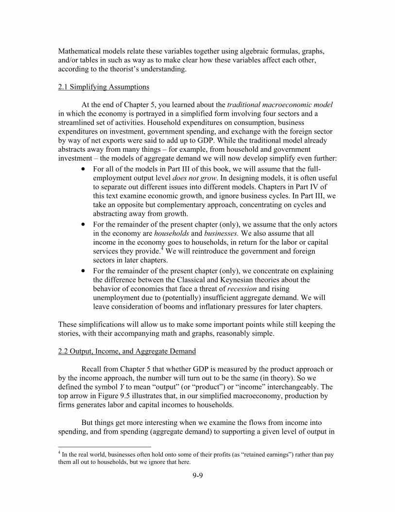
These simplifications will allow us to make some important points while still keeping the stories, with their accompanying math and graphs, reasonably simple. 2.2 Output, Income, and Aggregate Demand Recall from Chapter 5 that whether GDP is measured by the product approach or by the income approach, the number will turn out to be the same (in theory). So we defined the symbol Y to mean “output” (or “product”) or “income” interchangeably. The top arrow in Figure 9.5 illustrates that, in our simplified macroeconomy, production by firms generates labor and capital incomes to households.
But things get more interesting when we examine the flows from income into spending, and from spending (aggregate demand) to supporting a given level of output in
4 In the real world, businesses often hold onto some of their profits (as “retained earnings”) rather than pay them all out to households, but we ignore that here.
9-10
the economy. A macroeconomy is in an equilibrium situation when output, income and spending are all in balance—when they are linked in an unbroken chain, each supported by each other at the equilibrium level, as illustrated in Figure 9.5.
Output (Y)
Income(Y)
Spending(Aggregate Demand or AD)
Spending stimulates firms to produce
Production generates incomes
Incomes give actors the ability to spend
Figure 9.5 The Output-Income-Spending Flow of an Economy in Equilibrium A macroeconomy is said to be in equilibrium when the incomes that arise from
production give rise to a level of spending that, in turn, stimulates producers to produce the original level of output.
But the Keynesian model turns on the idea that spending or aggregate demand,
which we will denote by the symbol AD, may (at least temporarily) fall out of balance with the other flows. Aggregate demand in the economy depends on the spending behavior of the economic actors in the economy. Households make consumption spending decisions, and together the household sector generates an aggregate level of consumption, C. We assume that households always consume at the level they plan to, given their incomes—that what they end up spending is always exactly equal to what they intended to spend. But for firms, the situation can be more complicated, as we will see as this chapter progresses. Business firms invest, and we will call the amount they plan to invest over the course of a year II for intended investment. Since the only actors we are looking at right now are households and businesses, we begin our modeling of aggregate demand with the equation:
AD = C + II AD is the level of spending that would result if people are able to follow their plans.
9-11
aggregate demand (AD) (traditional macro model, with no government and a closed economy) : what households and firms intend to spend on consumption and investment: AD = C + II
But, you might ask, didn’t we say earlier (and in Chapter 5) that “output,”
“income,” and “spending” are all three just different ways of approaching GDP? The basic identity of the traditional macro model (simplified to two sectors) implies that
Y = C + I
This is true, too. Y = C + I is an accounting identity. At the end of any year, when actual flows of output, income, and spending are tallied up in the national accounts, the spending by households and businesses must (in an economy with no government or foreign sector) be equal to GDP. This equation is true in the same way that, in business accounting, net worth is defined as equal to assets minus liabilities. The equation AD = C + II, in contrast, represents something different. It is what is called a behavioral equation. It is made up by economists for modeling purposes – we do not have a national agency that looks into business leaders’ minds and measures their intentions! You will work with both of the equations above later in this chapter. The accounting identity involves the actual level of investment, while the behavioral equation involves the level of planned, desired, or intended investment. While households always actually spend what they have intended to spend (so we do not need a separate symbol for "intended consumption"), Y and AD will only be the same if actual investment (I) is equal to intended investment (II).
behavioral equation: in contrast to an accounting identity, a behavioral equation reflects a theory about the behavior of one or more economic agents or sectors. The variables in the equation may or may not be observable.
Note that Y = C + I is an accounting identity, which represents the actual level of aggregate spending that in fact occurs. AD = C + II is a behavioral equation, which describes the levels of spending that economic actors plan, whether or not this planned level of spending matches what is actually achieved.
The link from income (Y) to spending (AD) is the potential weak link in the chain illustrated in Figure 9.4. This is because the people who get the income do not just automatically go out and spend it all. This creates the problem of leakages. 2.3 The Problem of Leakages The household sector, we have assumed, receives all the income in the economy. Households spend some of this income on consumption goods, and save the rest, according to the equation:
S = Y − C
9-12
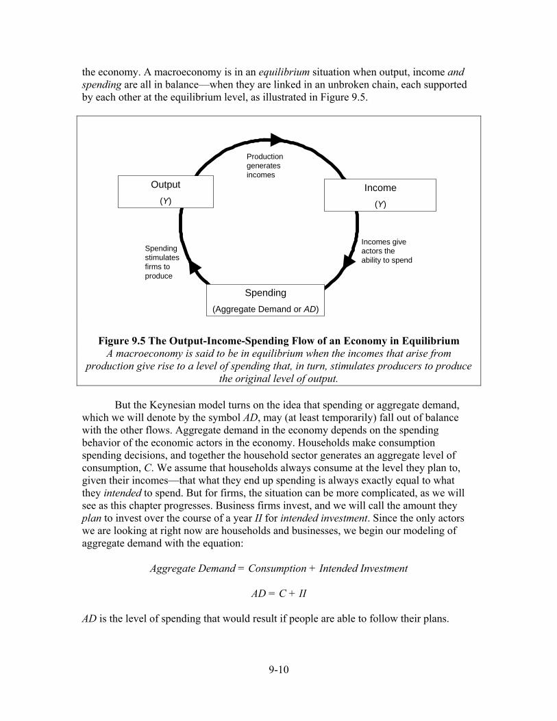
where S is the aggregate level of saving. Saving is considered a “leakage” from the output-income-spending cycle, because it represents income that is not spent on currently produced goods and services. This is illustrated in Figure 9.6, which shows that some funds are diverted from the income-spending part of the cycle.
Production generates income tohouseholds
saving (S)
leakage
intended investment ( II )injection
firms decide how much to invest
households decide how much to consume and save
Output (Y)
Spending (AD)
Income (Y)
consumption (C)?Sufficient to sustain output at a steady level
Figure 9.6 The Output-Income-Spending Flow with Leakages and Injections When households save rather than spend part of their incomes,
funds are diverted from the income-spending flow. When firms spend on investment goods, this creates a flow into the spending stream.
The other side of the coin, however, is that businesses need funds if they are going to be able to buy investment goods. (Remember, we have assumed that they do not hold onto any of the income they receive, but pass it all along to households as wages, profits, interest, or rents.) In our simple model we assume that firms must borrow from the savings put away by households in order to be able to finance investment projects. You can think of households depositing theirs savings in banks, with firms taking out loans from the banks to buy structures or equipment. In this way, firms can shoot funds back into the spending stream in the form of investment. This “injection” of spending through investment is also illustrated in Figure 9.6. If the amount that households want to save is equal to the amount that firms want to invest, then these two flows will balance each other out:
In equilibrium: leakages = injections
S = II
9-13
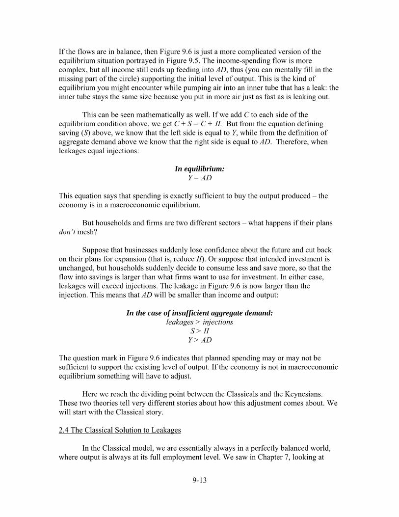
If the flows are in balance, then Figure 9.6 is just a more complicated version of the equilibrium situation portrayed in Figure 9.5. The income-spending flow is more complex, but all income still ends up feeding into AD, thus (you can mentally fill in the missing part of the circle) supporting the initial level of output. This is the kind of equilibrium you might encounter while pumping air into an inner tube that has a leak: the inner tube stays the same size because you put in more air just as fast as is leaking out.
This can be seen mathematically as well. If we add C to each side of the equilibrium condition above, we get C + S = C + II. But from the equation defining saving (S) above, we know that the left side is equal to Y, while from the definition of aggregate demand above we know that the right side is equal to AD. Therefore, when leakages equal injections:
In equilibrium:
Y = AD This equation says that spending is exactly sufficient to buy the output produced – the economy is in a macroeconomic equilibrium. But households and firms are two different sectors – what happens if their plans don’t mesh? Suppose that businesses suddenly lose confidence about the future and cut back on their plans for expansion (that is, reduce II). Or suppose that intended investment is unchanged, but households suddenly decide to consume less and save more, so that the flow into savings is larger than what firms want to use for investment. In either case, leakages will exceed injections. The leakage in Figure 9.6 is now larger than the injection. This means that AD will be smaller than income and output:
In the case of insufficient aggregate demand:
leakages > injections S > II
Y > AD The question mark in Figure 9.6 indicates that planned spending may or may not be sufficient to support the existing level of output. If the economy is not in macroeconomic equilibrium something will have to adjust. Here we reach the dividing point between the Classicals and the Keynesians. These two theories tell very different stories about how this adjustment comes about. We will start with the Classical story. 2.4 The Classical Solution to Leakages In the Classical model, we are essentially always in a perfectly balanced world, where output is always at its full employment level. We saw in Chapter 7, looking at
9-14
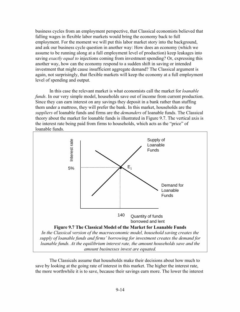
business cycles from an employment perspective, that Classical economists believed that falling wages in flexible labor markets would bring the economy back to full employment. For the moment we will put this labor market story into the background, and ask our business cycle question in another way: How does an economy (which we assume to be running along at a full employment level of production) keep leakages into saving exactly equal to injections coming from investment spending? Or, expressing this another way, how can the economy respond to a sudden shift in saving or intended investment that might cause insufficient aggregate demand? The Classical argument is again, not surprisingly, that flexible markets will keep the economy at a full employment level of spending and output. In this case the relevant market is what economists call the market for loanable funds. In our very simple model, households save out of income from current production. Since they can earn interest on any savings they deposit in a bank rather than stuffing them under a mattress, they will prefer the bank. In this market, households are the suppliers of loanable funds and firms are the demanders of loanable funds. The Classical theory about the market for loanable funds is illustrated in Figure 9.7. The vertical axis is the interest rate being paid from firms to households, which acts as the “price” of loanable funds.
Quantity of funds borrowed and lent
Inte
rest
rate
140
5%
Supply of Loanable Funds
Demand for Loanable Funds
E1
Figure 9.7 The Classical Model of the Market for Loanable Funds
In the Classical version of the macroeconomic model, household saving creates the supply of loanable funds and firms’ borrowing for investment creates the demand for loanable funds. At the equilibrium interest rate, the amount households save and the
amount businesses invest are equated. The Classicals assume that households make their decisions about how much to save by looking at the going rate of interest in this market. The higher the interest rate, the more worthwhile it is to save, because their savings earn more. The lower the interest
9-15
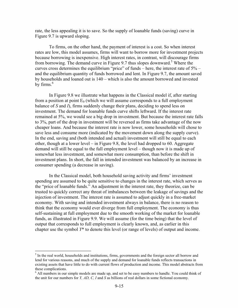
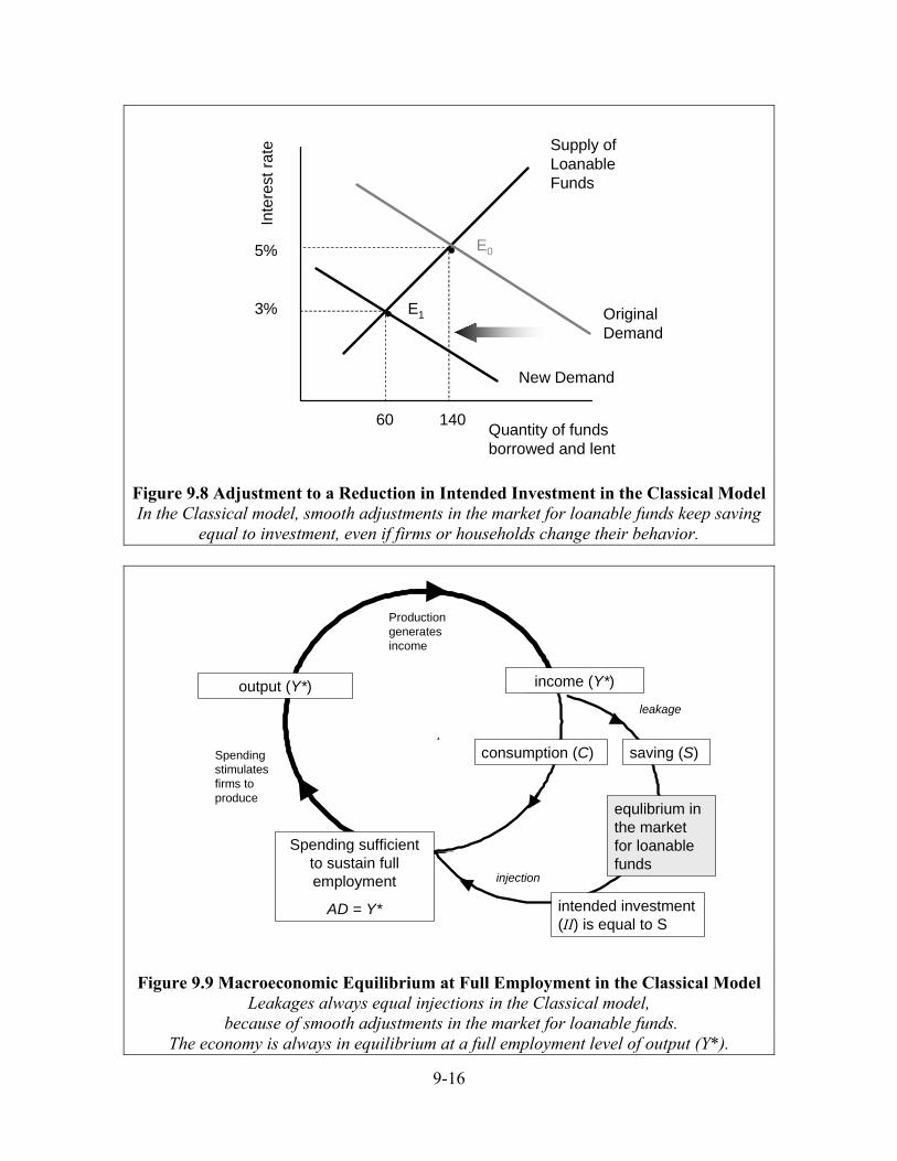
rate, the less appealing it is to save. So the supply of loanable funds (saving) curve in Figure 9.7 is upward sloping. To firms, on the other hand, the payment of interest is a cost. So when interest rates are low, this model assumes, firms will want to borrow more for investment projects because borrowing is inexpensive. High interest rates, in contrast, will discourage firms from borrowing. The demand curve in Figure 9.7 thus slopes downward.5 Where the curves cross determines the equilibrium “price” of funds – here, the interest rate of 5% – and the equilibrium quantity of funds borrowed and lent. In Figure 9.7, the amount saved by households and loaned out is 140 – which is also the amount borrowed and invested by firms.6 In Figure 9.8 we illustrate what happens in the Classical model if, after starting from a position at point E0 (which we will assume corresponds to a full employment balance of S and I), firms suddenly change their plans, deciding to spend less on investment. The demand for loanable funds curve shifts leftward. If the interest rate remained at 5%, we would see a big drop in investment. But because the interest rate falls to 3%, part of the drop in investment will be reversed as firms take advantage of the now cheaper loans. And because the interest rate is now lower, some households will chose to save less and consume more (indicated by the movement down along the supply curve). In the end, saving and (both intended and actual) investment will still be equal to each other, though at a lower level – in Figure 9.8, the level had dropped to 60. Aggregate demand will still be equal to the full employment level – though now it is made up of somewhat less investment, and somewhat more consumption, than before the shift in investment plans. In short, the fall in intended investment was balanced by an increase in consumer spending (a decrease in saving). In the Classical model, both household saving activity and firms’ investment spending are assumed to be quite sensitive to changes in the interest rate, which serves as the “price of loanable funds.” An adjustment in the interest rate, they theorize, can be trusted to quickly correct any threat of imbalances between the leakage of savings and the injection of investment. The interest rate is assumed to adjust quickly in a free-market economy. With saving and intended investment always in balance, there is no reason to think that the economy would ever diverge from full employment. The economy is thus self-sustaining at full employment due to the smooth working of the market for loanable funds, as illustrated in Figure 9.9. We will assume (for the time being) that the level of output that corresponds to full employment is clearly known, and, as earlier in this chapter use the symbol Y* to denote this level (or range of levels) of output and income.
5 In the real world, households and institutions, firms, governments and the foreign sector all borrow and lend for various reasons, and much of the supply and demand for loanable funds reflects transactions in existing assets that have little to do with current flows of production and income. This model abstracts from these complications. 6 All numbers in our simple models are made up, and set to be easy numbers to handle. You could think of the unit for our numbers for Y, AD, C, I and S as billions of real dollars in some fictional economy.
9-16
Quantity of funds borrowed and lent
Inte
rest
rate
140
5%
Supply of Loanable Funds
Original Demand
E1
New Demand
60
3%
E0
Figure 9.8 Adjustment to a Reduction in Intended Investment in the Classical Model In the Classical model, smooth adjustments in the market for loanable funds keep saving
equal to investment, even if firms or households change their behavior.
leakage
injection
Production generates income
Spending stimulates firms to produce
saving (S)
equlibrium in the market for loanable funds
intended investment (II) is equal to S
output (Y*)
consumption (C)
income (Y*)
Spending sufficient to sustain full employment
AD = Y*
Figure 9.9 Macroeconomic Equilibrium at Full Employment in the Classical Model
Leakages always equal injections in the Classical model, because of smooth adjustments in the market for loanable funds.
The economy is always in equilibrium at a full employment level of output (Y*).
9-17
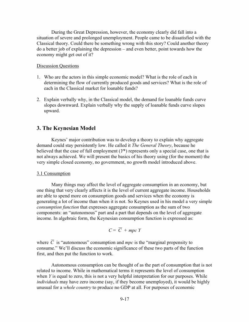
During the Great Depression, however, the economy clearly did fall into a situation of severe and prolonged unemployment. People came to be dissatisfied with the Classical theory. Could there be something wrong with this story? Could another theory do a better job of explaining the depression – and even better, point towards how the economy might get out of it? Discussion Questions 1. Who are the actors in this simple economic model? What is the role of each in
determining the flow of currently produced goods and services? What is the role of each in the Classical market for loanable funds?
2. Explain verbally why, in the Classical model, the demand for loanable funds curve
slopes downward. Explain verbally why the supply of loanable funds curve slopes upward.
3. The Keynesian Model Keynes’ major contribution was to develop a theory to explain why aggregate demand could stay persistently low. He called it The General Theory, because he believed that the case of full employment (Y*) represents only a special case, one that is not always achieved. We will present the basics of his theory using (for the moment) the very simple closed economy, no government, no growth model introduced above. 3.1 Consumption
Many things may affect the level of aggregate consumption in an economy, but one thing that very clearly affects it is the level of current aggregate income. Households are able to spend more on consumption goods and services when the economy is generating a lot of income than when it is not. So Keynes used in his model a very simple consumption function that expresses aggregate consumption as the sum of two components: an “autonomous” part and a part that depends on the level of aggregate income. In algebraic form, the Keynesian consumption function is expressed as:
C = C + mpc Y where C is “autonomous” consumption and mpc is the “marginal propensity to consume.” We’ll discuss the economic significance of these two parts of the function first, and then put the function to work.
Autonomous consumption can be thought of as the part of consumption that is not related to income. While in mathematical terms it represents the level of consumption when Y is equal to zero, this is not a very helpful interpretation for our purposes. While individuals may have zero income (say, if they become unemployed), it would be highly unusual for a whole country to produce no GDP at all. For purposes of economic
9-18
analysis, it is more helpful to think about it as something that, when it changes, shifts the consumption schedule up or down (as we will see below). Some like to think of it as a minimum level of income that people feel required to spend for survival. Others see it as reflecting the amount of consumption spending people will undertake no matter what their current incomes are, reflecting their long-term plans, their commitments and habits, and their place in the community.
But of course, much of consumption does reflect current income and its changes. The name “mpc” comes from the fact that this term reflects the number of additional dollars of consumption spending that occur for every additional dollar of aggregate income. Using the notation “∆” (which is read as the Greek letter delta) to mean “change in,” the marginal propensity to consume can be expressed as:
mpc = ∆C /∆Y
= (the change of C resulting from a change in Y) ÷ (the change in Y)
In the example which follows, we will use an mpc of 8/10 or 0.8. This means that for every additional $10 of aggregate income in the economy, the household sector spends and additional $8 on consumption. Logically the mpc should be no greater than one unless people spend more than their incomes. An mpc of about 0.8 has been the standard, historically, in Keynesian modeling exercises – though such a value may not correspond well to actual data on consumption in every time period. (See News In Context, below.) Recall that, since, S = Y – C, any income not spent by the household sector is saved. Parallel to the mpc, a “marginal propensity to save” can be defined as:
mps = ∆S /∆Y = 1 – mpc
The last line shows that if households spend 80% of additional income, or $8 out of an additional $10 in income, then they must save 20% (= 1 – 80%), or $2 out of $10. That is, if the mpc is 0.8, the mps must be 0.2.
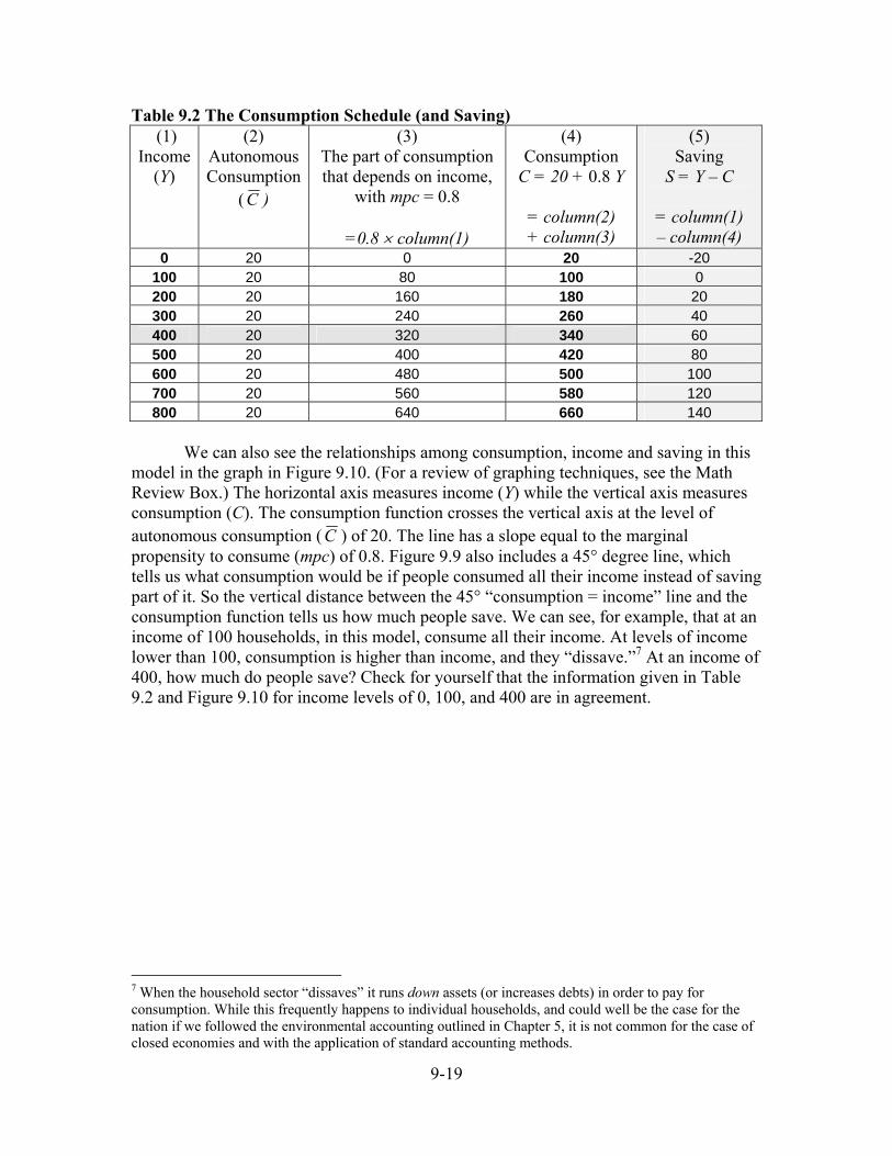
If we assign number values to the parameters C and mpc, we can express the relation between income and consumption stated in the consumption function by a schedule, as in Table 9.2. Various incomes levels are shown in Column (1). We will, for now, set autonomous consumption equal to 20 (as shown in Column (2)). With an mpc set equal to 0.8, Column (3) shows how to calculate the second component of the consumption function. Adding together the autonomous and income-related components yields total consumption, shown in Column (4). We also show in Column (5), for later reference, the implied level of saving. For example, the shaded row indicates that when income is 400, C = 20 + 0.8 (400) = 20 + 320 = 340. Saving is calculated as 400 – 340 = 60. Consumption and saving both steadily rise as income rises.
9-19
Table 9.2 The Consumption Schedule (and Saving) (1)
Income (Y)
(2) Autonomous Consumption
(C )
(3) The part of consumption that depends on income,
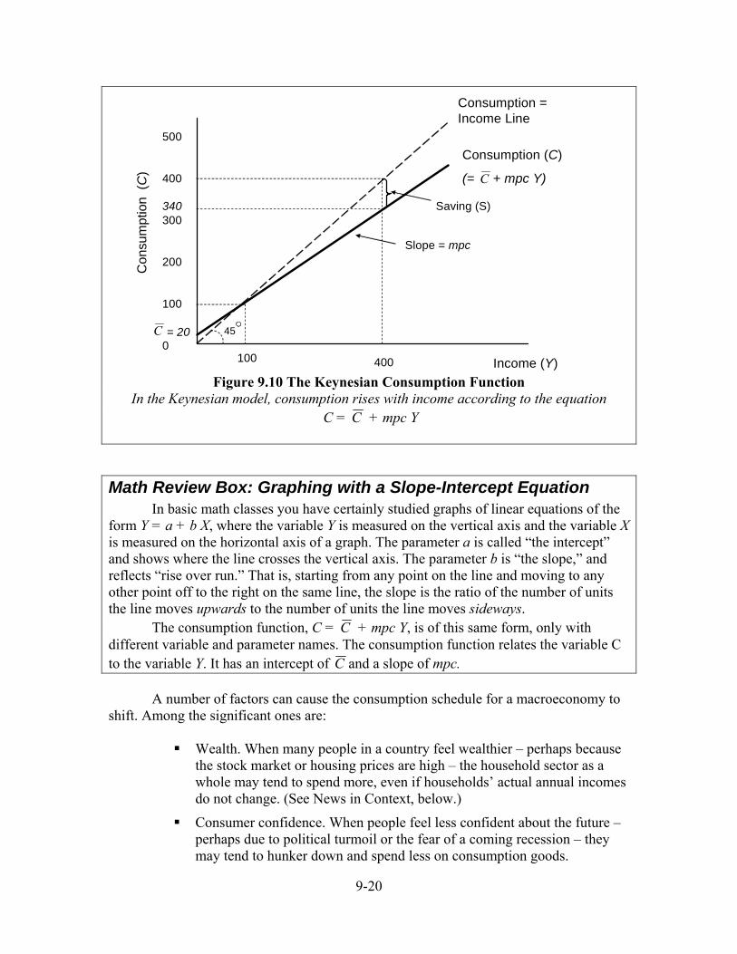
We can also see the relationships among consumption, income and saving in this
model in the graph in Figure 9.10. (For a review of graphing techniques, see the Math Review Box.) The horizontal axis measures income (Y) while the vertical axis measures consumption (C). The consumption function crosses the vertical axis at the level of autonomous consumption (C ) of 20. The line has a slope equal to the marginal propensity to consume (mpc) of 0.8. Figure 9.9 also includes a 45° degree line, which tells us what consumption would be if people consumed all their income instead of saving part of it. So the vertical distance between the 45° “consumption = income” line and the consumption function tells us how much people save. We can see, for example, that at an income of 100 households, in this model, consume all their income. At levels of income lower than 100, consumption is higher than income, and they “dissave.”7 At an income of 400, how much do people save? Check for yourself that the information given in Table 9.2 and Figure 9.10 for income levels of 0, 100, and 400 are in agreement.
7 When the household sector “dissaves” it runs down assets (or increases debts) in order to pay for consumption. While this frequently happens to individual households, and could well be the case for the nation if we followed the environmental accounting outlined in Chapter 5, it is not common for the case of closed economies and with the application of standard accounting methods.
9-20
45
Consumption (C)
(= + mpc Y)
Income (Y)
Con
sum
ptio
n (C
)
Consumption = Income Line
400
Saving (S)
100
C
500
400
300
200
100
0= 20
340
C
Slope = mpc
Figure 9.10 The Keynesian Consumption Function
In the Keynesian model, consumption rises with income according to the equation C = C + mpc Y
Math Review Box: Graphing with a Slope-Intercept Equation In basic math classes you have certainly studied graphs of linear equations of the form Y = a + b X, where the variable Y is measured on the vertical axis and the variable X is measured on the horizontal axis of a graph. The parameter a is called “the intercept” and shows where the line crosses the vertical axis. The parameter b is “the slope,” and reflects “rise over run.” That is, starting from any point on the line and moving to any other point off to the right on the same line, the slope is the ratio of the number of units the line moves upwards to the number of units the line moves sideways. The consumption function, C = C + mpc Y, is of this same form, only with different variable and parameter names. The consumption function relates the variable C to the variable Y. It has an intercept of C and a slope of mpc.
A number of factors can cause the consumption schedule for a macroeconomy to shift. Among the significant ones are:
Wealth. When many people in a country feel wealthier – perhaps because
the stock market or housing prices are high – the household sector as a whole may tend to spend more, even if households’ actual annual incomes do not change. (See News in Context, below.)
Consumer confidence. When people feel less confident about the future – perhaps due to political turmoil or the fear of a coming recession – they may tend to hunker down and spend less on consumption goods.
9-21
Attitudes towards spending and saving. If many people were to decide to consume less for reasons of health or the environment, that would also depress consumption.
Consumption-related government policies. High levels of saving can be a source of capital for economic growth. Sometimes a country’s leaders will exhort people to lower their consumption levels and raise their saving levels, in order to provide funds for investing for the future. (An exercise at the end of this chapter asks you to look at some implications of such a policy.)
The distribution of income. Poorer people tend to spend more of their income than richer people, since just covering necessities may take all their income (and more). So change in the distribution of income away from richer people towards poorer people may tend to raise consumption and depress saving.
Some of these factors may be best thought of as changing C in the Keynesian consumption function, causing the consumption schedule to shift up or down, while others may change the mpc, causing the schedule to rotate. Notice that the Classical model assumed that people made their decisions about how much income to consume and how much to save based largely on the interest rate, but the Keynesian model doesn’t mention the interest rate at all. This is because the effects of interest on saving are, in fact, ambiguous. If you saw a very high interest rate prevailing in the loanable funds market – maybe 100% or “double your money in a year” – you might want to take advantage of it and increase your rate of saving, at least for a while. In this case you would be acting as the Classicals assumed: a higher interest rate causes you to save more and consume less. But what if you are primarily saving to finance your college education, or your retirement, so you have a certain target level of accumulated wealth in mind? A higher interest rate also means that you can reach this target faster (and so revert to higher consumption sooner), or that you can reach the target in the same amount of time while saving less. Looking at the national economy as a whole, some households may lean one way, some the other, and some not change their saving behavior at all when faced with a change in the interest rate. For this reason, most economists believe that the effect of interest rates on aggregate saving and consumption is theoretically ambiguous, and empirically not very strong. The simple Keynesian function we will be working with leaves it out entirely. The most important thing to remember about the Keynesian consumption function is that some amount of income generally “leaks” into saving (and so does not create aggregate demand), and that, unlike in the Classical model, the interest rate is not considered to be an important factor in determining the size of this leakage.
9-22
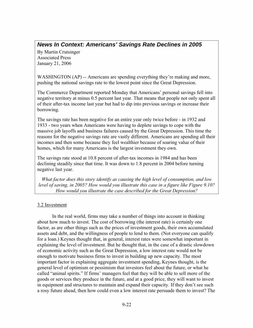
News In Context: Americans’ Savings Rate Declines in 2005 By Martin Crutsinger Associated Press January 21, 2006 WASHINGTON (AP) -- Americans are spending everything they’re making and more, pushing the national savings rate to the lowest point since the Great Depression.
The Commerce Department reported Monday that Americans’ personal savings fell into negative territory at minus 0.5 percent last year. That means that people not only spent all of their after-tax income last year but had to dip into previous savings or increase their borrowing.
The savings rate has been negative for an entire year only twice before - in 1932 and 1933 - two years when Americans were having to deplete savings to cope with the massive job layoffs and business failures caused by the Great Depression. This time the reasons for the negative savings rate are vastly different. Americans are spending all their incomes and then some because they feel wealthier because of soaring value of their homes, which for many Americans is the largest investment they own.
The savings rate stood at 10.8 percent of after-tax incomes in 1984 and has been declining steadily since that time. It was down to 1.8 percent in 2004 before turning negative last year.
What factor does this story identify as causing the high level of consumption, and low level of saving, in 2005? How would you illustrate this case in a figure like Figure 9.10?
How would you illustrate the case described for the Great Depression?
3.2 Investment In the real world, firms may take a number of things into account in thinking about how much to invest. The cost of borrowing (the interest rate) is certainly one factor, as are other things such as the prices of investment goods, their own accumulated assets and debt, and the willingness of people to lend to them. (Not everyone can qualify for a loan.) Keynes thought that, in general, interest rates were somewhat important in explaining the level of investment. But he thought that, in the case of a drastic slowdown of economic activity such as the Great Depression, a low interest rate would not be enough to motivate business firms to invest in building up new capacity. The most important factor in explaining aggregate investment spending, Keynes thought, is the general level of optimism or pessimism that investors feel about the future, or what he called “animal spirits.” If firms’ managers feel that they will be able to sell more of the goods or services they produce in the future, and at a good price, they will want to invest in equipment and structures to maintain and expand their capacity. If they don’t see such a rosy future ahead, then how could even a low interest rate persuade them to invest? The
9-23
borrowed funds will have to be repaid; the major question for the borrower is “are my prospects for success good enough to allow me to repay this investment?” The interest rate will change the amount to be repaid at the margin, but is not the major determinant of the answer to this question. Because Keynes saw investment as future-directed, rather than related to any current, observable economic variables, the “function” for intended investment in the simple Keynesian model just says that investors intend to invest whatever investors intend to invest. All of intended investment is considered “autonomous” in this model. We can denote this as:
II = __
II
where __
II is “autonomous intended investment.” Don’t worry too much about whether to put a bar over the symbol – we’ve introduced it here just to show you that it is similar in concept to the C in the consumption function. Just as C can go up or down depending on
consumer confidence, __
II can go up or down depending on investor confidence.
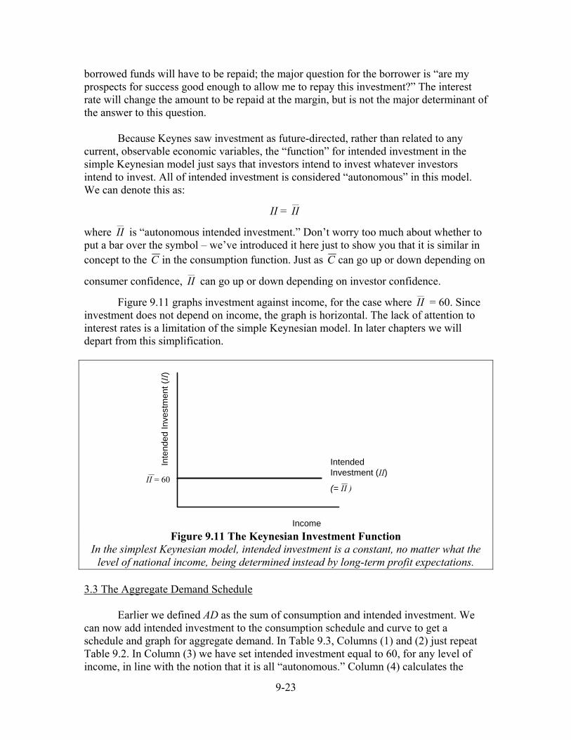
Figure 9.11 graphs investment against income, for the case where __
II = 60. Since investment does not depend on income, the graph is horizontal. The lack of attention to interest rates is a limitation of the simple Keynesian model. In later chapters we will depart from this simplification.
Income
Inte
nded
Inve
stm
ent (
II)
Intended Investment (II)
(= II )II = 60
Figure 9.11 The Keynesian Investment Function
In the simplest Keynesian model, intended investment is a constant, no matter what the level of national income, being determined instead by long-term profit expectations.
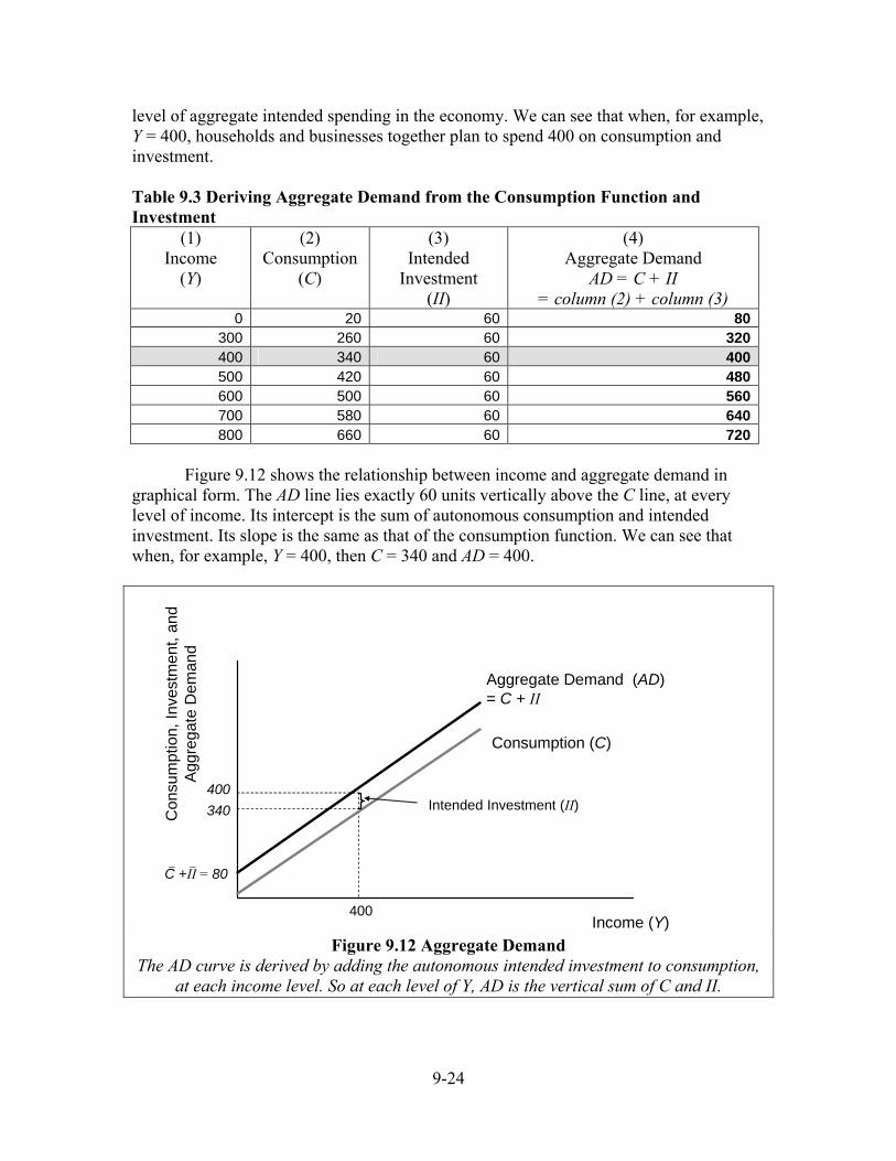
3.3 The Aggregate Demand Schedule Earlier we defined AD as the sum of consumption and intended investment. We can now add intended investment to the consumption schedule and curve to get a schedule and graph for aggregate demand. In Table 9.3, Columns (1) and (2) just repeat Table 9.2. In Column (3) we have set intended investment equal to 60, for any level of income, in line with the notion that it is all “autonomous.” Column (4) calculates the
9-24
level of aggregate intended spending in the economy. We can see that when, for example, Y = 400, households and businesses together plan to spend 400 on consumption and investment. Table 9.3 Deriving Aggregate Demand from the Consumption Function and Investment
Figure 9.12 shows the relationship between income and aggregate demand in
graphical form. The AD line lies exactly 60 units vertically above the C line, at every level of income. Its intercept is the sum of autonomous consumption and intended investment. Its slope is the same as that of the consumption function. We can see that when, for example, Y = 400, then C = 340 and AD = 400.
Consumption (C)
Income (Y)
Con
sum
ptio
n, In
vest
men
t, an
d A
ggre
gate
Dem
and
400
400
Aggregate Demand (AD) = C + II
Intended Investment (II)340
80C +II =
Figure 9.12 Aggregate Demand
The AD curve is derived by adding the autonomous intended investment to consumption, at each income level. So at each level of Y, AD is the vertical sum of C and II.
9-25
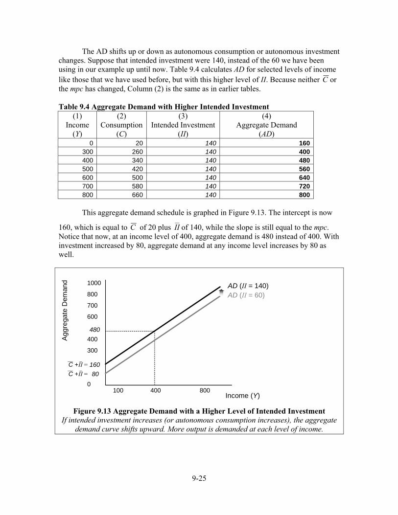
The AD shifts up or down as autonomous consumption or autonomous investment changes. Suppose that intended investment were 140, instead of the 60 we have been using in our example up until now. Table 9.4 calculates AD for selected levels of income like those that we have used before, but with this higher level of II. Because neither C or the mpc has changed, Column (2) is the same as in earlier tables. Table 9.4 Aggregate Demand with Higher Intended Investment
This aggregate demand schedule is graphed in Figure 9.13. The intercept is now
160, which is equal to C of 20 plus __
II of 140, while the slope is still equal to the mpc. Notice that now, at an income level of 400, aggregate demand is 480 instead of 400. With investment increased by 80, aggregate demand at any income level increases by 80 as well.
Income (Y)
Agg
rega
te D
eman
d
400100
1000
800
700
600
500
400
300
200
100
0
AD (II = 140)
800
480
160C +II =80C +II =
AD (II = 60)
Figure 9.13 Aggregate Demand with a Higher Level of Intended Investment
If intended investment increases (or autonomous consumption increases), the aggregate demand curve shifts upward. More output is demanded at each level of income.
9-26
Figure 9.13 could also be used to illustrate an increase in C from 20 to 100 (an
increase of 80) while intended investment remains at 60. Any combination of C and __
II that sums to 160 would yield this graph. In economic terms, any increase in consumer and investor desired spending (that is unrelated to changes in income) increases aggregate demand. 3.4 The Possibility of Unintended Investment The key to understanding the Keynesian model is understanding why and how unintended investment can occur, and how firms respond when they see it happening. Unintended investment occurs when aggregate demand is insufficient, because in this case firms will not be able to sell all the goods they produce. Recall (from Chapter 5) that a nation’s manufactured capital stock includes structures, equipment, and inventories. Many firms normally plan to keep as inventory some level of supplies they expect to use soon and products that they have not yet shipped out. Unintended inventory investment occurs when these inventories build up unexpectedly. A manufacturing firm, for example, experiences excess inventory accumulation when it can’t sell its goods as quickly as expected and the goods pile up in warehouses. Conversely, a firm that sells its goods faster than expected experiences excess inventory depletion, as the goods “fly off the shelves” and the warehouse empties out. Actual investment (I, as measured in the national accounts) is the sum of what businesses plan to invest, plus what they inadvertently end up investing if AD and Y don’t exactly match up:
I = intended investment + excess inventory accumulation or depletion
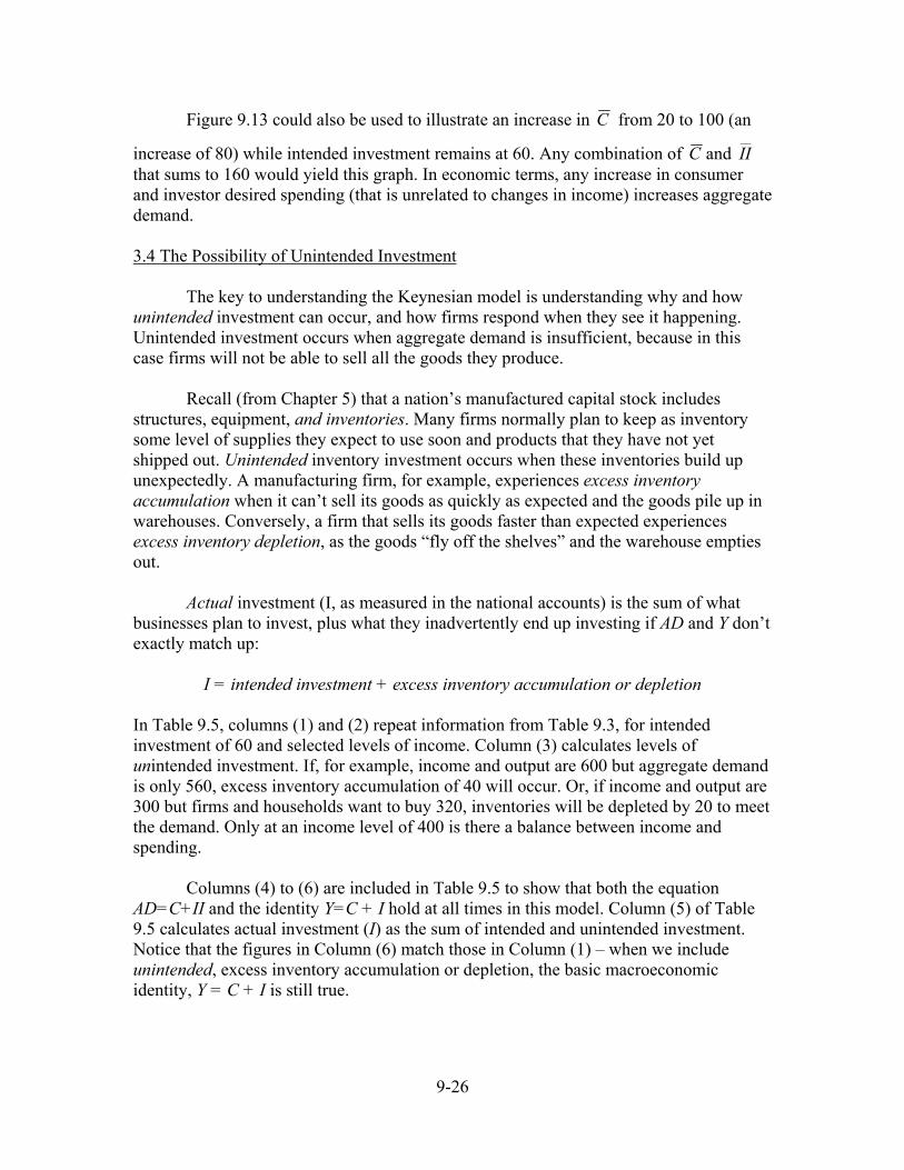
In Table 9.5, columns (1) and (2) repeat information from Table 9.3, for intended investment of 60 and selected levels of income. Column (3) calculates levels of unintended investment. If, for example, income and output are 600 but aggregate demand is only 560, excess inventory accumulation of 40 will occur. Or, if income and output are 300 but firms and households want to buy 320, inventories will be depleted by 20 to meet the demand. Only at an income level of 400 is there a balance between income and spending.
Columns (4) to (6) are included in Table 9.5 to show that both the equation AD=C+II and the identity Y=C + I hold at all times in this model. Column (5) of Table 9.5 calculates actual investment (I) as the sum of intended and unintended investment. Notice that the figures in Column (6) match those in Column (1) – when we include unintended, excess inventory accumulation or depletion, the basic macroeconomic identity, Y = C + I is still true.
9-27
Table 9.5 The Possibility of Excess Inventory Accumulation or Depletion (1)
Income (Y)
(2) Aggregate Demand
(AD)
(3) Excess Inventory Accumulation (+) or Depletion (-) = column(1)-
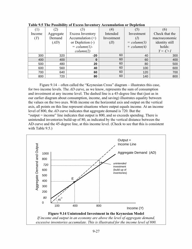
Figure 9.14 – often called the “Keynesian Cross” diagram – illustrates this case, for two income levels. The AD curve, as we know, represents the sum of consumption and investment at any income level. The dashed line is a 45-degree line that (just as in our earlier diagram about consumption, income, and saving) illustrates equality between the values on the two axes. With income on the horizontal axis and output on the vertical axis, all points on this line represent situations where output equals income. At an income level of 800, the AD curve indicates that aggregate demand is 720. But the “output = income” line indicates that output is 800, and so exceeds spending. There is unintended inventories build-up of 80, as indicated by the vertical distance between the AD curve and the 45-degree line, at this income level. (Check to see that this is consistent with Table 9.5.)
45
Income (Y)
Agg
rega
te D
eman
d an
d O
utpu
t
Output = Income Line
400100
1000
800
700
600
500
400
300
200
100
0
Aggregate Demand (AD)
800
E
unintended investment (build up of inventories)
720
80
Figure 9.14 Unintended Investment in the Keynesian Model
If income and output in an economy are above the level of aggregate demand, excessive inventories accumulate. This is illustrated for the income level of 800.
9-28
On the other hand, at an income level of 400 there is full macroeconomic equilibrium, since output, income, and spending are all at the same level. Unintended investment is zero.
At levels of income and output above 400 in Table 9.5 and Figure 9.14, business
firms’ managers are unhappy because more and more of their goods are gathering dust. For levels of income and output below 400, their inventories are getting too low for comfort. These are not equilibrium levels of income, and the economy will not stay at any of those income levels – things will change. 3.5 Movement to Equilibrium in the Keynesian Model If firms are unhappy about unsold goods, they will do something to correct the situation. If inventories are building up more than intended, they will cut back on production. Their cutbacks in production will continue until they are no longer seeing inventories build up excessively – that is, until the level of what is actually produced matches what they can sell. Reductions in Y will continue until Y = AD. This is a little more complicated than it may at first seem, though, since any reduction in output leads to reduced income, which leads to reduced consumption, so that AD is a moving target. We will look at this complication below in section 3.7, but for now we will stay with the main story.
In Figure 9.14, above, suppose that the economy were (for reasons to be explored later) initially at an income and output level of 800. From the figure and Table 9.5, we can see that this is not an equilibrium – producers are seeing excess inventory accumulation of 80 since AD is only 720. Producers will cut back on production. The equilibrium point E is obtained when aggregate output has fallen to 400 and AD has also fallen to 400.
So, what has happened here? If you look back at Table 9.2, you can see that at the initial income level of 800 there was a “leakage” into saving of 140. But firms, we have assumed, only want to spend 60 on investment. Leakages exceeded injections by 80, aggregate demand was insufficient, and inventories of 80 built up. Firms cut back on production. They continued to cut back until inventories are back where they want them.
Yet when the economy arrives at an equilibrium, the balance between saving and
investing has been restored! Why is this so? Intended investment has not changed – it has been at 60 all along. But now that income has dropped, households have less income to use for consumption and saving, and so saving has dropped from its initial level of 140 to only 60. (See Table 9.2 to check that this is the level of saving at an income level of 400.) It is changes in aggregate income, and the changes that this causes in consumption and saving, that have caused leakages and injections to become equal again! We can also see in the schedules and graphs what would happen if AD were for some reason to be above the current level of output. If output were to start out at 300, for example, desired spending of 320 (see Table 9.5) would cause produced goods to “fly off
9-29
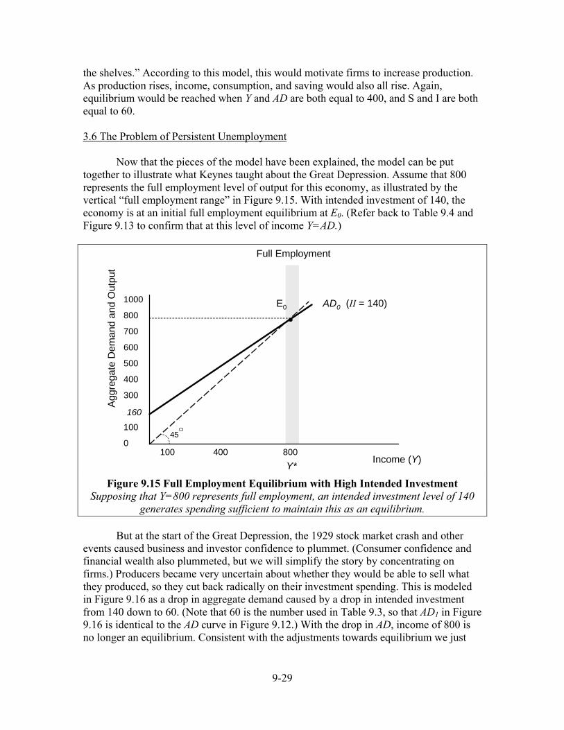
the shelves.” According to this model, this would motivate firms to increase production. As production rises, income, consumption, and saving would also all rise. Again, equilibrium would be reached when Y and AD are both equal to 400, and S and I are both equal to 60. 3.6 The Problem of Persistent Unemployment Now that the pieces of the model have been explained, the model can be put together to illustrate what Keynes taught about the Great Depression. Assume that 800 represents the full employment level of output for this economy, as illustrated by the vertical “full employment range” in Figure 9.15. With intended investment of 140, the economy is at an initial full employment equilibrium at E0. (Refer back to Table 9.4 and Figure 9.13 to confirm that at this level of income Y=AD.)
45
Income (Y)
Agg
rega
te D
eman
d an
d O
utpu
t
400100
1000
800
700
600
500
400
300
200
100
0
AD0 (II = 140)
800
160
E0
Full Employment
Y*
Figure 9.15 Full Employment Equilibrium with High Intended Investment Supposing that Y=800 represents full employment, an intended investment level of 140
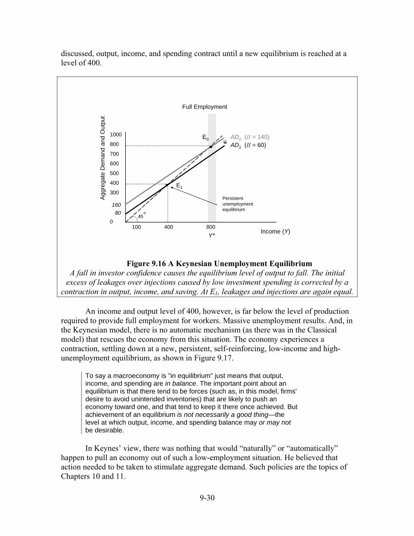
generates spending sufficient to maintain this as an equilibrium. But at the start of the Great Depression, the 1929 stock market crash and other events caused business and investor confidence to plummet. (Consumer confidence and financial wealth also plummeted, but we will simplify the story by concentrating on firms.) Producers became very uncertain about whether they would be able to sell what they produced, so they cut back radically on their investment spending. This is modeled in Figure 9.16 as a drop in aggregate demand caused by a drop in intended investment from 140 down to 60. (Note that 60 is the number used in Table 9.3, so that AD1 in Figure 9.16 is identical to the AD curve in Figure 9.12.) With the drop in AD, income of 800 is no longer an equilibrium. Consistent with the adjustments towards equilibrium we just
9-30
discussed, output, income, and spending contract until a new equilibrium is reached at a level of 400.
45
Income (Y)
Agg
rega
te D
eman
d an
d O
utpu
t
400100
1000
800
700
600
500
400
300
200
100
0
AD0 (II = 140)
800
E1
16080
E0
Full Employment
AD1 (II = 60)
Persistent unemployment equilibrium
Y*
Figure 9.16 A Keynesian Unemployment Equilibrium
A fall in investor confidence causes the equilibrium level of output to fall. The initial excess of leakages over injections caused by low investment spending is corrected by a
contraction in output, income, and saving. At E1, leakages and injections are again equal. An income and output level of 400, however, is far below the level of production
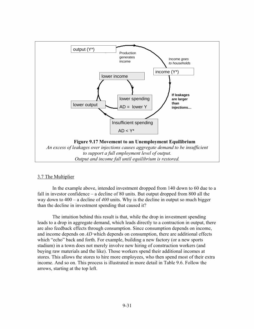
required to provide full employment for workers. Massive unemployment results. And, in the Keynesian model, there is no automatic mechanism (as there was in the Classical model) that rescues the economy from this situation. The economy experiences a contraction, settling down at a new, persistent, self-reinforcing, low-income and high-unemployment equilibrium, as shown in Figure 9.17.
To say a macroeconomy is "in equilibrium" just means that output, income, and spending are in balance. The important point about an equilibrium is that there tend to be forces (such as, in this model, firms' desire to avoid unintended inventories) that are likely to push an economy toward one, and that tend to keep it there once achieved. But achievement of an equilibrium is not necessarily a good thing—the level at which output, income, and spending balance may or may not be desirable. In Keynes’ view, there was nothing that would “naturally” or “automatically”
happen to pull an economy out of such a low-employment situation. He believed that action needed to be taken to stimulate aggregate demand. Such policies are the topics of Chapters 10 and 11.
9-31
output (Y*)
income (Y*)
Insufficient spending
AD < Y*
Production generates income
Income goes to households
If leakages are larger than injections…
lower income
lower spending
AD = lower Ylower output
Figure 9.17 Movement to an Unemployment Equilibrium
An excess of leakages over injections causes aggregate demand to be insufficient to support a full employment level of output.
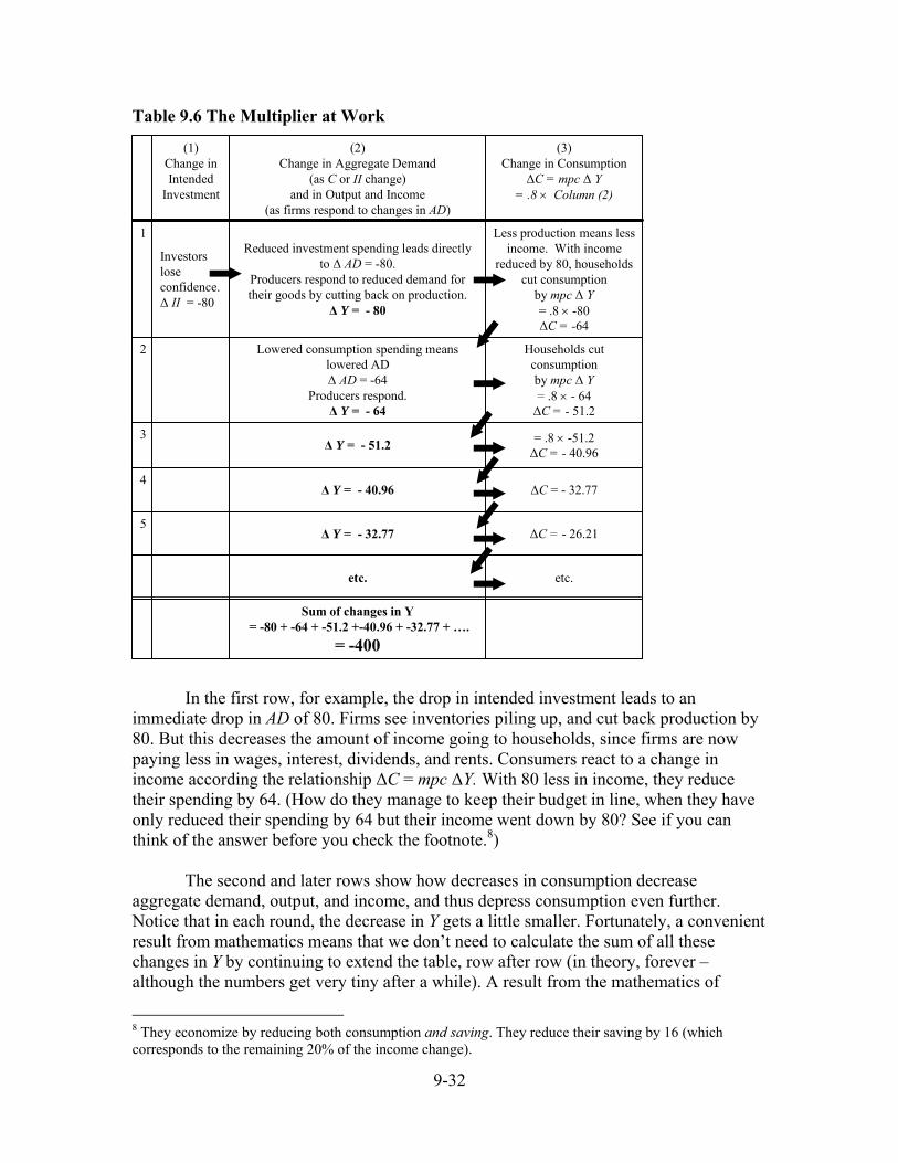
Output and income fall until equilibrium is restored. 3.7 The Multiplier In the example above, intended investment dropped from 140 down to 60 due to a fall in investor confidence – a decline of 80 units. But output dropped from 800 all the way down to 400 – a decline of 400 units. Why is the decline in output so much bigger than the decline in investment spending that caused it? The intuition behind this result is that, while the drop in investment spending leads to a drop in aggregate demand, which leads directly to a contraction in output, there are also feedback effects through consumption. Since consumption depends on income, and income depends on AD which depends on consumption, there are additional effects which “echo” back and forth. For example, building a new factory (or a new sports stadium) in a town does not merely involve new hiring of construction workers (and buying raw materials and the like). Those workers spend their additional incomes at stores. This allows the stores to hire more employees, who then spend most of their extra income. And so on. This process is illustrated in more detail in Table 9.6. Follow the arrows, starting at the top left.
9-32
Table 9.6 The Multiplier at Work
Sum of changes in Y= -80 + -64 + -51.2 +-40.96 + -32.77 + ….
Lowered consumption spending means lowered AD∆ AD = -64
Producers respond.∆ Y = - 64
2
Less production means less income. With income
reduced by 80, households cut consumption
by mpc ∆ Y= .8 × -80∆C = -64
Reduced investment spending leads directly to ∆ AD = -80.
Producers respond to reduced demand for their goods by cutting back on production.
∆ Y = - 80
Investors lose confidence.∆ II = -80
1
(3)Change in Consumption
∆C = mpc ∆ Y= .8 × Column (2)
(2)Change in Aggregate Demand
(as C or II change)and in Output and Income
(as firms respond to changes in AD)
(1)Change in Intended
Investment
In the first row, for example, the drop in intended investment leads to an immediate drop in AD of 80. Firms see inventories piling up, and cut back production by 80. But this decreases the amount of income going to households, since firms are now paying less in wages, interest, dividends, and rents. Consumers react to a change in income according the relationship ∆C = mpc ∆Y. With 80 less in income, they reduce their spending by 64. (How do they manage to keep their budget in line, when they have only reduced their spending by 64 but their income went down by 80? See if you can think of the answer before you check the footnote.8) The second and later rows show how decreases in consumption decrease aggregate demand, output, and income, and thus depress consumption even further. Notice that in each round, the decrease in Y gets a little smaller. Fortunately, a convenient result from mathematics means that we don’t need to calculate the sum of all these changes in Y by continuing to extend the table, row after row (in theory, forever – although the numbers get very tiny after a while). A result from the mathematics of
8 They economize by reducing both consumption and saving. They reduce their saving by 16 (which corresponds to the remaining 20% of the income change).
9-33
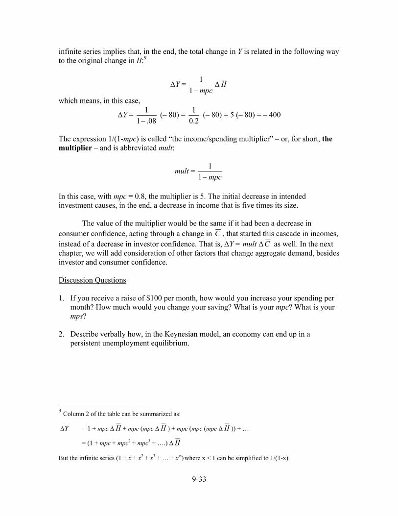
infinite series implies that, in the end, the total change in Y is related in the following way to the original change in II:9
∆Y = mpc−11 ∆
__
II
which means, in this case,
∆Y = 08.1
1−
(– 80) = 2.0
1 (– 80) = 5 (– 80) = – 400
The expression 1/(1-mpc) is called “the income/spending multiplier” – or, for short, the multiplier – and is abbreviated mult:
mult = mpc−11
In this case, with mpc = 0.8, the multiplier is 5. The initial decrease in intended investment causes, in the end, a decrease in income that is five times its size. The value of the multiplier would be the same if it had been a decrease in consumer confidence, acting through a change in C , that started this cascade in incomes, instead of a decrease in investor confidence. That is, ∆Y = mult ∆C as well. In the next chapter, we will add consideration of other factors that change aggregate demand, besides investor and consumer confidence. Discussion Questions 1. If you receive a raise of $100 per month, how would you increase your spending per
month? How much would you change your saving? What is your mpc? What is your mps?
2. Describe verbally how, in the Keynesian model, an economy can end up in a
persistent unemployment equilibrium.
9 Column 2 of the table can be summarized as:
∆Y = 1 + mpc ∆__
II + mpc (mpc ∆__
II ) + mpc (mpc (mpc ∆__
II )) + …
= (1 + mpc + mpc2 + mpc3 + ….) ∆__
II
But the infinite series (1 + x + x2 + x3 + … + x∞) where x < 1 can be simplified to 1/(1-x).
9-34
4. Concluding Thoughts In the Classical economic theory, an economy should never go into a slump – or at least it should not stay in one very long. Any deficiency in aggregate demand would be quickly counteracted by smooth adjustments in the market for loanable funds. Keynes, on the other hand, theorized that deficiencies in aggregate demand, due to drops in investor (or consumer) confidence could explain the long-term, deep slumps many countries experienced during the Great Depression (as well as some of the other economic depressions that various economies have experienced over history). Any excess of “leakages” over “injections” into the aggregate demand stream would, he theorized, lead to progressive rounds of declines in consumption and income, until saving are so low that a new, lower-output-level equilibrium is established. In the next chapter, we will explore how the U.S. economy did, in fact, get out of the Great Depression.
But take a moment to consider the implications of this model as it relates to contemporary controversies over consumerism and the environment. In the Keynesian model it does, indeed, appear that keeping consumption and spending at high levels is necessary to keep the economy humming. The idea that cutting back on consumption spending would be “bad for the economy” is based on the Keynesian notion that reductions in aggregate spending lead to recessions or depressions, and that these could potentially be deep and persistent. This inference is, however, based on the idea that a cut in wasteful spending is the same thing as a cut in aggregate spending. We will revisit this assumption in Chapter 12 to see if it really is the case that what is good for the environment (and for future generations) has to be “bad for the economy.” Discussion Questions 1. Which theory – Classical or Keynesian – seems to you more realistic in describing
today’s economy? 2. Have you ever read articles or editorials that claim that high consumption is essential
for a healthy economy? Does the Keynesian model seem to confirm or challenge this idea? What are some arguments for the opposite point of view?
Review Questions 1. During a business cycle recession, which of the following typically rises: the level of
output, the unemployment rate, and/or the inflation rate?
2. During the 1930s, how did economists' opinions about the Great Depression differ?
3. In the model laid out in this chapter, who receives income? Who spends? Who saves?
4. What is the definition of Aggregate Demand? How does it differ from measured GDP?
9-35
5. What conditions describe equilibrium in a macroeconomy?
6. Saving is described as a “leakage” from the circular flow. How is it a leakage? How is it that an increase in saving (if not balanced by an increase in intended investment) might cause a shrinkage of the output-income-spending flow?
7. Describe the Classical market for loanable funds. Who are the actors, and what do they each do?
8. Describe how the problem of leakages is solved in the Classical model.
9. How did Keynes model consumption behavior? Draw and label a graph.
10. List five factors, aside from the level of income, that may affect the level of consumption in a macroeconomy.
11. Why isn't the interest rate included in the Keynesian consumption function?
12. What did Keynes' think was the most important factor in determining investment behavior?
13. What determines Aggregate Demand in the Keynesian model? Draw and label a graph.
14. Do firms always end up investing the amount they intend? Why or why not?
15. Draw a "Keynesian Cross" diagram, carefully labeling the curves and the equilibrium point.
16. Describe how adjustment to equilibrium occurs in the Keynesian model.
17. Does a macroeconomy being "in equilibrium" always mean it is in a good state? Why or why not?
18. What is "the income/spending multiplier"? Explain why a drop in autonomous intended investment, or in autonomous consumption, leads to a much larger drop in equilibrium income.
Exercises 1. Carefully draw and label a supply and demand diagram for the Classical loanable funds market. Assuming that the market starts and ends in equilibrium, indicate what happens if there is a sudden drop in households' desire to consume.
a. Which curve shifts and in what direction?
b. What happens to the equilibrium amount of loanable funds borrowed and lent? (You do not need to put numbers on the graph—just point out the direction of the change.)
c. What happens to the equilibrium interest rate?
d. What happens to the equilibrium amount of investment?
9-36
2. Suppose you see a toy store increasing its inventories in early December, right before the Christmas/Chanukah/Kwanzaa season. Is this a case of excess inventory accumulation? Why or why not? 3. Suppose that the relation between consumption and income is C = 90 + 0.75 Y.
a. For each additional dollar that households receive, how much do they save? How much do they spend? b. What is the level of consumption when income is equal to 0? 360? 500? 600? (You may want to make a table similar to Table 9.2 in the text.) c. What is the level of saving when income is equal to 0? 360? 500? 600? d. As income rises from 500 to 600, by how much does consumption rise? What formula would you use to derive the mpc from your answer to this question, if you did not know the mpc already? e. Graph this consumption function, along with a 45-degree "consumption=income" line. Label the slope and intercept, and show how the level of savings when income is equal to 600 can be found on this graph.
4. Draw a Keynesian Cross graph and assume that the macroeconomy starts and ends in equilibrium. Label the initial aggregate demand line AD0. Then show what happens in the diagram when a rise in consumer wealth raises C (autonomous consumption) in your diagram. (This event might happen if the stock market or the housing market enjoys large price increases. You do not need to put numbers on the graph—just point out the direction of the change.)
a. How does the AD line shift? Label the new line AD1.
b. What is the initial effect of this change on inventories? How will firms change production in response to this change in inventories?
c. What happens to the equilibrium level of production, income, and spending? Does each rise, fall, or stay the same?
5. What happens in the Keynesian model if households decide to be "thriftier"—that is, spend less and save more? Do the following several-step exercise to find out.
a. Suppose the economy starts out in a situation we already developed in the text: C = 20 + .8 Y and II = 60. (See Table 9.3) Carefully graph the resulting AD curve, labeling the levels of aggregate demand that result when income is equal to 0, 300, 400, and 500. Label the curve AD0, add the 45-degree line, and label the equilibrium point E0.
b. What is the equilibrium level of income, in this initial case? What is the equilibrium level of saving?
c. Now suppose that people decide they want to save more of their income, and spend less of it. In fact, their new level of autonomous consumption is zero, so the new consumption function is just C = .8 Y . Calculate the levels of consumption and aggregate demand that would result from incomes of 0, 300, 400, and 500. (You might
9-37
want to set up a table similar to Table 9.3, but using this new equation for consumption. Intended investment is still 60).
d. If income stayed at the equilibrium level determined in part (b) of this question, would people now be saving more? How much more? Show your work.
e. Add the AD curve that arises from your calculations in part (c) on the graph you drew earlier. Label this curve AD1 and the new equilibrium point E1.
f. What is the new equilibrium level of income? What is the new equilibrium level of saving? Compare your answers to your answers to part (b).
g. Explain why this phenomenon arising from the Keynesian model is called "the paradox of thrift." Can you explain why this "paradox" arises?
6. Suppose that the behavior of households and firms in an economy is determined by the following equations:
C = 90 + 0.75 Y
II = 35
a. Show in a table what the levels of C and AD would be at income levels of 0, 500, and 600.
b. If, for some reason, income were equal to 600, would there be unintended inventory investment? If so, would inventories be excessive or depleted, and by how much?
c. If, for some reason, income were equal to 500, would there be unintended inventory investment? If so, would inventories be excessive or depleted, and by how much?
d. What is the equilibrium level of income and output?
e. What is the income/spending multiplier equal to, in this model?
f. If intended investment were to rise by 25, by how much would equilibrium income increase? Use the income/spending multiplier.
7. (Appendix) Suppose that the behavior of households and firms in an economy is determined by the following equations:
C = 50 + 0.9 Y
II = 50
Answer the following questions, using algebraic manipulations only.
a. What is the equation for the AD curve?
b. What is the level of equilibrium income?
c. If intended investment increases by 10 units to 60 units, by how much will equilibrium income rise?
9-38
8. Match each concept in Column A with a definition or example in Column B. Column A Column B
a. mult ∆__
II b. an injection c. An assumption evident in the
equation AD = C + II d. Okun's "law" e. a Classical assumption about
saving f. unintended investment g. the turning point from a business
cycle expansion to contraction h. mpc i. the intercept of the AD curve j. a Keynesian assumption about
saving
i. peak ii. an inverse relationship
between unemployment and rapid GDP growth
iii. households save more when income rises
iv. I – II v. the proportion of an
additional dollar that households spend on consumption
vi. C + __
II vii. the amount that
equilibrium GDP rises when autonomous investment rises
viii. households save more when the interest rate rises
ix. no government sector x. intended investment
9-39
Appendix: An Algebraic Approach to the Multiplier The formula for the multiplier in the simplest Keynesian model can also be derived using tools of basic algebra, starting with rearranging the equation for AD:
AD = C + II we can substitute in for consumption, C = C + mpc Y, and use the fact that in this model all investment is autonomous, to get
AD = (C + mpc Y) + __
II
= (C +__
II ) + mpc Y
The last rearrangement shows that the AD curve has an intercept equal to the sum of the autonomous terms and a slope equal to the marginal propensity to consume. Changes in either of the variable in parentheses, by changing the intercept, shift the curve up or down in a parallel manner.
By substituting this into the equation for the equilibrium condition, Y = AD, we can derive an expression for equilibrium income in terms of all the other variables in the model:
Y = (C +__
II ) + mpc Y
Y – mpc Y = C + __
II
(1- mpc)Y = C + __
II
Y = mpc−11 (C +
__
II )
If autonomous consumption, intended investment, or government spending change, these each increase equilibrium income by mult=1/(1-mpc) times.
To see this explicitly, consider the changes that would come about in Y if there is
a change in __
II from 0
__II to a new level, 1
__II , if autonomous consumption (and the mpc)
stays the same. We can solve for the change in Y by subtracting the old equation from the new one:
Y1 = mpc−11 (C + 1
__II )
– Y0 = mpc−11 (C + 0
__II )
Y1 – Y0 = mpc−11 (C –C + 1
__II – 0
__II )
9-40
But C (and the mpc) is unchanged, so the first subtraction in parentheses comes out to be zero. We are left with:
Y1 – Y0 = mpc−11 ( 1
__II – 0
__II )
or
∆Y =mult ∆__
II where mult=1/(1-mpc). Similar analysis of ∆C (holding intended investment constant) would show that the multiplier for that change is also mult.