Chapter 9 Basic Signal Processing - cs.princeton.edu 9 Basic Signal Processing ... Digital Signal...

Chapter 9

Basic Signal Processing

Motivation

Many aspects of computer graphics and computer imagery differ from aspects ofconventional graphics and imagery because computer representations are digital anddiscrete, whereas natural representations are continuous. In a previous lecture wediscussed the implications of quantizing continuous or high precision intensity val-ues to discrete or lower precision values. In this sequence of lectures we discuss theimplications of sampling a continuous image at a discrete set of locations (usuallya regular lattice). The implications of the sampling process are quite subtle, and tounderstand them fully requires a basic understanding of signal processing. Thesenotes are meant to serve as a concise summary of signal processing for computergraphics.

Reconstruction

Recall that a framebuffer holds a 2D array of numbers representing intensities. Thedisplay creates a continuous light image from these discrete digital values. We saythat the discrete image is reconstructed to form a continuous image.

Although it is often convenient to think of each 2D pixel as a little square thatabuts its neighbors to fill the image plane, this view of reconstruction is not verygeneral. Instead it is better to think of each pixel as a point sample. Imagine animage as a surface whose height at a point is equal to the intensity of the image atthat point. A single sample is then a “spike;” the spike is located at the position ofthe sample and its height is equal to the intensity associated with that sample. Thediscrete image is a set of spikes, and the continuous image is a smooth surface fittingthe spikes as shown in Figure 9.1. One obvious method of forming the continuoussurface is to interpolate between the samples.

1

2 CHAPTER 9. BASIC SIGNAL PROCESSING

Figure 9.1: A continuous image reconstructed from a discrete image represented asa set of samples. In this figure, the image is drawn as a surface whose height is equalto the intensity.

Sampling

We can make a digital image from an analog image by taking samples. Most simply,each sample records the value of the image intensity at a point.

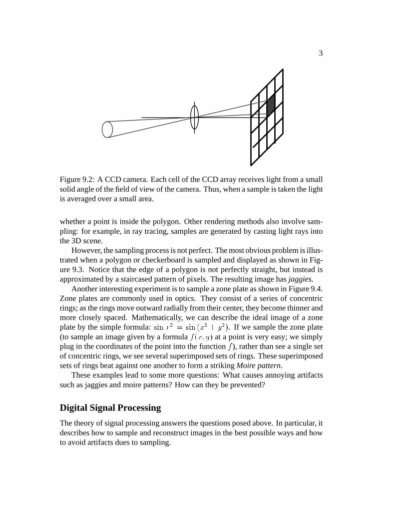
Consider a CCD camera. A CCD camera records image values by turning lightenergy into electrical energy. The light sensitive area consist of an array of smallcells; each cell produces a single value, and hence, samples the image. Notice thateach sample is the result of all the light falling on a single cell, and corresponds toan integral of all the light within a small solid angle (see Figure 9.2). Your eye issimilar, each sample results from the action of a single photoreceptor. However, justlike CCD cells, photoreceptor cells are packed together in your retina and integrateover a small area. Although it may seem like the fact that an individual cell of aCCD camera, or of your retina, samples over an area is less than ideal, the fact thatintensities are averaged in this way will turn out to be an important feature of thesampling process.

A vidicon camera samples an image in slightly different way than your eye ora CCD camera. Recall that television signal is produced by a raster scan process inwhich the beams moves continuously from left to right, but discretely from top tobottom. Therefore, in television, the image is continuous in the horizontal direction.and sampled in the vertical direction.

The above discussion of reconstruction and sampling leads to an interesting ques-tion: Is it possible to sample an image and then reconstruct it without any distortion?

Jaggies, Aliasing

Similarly, we can create digital images directly from geometric representations suchas lines and polygons. For example, we can convert a polygon to samples by testing

3

Figure 9.2: A CCD camera. Each cell of the CCD array receives light from a smallsolid angle of the field of view of the camera. Thus, when a sample is taken the lightis averaged over a small area.

whether a point is inside the polygon. Other rendering methods also involve sam-pling: for example, in ray tracing, samples are generated by casting light rays intothe 3D scene.

However, the sampling process is not perfect. The most obvious problem is illus-trated when a polygon or checkerboard is sampled and displayed as shown in Fig-ure 9.3. Notice that the edge of a polygon is not perfectly straight, but instead isapproximated by a staircased pattern of pixels. The resulting image has jaggies.

Another interesting experiment is to sample a zone plate as shown in Figure 9.4.Zone plates are commonly used in optics. They consist of a series of concentricrings; as the rings move outward radially from their center, they become thinner andmore closely spaced. Mathematically, we can describe the ideal image of a zoneplate by the simple formula: �� . If we sample the zone plate(to sample an image given by a formula � �� at a point is very easy; we simplyplug in the coordinates of the point into the function � ), rather than see a single setof concentric rings, we see several superimposed sets of rings. These superimposedsets of rings beat against one another to form a striking Moire pattern.

These examples lead to some more questions: What causes annoying artifactssuch as jaggies and moire patterns? How can they be prevented?

Digital Signal Processing

The theory of signal processing answers the questions posed above. In particular, itdescribes how to sample and reconstruct images in the best possible ways and howto avoid artifacts dues to sampling.


Figure 9.3: A ray traced image of a 3D scene. The image is shown at full resolutionon the left and magnified on the right. Note the jagged edges along the edges of thecheckered pattern.

Signal processing is very useful tool in computer graphics and image processing.There are many other applications of signal processing ideas, for example:

1. Images can be filtered to improve their appearance. Sometimes an image hasbeen blurred while it was acquired (for example, if the camera was moving)and it can be sharpened to look less blurry.

2. Multiple signals (or images) can be cleverly combined into a single signal,so that the different components can later be extracted from the single signal.This is important in television, where different color images are combined toform a single signal which is broadcast.

Frequency Domain vs. Spatial Domain

The key to understanding signal processing is to learn to think in the frequency do-main.

Let’s begin with a mathematical fact: Any periodic function (except various mon-strosities that will not concern us) can always be written as a sum of sine and cosinewaves.

5

Figure 9.4: Sampling the equation �� . Rather than a single set of ringscentered at the origin, notice there are several sets of superimposed rings beatingagainst each other to form a pronounced Moire pattern.


A periodic function is a function defined in an interval that repeats itself out-side the interval. The sine function— ��!� —is perhaps the simplest periodic func-tion and has an interval equal to "$# . It is easy to see that the sine function is periodicsince ��%� "$# �&'��(� . Sines can have other frequencies, for example, the sinefunction �� ")#�� repeats itself � times in the interval from * to "$# . � is the fre-quency of the sine function and is measured in cycles per second or Hertz.

If we could represent a periodic function with a sum of sine waves each of whoseperiods were harmonics of the period of the original function, then the resulting sumwill also be periodic (since all the sines are periodic). The above mathematical factsays that such a sum can always be found. The reason we can represent all periodicfunctions is that we are free to choose the coefficients of each sine of a differentfrequency, and that we can use an infinite number of higher and higher frequencysine waves.

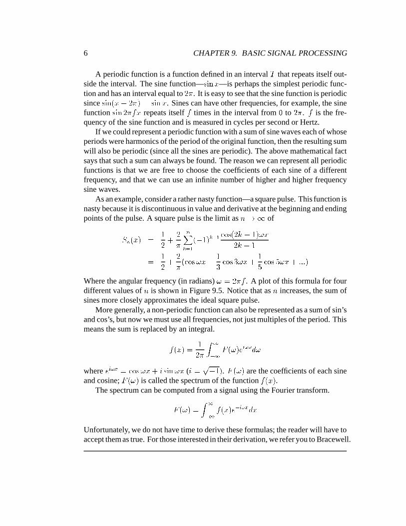
As an example, consider a rather nasty function—a square pulse. This function isnasty because it is discontinuous in value and derivative at the beginning and endingpoints of the pulse. A square pulse is the limit as +-, . of/�0 �1�2�3 4" � "#

05687:9 �8; 4 � 6�<�9)=�> �� ")? ; 4 �A@&�")? ; 4 4" � "# � =B> �C@&�D;E4F =�> � F @&�G�E4H =�> � H @I�J�LK�K�KM�Where the angular frequency (in radians) @L ")#�� . A plot of this formula for fourdifferent values of + is shown in Figure 9.5. Notice that as + increases, the sum ofsines more closely approximates the ideal square pulse.

More generally, a non-periodic function can also be represented as a sum of sin’sand cos’s, but now we must use all frequencies, not just multiples of the period. Thismeans the sum is replaced by an integral.

� �1�N�O 4"$# PRQ< QTS �U@V�XW�Y[Z]\_^]@where W Y`Z�\ =�> ��@&�%�bac��@&� ( aIed ; 4 � . S �f@V� are the coefficients of each sineand cosine; S �f@V� is called the spectrum of the function � �1�2� .

The spectrum can be computed from a signal using the Fourier transform.

S �U@V�O PRQ< Q � �1�N�XW < Y`Z�\�^c�Unfortunately, we do not have time to derive these formulas; the reader will have toaccept them as true. For those interested in their derivation, we refer you to Bracewell.

7

/ 9 / �

/ � / 9hgFigure 9.5: Four approximations to a square pulse. Notice that each approximationinvolves higher frequency terms and the resulting sum more closely approximatesthe pulse. As more and more high frequencies are added, the sum converges exactlyto the square pulse. Note also the oscillation at the edge of the pulse; this is oftenreferred to as the Gibbs phenomena.


To illustrate the mathematics of the Fourier transform, let us calculate the Fouriertransform of a square pulse. A square pulse is described mathematically as

�8icj�k]lXmc��2�Oon 4 p � prq 9�* p � prs 9�

The Fourier transform of this function is straightforward to compute.PGQ< Q �XiCjtk]l8mr��2��W < Y`Z�\u^c� Pwvx< vx W < Y`Z�\y^c� W < Y[Z]\;(aU@ p vx< vx W Y vx Z ;zW < Y vx Z" a 9� @ �� 9� @9� @ �� = �Here we introduce the �� = function defined to be�� = �{ �� # �# �

Note that �� # � equals zero for all integer values of � , except � equals zero. At zero,the situation is more complicated: both the numerator and the denominator are zero.However, careful analysis shows that �� = * 4 .

Thus, �� = � + �Oon 4 + ** +w| *A plot of the sinc function is shown below. Notice that the amplitude of the oscilla-tion decreases as � moves from the origin.

9

It is important to build up your intuition about functions and their spectra. Fig-ure 9.6 shows some example functions and their Fourier transforms.

The Fourier transform of =�> �!@&� is two spikes, one at ;V@ and the other at �V@ .This should be intuitively true because the Fourier transform of a function is an ex-pansion of the function in terms of sines and cosines. But, expanding either a singlesine or a single cosine in terms of sines and cosines yields the original sine or cosine.Note, however, that the Fourier transform of a cosine is two positive spikes, whereasFourier transform of a sine is one negative and one positive spike. This follows fromthe property that the cosine is an even function ( =�> �2;V@O}� =B> �C@O} ) whereas the sineis an odd function ( �� ;~@O}Oe;��@O} ).

The Fourier transform of a constant function is a single spike at the origin. Onceagain this should be intuitively true. A constant function does not vary in time orspace, and hence, does not contain sines or cosines with non-zero frequencies.

Comparing the formula for the Fourier transform with the formula for the inverseFourier transform, we see that they differ only in the sign of the argument to theexponential. This implies that Fourier transform and the inverse Fourier transformare qualitatively the same. Thus, if we know the transform from the space domainto the frequency domain, we also know the transform from the frequency domain tothe space domain. Thus, the Fourier transform of a single spike at the origin consistsof sines and cosines of all frequencies equally weighted.

In the above discussion we have used the term spike several times without prop-erly defining it. A delta function has the property that it is zero everywhere exceptat the origin. � ��2�� * � | *The value of the delta function is not really defined, but its integral is. That is,PRQ� � ��2��^c� 4


�

�

�

�

�

Space Frequency

Figure 9.6: Fourier transform pairs. From top to bottom: =�> ��@&� , ��@&� ,� �1�N� ,��tk]�u��2� , and W < \ x .

11

Figure 9.7: An image and its Fourier transform

One imagines a delta function to be a square pulse of unit area in the limit as the baseof the pulse becomes narrower and narrower and goes towards zero.

The example Fourier transform pairs also illustrate two other functions. TheFourier transform of a sequence of spikes consist of a sequence of spikes (a sequenceof spikes is sometimes referred to as the shah function). This will be very usefulwhen discussing sampling.

It also turns out that the Fourier transform of a Gaussian is equal to a Gaussian.The spectrum of a function tells the relative amounts of high and low frequencies

in the function. Rapid changes imply high frequencies, gradual changes imply lowfrequencies. The zero frequency component, or dc term, is the average value of thefunction.

The above ideas apply equally to images. Figure 9.7 shows the ray traced pictureand its Fourier transform. In an image, high frequency components contribute tofine detail, sharp edges, etc. and low frequency components represent large objectsor regions.

Another important concept is that of a bandlimited function. A function is ban-dlimited if its spectrum has no frequencies above some maximum frequency. Saidanother way, the spectra of a bandlimited function occupies a finite interval of fre-quencies, not the entire frequency range.

To summarize: the key point of this section is that a function � can be easilyconverted from the space domain (that is, a function of � ) to the frequency domain


×

=

×

×

=

=

Figure 9.8: Perfect low-pass (top), high-pass (middle), and band-pass (bottom) fil-ters.

(that is, a function, albeit a different function, of @ ), and vice versa. Thus, a func-tion can be interpreted in either of two domains: the space or the frequency domain.The Fourier transform and the inverse Fourier transform can be used to interconvertbetween the two domains. Some properties and operations on functions are easierto see in the space domain, others are easier to see in the frequency domain.

Convolution and Filtering

The spectrum of a function can be modified to attenuate or enhance different fre-quencies. Modifying a signal or an image in this way is called filtering. Mathemat-ically, the properties of filters are easiest to describe in the frequency domain.� �U@!�I S �U@!�V�-��U@V�Here,

�is the spectrum of the filtered function, S is the spectrum of the original

function, and � is the spectrum of the filter. The symbol � indicates simple multi-plication. Each frequency component of the input function is multiplied by the cor-responding frequency component of the filter function to compute the value of theoutput function at that frequency component.

The effects of filters are shown in Figure 9.8. Filters are characterized by howthey change different frequency components. A low-pass filter attenuates high fre-quencies relative to low frequencies; a high-pass filter attenuates low frequenciesrelative to high frequencies; a band-pass filter preserves a range of frequencies rela-tive to those outside that range. A perfect low-pass filter leaves all frequencies below

13

Figure 9.9: Application of a low-pass filter to an image. Notice that the resulting im-age on the right is blurry. This is because the filter removes all the high frequencieswhich represent fine detail.

it cut-off frequency and removes all frequencies above the cut-off frequency. Thus,in the frequency domain, a low-pass filter is a square pulse (see Figure 9.8). Simi-larly, a perfect high-pass filter completely removes all frequencies below the cut-offfrequency, and a perfect band-pass filter removes all frequencies outside its band.

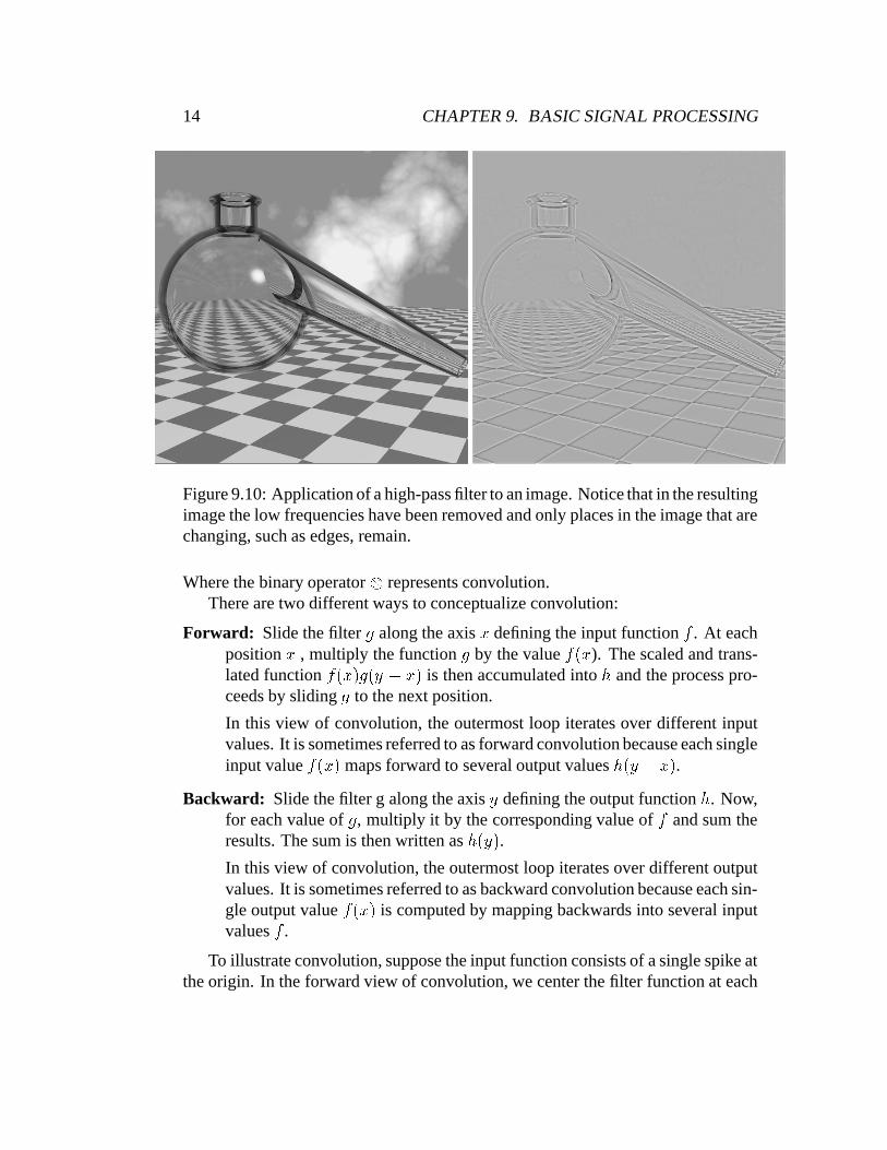
When an image is filtered, the effect is very noticeable. Removing high frequen-cies leaves a blurry image (see Figure 9.9). Removing low frequencies enhancesthe high frequencies and creates a sharper image containing mostly edges and otherrapidly changing textures (see Figure 9.10). The cutoff frequency for the high passand the low pass filter is the same in the examples shown in Figure 9.9 and Fig-ure 9.10. Since the sum of the low and high pass filters is 1, the sum of the filteredpictures must equal the original picture. Therefore, if the pictures in the right handcolumn are added together, the original picture in the left hand column is returned.

The properties of filters are easiest to see in the frequency domain. However, itis important to be able to apply filters in either the frequency domain or the spacedomain. In the frequency domain, filtering is achieved by simply multplying spec-tra, value by value. In the space domain, filtering is achieved by a more complicatedoperation called convolution.� ��O �R�� PRQ< Q � �1�2� � �� ;w�2��^c�


Figure 9.10: Application of a high-pass filter to an image. Notice that in the resultingimage the low frequencies have been removed and only places in the image that arechanging, such as edges, remain.

Where the binary operator � represents convolution.There are two different ways to conceptualize convolution:

Forward: Slide the filter � along the axis � defining the input function � . At eachposition � , multiply the function � by the value � �� ). The scaled and trans-lated function � ��2� � �1�J;b�2� is then accumulated into

�and the process pro-

ceeds by sliding � to the next position.

In this view of convolution, the outermost loop iterates over different inputvalues. It is sometimes referred to as forward convolution because each singleinput value � ��2� maps forward to several output values

� ��w�2� .Backward: Slide the filter g along the axis � defining the output function

�. Now,

for each value of � , multiply it by the corresponding value of � and sum theresults. The sum is then written as

� �� .In this view of convolution, the outermost loop iterates over different outputvalues. It is sometimes referred to as backward convolution because each sin-gle output value � ��2� is computed by mapping backwards into several inputvalues � .

To illustrate convolution, suppose the input function consists of a single spike atthe origin. In the forward view of convolution, we center the filter function at each

15

Figure 9.11: Convolution of two square pulses

point along the input function and multiply the filter everywhere by the value of thefunction. If the input is a single spike at the origin, then the input function is zeroeverywhere except at zero. Thus, the filter is multiplied by zero everywhere exceptat the origin where it is multipled by one. Therefore, the result of convolving thefilter by a delta function is the filter itself. Mathematically, this follows immediatelyfrom the definition of the delta function.PRQ< Q � ��2� � �� ;w�N��^c� � ��

Many physical processes may be described as filters. If such a process is drivena delta function, or impulse, the output will the be characteristic filtering functionof the system. For this reason, filters are sometimes referred to as impulse responsefunctions.

Convolution is a very important idea so let us consider another example—theconvolution of two square pulses as shown in Figure 9.11. The figure shows theconvolution as a backward mapping. One square pulse, the one corresponding tothe input signal, is shown stationary and centered at the origin. The other squarepulse, representing the filter, moves along the output axis from left to right. Each


�Square Sinc

�Triangle = Square � Square � �� = �

�Cubic � �� =��

Space Frequency

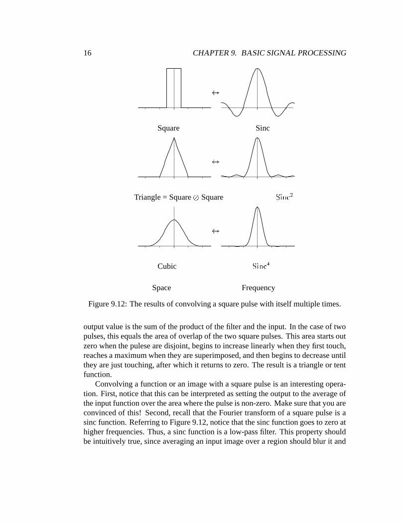
Figure 9.12: The results of convolving a square pulse with itself multiple times.

output value is the sum of the product of the filter and the input. In the case of twopulses, this equals the area of overlap of the two square pulses. This area starts outzero when the pulese are disjoint, begins to increase linearly when they first touch,reaches a maximum when they are superimposed, and then begins to decrease untilthey are just touching, after which it returns to zero. The result is a triangle or tentfunction.

Convolving a function or an image with a square pulse is an interesting opera-tion. First, notice that this can be interpreted as setting the output to the average ofthe input function over the area where the pulse is non-zero. Make sure that you areconvinced of this! Second, recall that the Fourier transform of a square pulse is asinc function. Referring to Figure 9.12, notice that the sinc function goes to zero athigher frequencies. Thus, a sinc function is a low-pass filter. This property shouldbe intuitively true, since averaging an input image over a region should blur it and

17

remove high frequencies.What is the spectrum of the function resulting from convolving two square pulses?

Convolving two functions corresponds to multiplying their spectra, therefore, con-volving a square pulse with a square pulse corresponds to the multiplication of twosinc functions. Similarly, the convolution of + pulses corresponds to the sinc raisedthe the n’th power. The function produced by convolving a pulse with itself + timesis called a B-spline. We will encounter B-splines again when discussing methodsfor representing curves and surface. Another interesting fact is that in the limit as +goes to infinity the convolution of + pulses approaches a Gauusian,

The convolution theorem states that multiplying two spectra in the frequency do-main corresponds to convolving the functions in the space domain.�G�� S ��Because the Fourier transform and the inverse Fourier transform are so similar, asymmetric interpretation is also true. That is, multiplying two functions in the spacedomain corresponds to convolving the functions in the frequency domain.� � � � S � �Sampling and Reconstruction

With this background on frequency space and convolution, we can now analyze theprocesses of sampling and reconstruction.

In the space domain, sampling can be viewed simply as multiplying the signalby sequence of spikes with unit area. Since the spikes are zero everywhere exceptat integer values, this has the result of throwing away all the information except atthe sample points. At the sample points, the result is the value of the function atthat point. This view of sampling in the space domain is illustrated in the top halfof Figure 9.13.

Additional insight into the sampling process, however, can be gained by con-sidering sampling in the frequency domain. Recall the convolution theorem. Thistheorem states that multiplying two signals in one domain (in this case, the spacedomain) corresponds to convolving the signals in the other domain (the frequencydomain). Thus, multiplying the function by a sequence of spikes in the space domaincorresponds to convolving the spectrum of the original function with the spectrumof a sequence of spikes. However, recall that the Fourier transform of a sequence ofspikes is itself a sequence of spikes. Thus, in the frequency domain, sampling corre-sponds to convolving the spectrum of the function with a sequence of spikes. Con-volving with a sequence of spikes causes the original function to be replicated—a


� ,

Sampling in the Space Domain

� ,

Sampling in the Frequency Domain

Figure 9.13: Sampling

19

� ,

Reconstruction in the Frequency Domain

� ,

Reconstruction in the Space Domain

Figure 9.14: Reconstruction

new copy of the spectrum is centered at a spike. The view of sampling in the fre-quency domain is illustrated in the bottom half of Figure 9.13.

Now let us consider the reconstruction process. The process of recovering theoriginal signal from the sampled signal is easiest to analyze in the frequency domain.Remember, the sampling process resulted in the replication of the spectrum of theoriginal function. If these replicas do not overlap, then the original can be recoveredby the application of a perfect low-pass filter. Multiplying the replicated spectrumby a square pulse centered on the original signals spectrum will remove all the extracopies of the spectrum. This is illustrated in Figure 9.14.

Of course, for every process in one domain we can create a dual process in the


� �

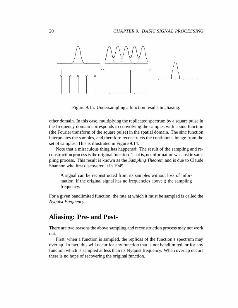
Figure 9.15: Undersampling a function results in aliasing.

other domain. In this case, multiplying the replicated spectrum by a square pulse inthe frequency domain corresponds to convolving the samples with a sinc function(the Fourier transform of the square pulse) in the spatial domain. The sinc functioninterpolates the samples, and therefore reconstructs the continuous image from theset of samples. This is illustrated in Figure 9.14.

Note that a miraculous thing has happened: The result of the sampling and re-construction process is the original function. That is, no information was lost in sam-pling process. This result is known as the Sampling Theorem and is due to ClaudeShannon who first discovered it in 1949.

A signal can be reconstructed from its samples without loss of infor-mation, if the original signal has no frequencies above

9� the samplingfrequency.

For a given bandlimited function, the rate at which it must be sampled is called theNyquist Frequency.

Aliasing: Pre- and Post-

There are two reasons the above sampling and reconstruction process may not workout.

First, when a function is sampled, the replicas of the function’s spectrum mayoverlap. In fact, this will occur for any function that is not bandlimited, or for anyfunction which is sampled at less than its Nyquist frequency. When overlap occursthere is no hope of recovering the original function.

21

Figure 9.16: Sampling a sine wave. Sampling the function �� 4 K H @&� yields the samevalues as sampling the function �� * K H @&� . Thus, the higher frequency 4 K H @ whichis above the Nyquist frequency, cannot be distinguished from the lower frequency* K H @ .

� �

Figure 9.17: Poor Reconstruction results in aliasing.

If copies of the spectra overlap, then some frequencies will appear as other fre-quencies. In particular, high frequencies will foldover and appear as low frequen-cies. This sudden appearance of some frequencies at other frequencies is referred toas aliasing. The result of the foldover is that the reconstruction process can not dif-ferentiate between the original spectrum and the aliased spectrum, and, hence, thefunction cannot be perfectly reconstructed. This effect is shown in Figure 9.15.

To illustrate aliasing consider the following thought experiment. Consider a sinewave with a frequency of 1.5 cycles per sample. Now sample the sine wave. Thissampling rate is less than the frequency of the function, and hence we may expectaliasing to result. This is seen in Figure 9.16. That figure shows that sampling �� ")# 4 K H ��yields the same values as sampling �� ")#�* K H �� .


Implicit in the sampling theorem is that the function be perfectly reconstructed.Unfortunately, this is often not possible in practice. For one, the perfect low-passfilter is a �� = function. However, convolving the sampled with a sinc function isimpractical because the �� = function has infinite extent. Also, in general, recon-struction is a property of the hardware and media. For example, most displays em-ploy a two step process. In the first step the digital value is converted to an analogvalue using a D/A convertor. Most D/A convertors sample the input and hold themconstant until the next input is available. This corresponds to convolving the sam-pled signal with a square pulse. In the second step the analog voltage is converted tolight using phosphors on the monitor. Most phosphors emit a small Gaussian spot oflight centered at the location of the electron beam. This has the effect of convolv-ing the signal with a Gaussian. Although the combination of these two steps is alow-pass filter, the filtering is not perfect.

This is illustrated in Figure 9.17. Suppose the function is reconstructed with asquare pulse. That would correspond to multiplying its spectra times the transformof the pulse—a �� = . However, a �� = does not perfectly remove all the replicas ofthe spectra produced by the sampling process, and so aliasing artifacts would be vis-ible.

In both these cases, frequencies may masquerade as other frequencies. The firstcause—due to undersampling—is called pre-aliasing; the second cause—due to badreconstruction—-is called post-aliasing.

Date post:	06-May-2018
Category:	Documents
Upload:	vucong
View:	250 times
Download:	2 times

Chapter 9 Basic Signal Processing - cs.princeton.edu 9 Basic Signal Processing ... Digital Signal...

Documents