Chapter 9GRASS GIS

M. Neteler, D.E. Beaudette, P. Cavallini, L. Lami and J. Cepicky

Abstract GRASS is a full featured, general purpose Open Source geographic infor-mation system (GIS) with raster, vector and image processing capabilities. There hasbeen constant development of the software since 1982, with recent major improve-ments reflecting renewed efforts by the international development team to make itone of the core components of the Open Source geospatial software stack. It canhandle 2D and 3D raster data, includes a topological 2D/3D vector engine, networkanalysis functions, and SQL-based attribute management. This chapter presents anoverview and practical examples of the GRASS 6 capabilities relevant to environ-mental and planning applications including new functionality. Enhancements to 3Dvisualization and approaches to environmental models are also discussed, as well asimage processing routines pertaining to LIDAR and multi-band imagery. Integra-tion of GRASS with other Open Source software packages for geostatistical analy-sis, cartographic output and Web GIS applications are described. Trends for futuredevelopment are also discussed.

M. NetelerFondazione Mach - Centre for Alpine Ecology, 38100 Trento (TN), Italy,e-mail: neteler@osgeo.org

D.E. BeaudetteDepartment of Land, Air and Water Resources, University of California, Davis, CA 95616, USA,e-mail: debeaudette@ucdavis.edu

P. CavalliniFaunalia, Piazza Garibaldi 5, 56025 Pontedera (PI), Italy, e-mail: cavallini@faunalia.it

L. LamiFaunalia, Piazza Garibaldi 5, 56025 Pontedera (PI), Italy, e-mail: lami@faunalia.it

J. CepickyHelp Service - Remote Sensing s.r.o., Cernoleska 1600, 25601 - Benesov, Czech Republic,e-mail: jachym.cepicky@gmail.com

G.B. Hall, M.G. Leahy (eds.), Open Source Approaches in Spatial Data Handling. 171Advances in Geographic Information Science 2, c© Springer-Verlag Berlin Heidelberg 2008

172 M. Neteler et al.

9.1 Introduction

The Geographic Resources Analysis Support System (GRASS, http://grass.osgeo.org) was born in the early 1980s at the Construction Engineering Research Labora-tory (CERL) of the United States Army as a software management tool for militaryapplications. It has evolved into one of the most comprehensive, general purposefree and open source for geospatial (FOSS4G) systems in existence. GRASS is araster/vector geographic information system (GIS) combined with integrated imageprocessing and data visualization subsystems. It includes hundreds of modules formanagement, processing, analysis and visualization of geo-referenced, spatial data.It includes unique algorithms and methods that are implemented in a portable en-vironment making it one of the few GIS in the world that works under a varietyof different operating systems and platforms. GRASS is fundamentally a desktopGIS, however recent efforts are in place to extend functionality to Web-based andnetwork-programmable interfaces.

The limitations of computer hardware in the early 1980s, coupled with the in-novation of skilled and motivated young researchers lead to a first working versionof GRASS. It was designed as a modular system written in the C programminglanguage. The advent of the Internet facilitated the spread of the software amonguniversities and other governmental organizations. As CERL and GRASS evolvedthrough the late 1980s and early 1990s, CERL created the Open GRASS Founda-tion which evolved into the Open GIS Consortium (OGC, now known as the OpenGeospatial Consortium). The discontinuation of development of GRASS by CERLin 1996 lead to the formation of the GRASS Development Team two years later.

A first release as Free Software under the GNU General Public License (GPL)was published in October 1999. Based on academic efforts, GRASS is today devel-oped by a worldwide group of scientists, programmers, power users and enthusiasts.The project is attractive to a new generation of users and developers due to the mod-ernization of the software. The release of GRASS 6 reflects new efforts to one of thecore components in the FOSS4G software stack. Quality management is enforcedby transparent development methods such as a centralized source code repository(in a concurrent versions system (CVS) server) and the immediate peer-review ofsource code changes by email broadcast.

In 2006, the Open Source Geospatial Foundation (OSGeo, http://osgeo.org) wascreated to bundle several FOSS4G software projects, including GRASS, into a jointorganization. This chapter presents an overview of the GRASS 6 capabilities rel-evant to environmental and land management applications, including the updatedand new tools for 2D and 3D raster data, the vector modules based on the re-designed topological 2D/3D vector engine, and SQL-based attribute management.Approaches to linking with other FOSS4G tools and environmental models are alsodiscussed.

9 GRASS GIS 173

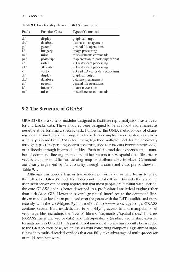
Table 9.1 Functionality classes of GRASS commands

Prefix Function Class Type of Command

d.∗ display graphical outputdb.∗ database database managementg.∗ general general file operationsi.∗ imagery image processingm.∗ misc miscellaneous commandsps.∗ postscript map creation in Postscript formatr.∗ raster 2D raster data processingr3.∗ 3D raster 3D raster data processingv.∗ vector 2D and 3D vector data processingd.∗ display graphical outputdb.∗ database database managementg.∗ general general file operationsi.∗ imagery image processingm.∗ misc miscellaneous commands

9.2 The Structure of GRASS

GRASS GIS is a suite of modules designed to facilitate rapid analysis of raster, vec-tor and tabular data. These modules were designed to be as robust and efficient aspossible at performing a specific task. Following the UNIX methodology of chain-ing together multiple small programs to perform complex tasks, spatial analysis isusually performed in GRASS by linking together multiple modules either directlythrough pipes (an operating system construct, used to pass data between processes),or indirectly through intermediate files. Each of the modules expects a small num-ber of command line arguments, and either returns a new spatial data file (raster,vector, etc.), or modifies an existing map or attribute table in-place. Commandsare clearly organized by functionality through a command class prefix shown inTable 9.1.

Although this approach gives tremendous power to a user who learns to wieldthe full set of GRASS modules, it does not lend itself well towards the graphicaluser interface-driven desktop application that most people are familiar with. Indeed,the core GRASS code is better described as a professional analytical engine ratherthan a desktop GIS. However, several graphical interfaces to the command line-driven modules have been produced over the years with the TclTk toolkit, and morerecently with the wxWidgets Python toolkit (http://www.wxwidgets.org). GRASScontains several libraries dedicated to simplifying access to and manipulation ofvery large files including, the “rowio” library, “segments”/“spatial index” libraries(GRASS raster and vector data), and interoperability (reading and writing externalformats such as GeoTIFF). A parallelized numerical library has recently been addedto the GRASS code base, which assists with converting complex single-thread algo-rithms into multi-threaded versions that can fully take advantage of multi-processoror multi-core hardware.

174 M. Neteler et al.

9.2.1 Installation

GRASS software can be downloaded freely from the main GRASS Web site(http://grass.osgeo.org). This site is mirrored in several countries for faster access,including the United States GRASS mirror at http://grass.ibiblio.org. Source code(the portable version for all operating systems) as well as the latest ready-to-installbinaries for GNU/Linux, MacOSX and MS-Windows (native or optionally with theCygwin tools) are all available on this site. GRASS is also available on CDROM/DVD from various providers. The MS-Windows version of the popular QuantumGIS (QGIS, http://qgis.org) package includes a native GRASS installation. QGIS isa user friendly geographic data viewer with some analytical capabilities that runs onGNU/Linux, Unix, MacOSX, and MS-Windows. It supports vector, raster, databaseformats, OGC Web Services and includes a GRASS toolbox. QGIS is licensed underthe GNU GPL.

9.2.2 Functionality and Command Structure

GRASS contains over 300 programs and tools to render maps and images both on-screen and on paper, to manipulate raster and vector data, to process multi spectraland time series image data, and to create, manage, and store spatial data. As notedearlier, GRASS uses both an intuitive graphical user interface as well as commandline syntax for ease of operations. Approximately 200 of the modules that are avail-able in GRASS GIS are integrated in pull down menus. The most frequently usedmodules can thus be easily accessed with the use of a mouse.

GRASS 6 introduces a new topological 2D/3D vector engine and support for vec-tor network analysis. Attributes are managed in DBF files or a SQL-based databasemanagement system (DBMS). The NVIZ visualization tool displays raster data, 2Dand 3D vector data as well as voxel volumes. GRASS project databases (“locations”)can be auto-generated by a European Petroleum Survey Group (EPSG) code numberor from geo-coded data sets. GRASS is fully integrated with GDAL/OGR librariesto support an extensive range of raster and vector data formats (see Chap. 5 of thisbook), including the OGC Simple Features specification. To facilitate usage by non-English speakers, user messages have been translated to various languages includingAsian languages. GRASS supports work groups through its LOCATION/MAPSETdirectory structure concept which can be set up on shared/network disk devices.Through this, team members can simultaneously work in the same project’sdatabase.

9.3 GRASS Features

Although GRASS has evolved into a general purpose GIS, its major strength re-mains environmental modeling and analysis. With respect to older versions, signifi-

9 GRASS GIS 175

cant improvements have been implemented to strengthen its viability. In this regard,interoperability is seen as a crucial element in GRASS development, leveragingfrom widely used data exchange libraries. Key motivations for using the softwareare its strong analytical capabilities for both raster and vector data (in 2D and 3Dspace) as well as graphical data exploration and visualization.

9.3.1 Data Exchange: Interoperability

GRASS data are maintained in their own directory structure in so-called “locations”and “mapsets”. The idea behind this structure is to provide a multi-user environmentwith access control. Locations can be maintained on a centralized server. Extensivecapabilities of data exchange are essential for daily GIS work. For interoperability,GRASS profits from an external project, the GDAL/OGR library, which allows theconversion among many raster and vector formats, including the internal GRASSformats. This library is also used by global data vendors as well as in some pro-prietary GIS applications. Additional GRASS modules allow importing from andexporting to other formats.

GRASS uses a topological vector architecture. To support Simple Features vectordata (conformal to OGC standards), these data sets are converted upon data import.Conversely, export into Simple Features is also possible. Instead of importing datasets, vector maps may also by linked to the GRASS database as virtual maps. Themodule for importing vector maps, v.in.ogr, uses the OGR library (for a full list ofsupported formats, see the GDAL/OGR Web site, http://www.gdal.org/). This mod-ule also allows merging of a series of different vectors, limiting the import to auser defined spatial subset, and creating a new GRASS location on the basis of theprojection system of the imported data. Additional modules allow the managementof a variety of data formats, including ASCII files, 2D and 3D drawings from com-puter assisted design (CAD) software, common vector formats, Gazetteer and globalpositioning system (GPS) data, as well as data import from Web Feature Services(WFS).

The r.in.gdal module, which uses the GDAL library, enables raster datasets tobe imported. The module also allows the import of single bands from multi-bandimagery, and the creation of a new GRASS location from the imported dataset.Additional modules allow the import of various ASCII and binary files including allcommon raster and imagery formats including elevation models, aerial and satelliteimagery, and data from Web Mapping Services (WMS). It is also possible to create3D raster maps from 2D map slices, or from importing 3D volume files.

Once in GRASS, raster maps can be converted to vector maps and vice versa.Vector geometries can also be converted between different types (points, lines, poly-gons), and a series of raster layers can be transformed into raster volumes and viceversa. 3D points can also be converted or interpolated to raster volumes. Exportingfiles is essentially similar, with the same formats supported (with minor differences).GRASS raster and vector maps can be exported also to rendering software (e.g.,POV-Ray or Paraview). 3D fly-throughs can be created as MPEG format animations.

176 M. Neteler et al.

9.3.2 Raster Data Analysis: Pixels and Voxels

Raster analysis is the historical core of the GRASS project. In addition to 2Draster maps (pixel-based), GRASS can also manage 3D (volume) raster maps(voxel-based). Many modules are available for raster processing, and they can besubdivided into the following groups:

• Map management: editing, extent, management of null values, resampling, re-projecting etc.;

• Colour management: setting colour tables, weighted merging and splitting ofRGB/HIS and normal maps;

• Buffer creation: single and multiple buffers;• Mask creation: to apply analyses to a limited subset of the working map;• Proximity analysis: analysis through a moving window to create maps in which

every cell is the result of a function applied to the surrounding cells; calculationof minimum distances among raster objects;

• Map overlay: statistics, temporal series, patching maps, etc.;• Solar radiance and shadowing: calculation of solar irradiation and shadows on

the basis of date and time;• Terrain analysis: calculation of total cumulative cost of movement over a digital

terrain model (DTM) or a cost map, search of a minimum cost path, profile anal-ysis, calculation of exposure and slope maps, texture analysis, visibility analysis;

• Raster transformation: finding islands of contiguous cells of the same type, grow-ing and linearizing raster islands;

• Specialized models: hydrology, landscape ecology, fire spread;• Reclassification: on the basis of user rules, of island size, recoding and rescale;• Random raster maps: generating raster points (also on the basis of a second raster

map);• Surface generation: density maps (kernels) from vector points, planes, fractal

surfaces, Gaussian derivates, random surfaces with spatial dependency;• Surface interpolation: bilinear, bicubic, inverse distance weighted (IDW), and

regularized splines with tension (RST);• Reports and statistics: general statistics, correlation and linear regression be-

tween raster maps.

GRASS raster map processing is always performed in the current region settings.That is, the current region extent and current raster resolution is used. If the resolu-tion differs from that of the input raster map(s), on-the-fly re-sampling is performed(nearest neighbour re-sampling). If this is not desired, the input map(s) has/have tobe re-sampled beforehand with one of the dedicated modules. GRASS applies twogeneral rules in this context:

1. Raster/imagery output maps have their bounds and resolution equal to those ofthe current region.

2. Raster/imagery input maps are automatically cropped/padded and rescaled (usingnearest-neighbour resampling) to match the current region.

9 GRASS GIS 177

9.3.3 Vector Data Analysis

The vector engine of GRASS has been completely overhauled during the lastfew years. Geometry and attribute management are clearly separated, giving moreflexibility in data storage. The vector geometry was extended to manage 2D and3D vector data. Vectors are fully topological, with spatial relationships (e.g., con-nection, adjacency, inclusion) embedded in the information linked to each vectorelement. For instance, a border line between two polygons is not replicated, but issingular, and linked to the left- and right-sided polygon centroids. This new internalvector data format is also portable across 32bit and 64bit platforms.

A new spatial index system as well as category index accelerates data access. Thesupport of topology enables the user to perform data cleanup to ensure data consis-tency. Support for vector map overlays, intersections and extraction of features isimplemented. A new digitizing tool permits users to create or update vector featureswith attributes on-screen. The attribute management includes full and flexible inte-gration of database management systems (PostgreSQL, MySQL, DBF, SQLite andODBC are currently supported). Structured query language (SQL) statements, usedto manage attributes, are directly passed to the underlying database system. The setof supported SQL commands depends on the RDMBS and selected driver. Graph-ical updating of vector attributes has been implemented as well. Available vectordata types are:

• Point: a single data location;• Line: a directed sequence of connected vertices with two endpoints called nodes;• Boundary: the border line to describe an area;• Centroid: a point within a closed boundary;• Area: the topological composition of centroid and boundary;• Face: a 3D area;• Kernel: a 3D centroid in a volume (in development);• Volume: a 3D corpus, the topological composition of faces and kernel (in devel-

opment).

GRASS vector maps may include different vector types (points, lines, areas etc.)in the same layer. Available vector analysis methods are quite advanced, and arecategorized into several groups:

• Map management: editing, topology rebuilding, cleaning up of non-topologicalimported vectors, adding centroids to polygons, merging and splitting of ele-ments, geometry conversions (2D and 3D; rebuilt on the basis of a DTM; extru-sion), re-projection;

• Attribute management: connecting vectors to attribute tables (on various databasebackends);

• Reports and statistics: general statistics, export of geometric characteristics todatabase, normality tests on point distribution, correlation of values and corre-sponding raster cells;

178 M. Neteler et al.

• Extraction and selection: on the basis of a geometry or a table query, selectionof a vector on the basis of the relations with the geometries of another vectorbuffer;

• Proximity analysis: calculation of minimum distance matrix among objects;• Map overlay: patching and overlaying vectors, management of attributes;• Generation of reference maps: creation of grids of polygons or points;• Reclassification: management and reclassification of categories associated to

geometries;• Points: import of point vectors from an x,y[,z] table, creation of random points,

minimum convex polygons, Voronoi tessellation and Delaunay triangulation,raster values extraction;

• Lidar data analysis: outlier detection, Digital Surface model (DSM) and DTMseparation and interpolation;

• Network analysis: creation of a network, finding the shortest path, allocation ofsub-nets for nearest centers, Steiner tree, or resolution of the traveling salesmanproblem;

• Linear referencing system: creation, editing and management.

9.3.4 Attribute Data Storage via a DBMS

GRASS provides tools for management and analysis of vector maps, including theattributes that can be stored in a DBMS. GRASS can be connected to various re-lational DBMS (RDBMS) and embedded databases. It supports SQL to create, re-trieve, update, and delete data from RDBMS. GRASS unifies the different driversin an abstraction layer named the database management interface (DBMI) to assistthe user.

Usually an attribute table is linked to vector geometry data. The attribute tablemust contain a column named “cat” to store the category numbers (the vector IDs)which connect the individual vector objects to attributes. Each table row correspondsto a category number. Several vector objects can be assigned to the same categorynumbers (table row).

It is possible to link the geographic objects in a vector map to one or more tables.Each link to a distinct attribute table is called a layer. A link defines the databasedriver, the database name, and the table name that are used. Each category numberin a geometry file corresponds to a row in the attribute table. Using v.db.connect,layers can be listed or maintained. GRASS layers do not contain any geographicobjects, but they consist of links to attribute tables in which vector objects can havezero, one, or more categories. If a vector object has zero categories in a layer, thenit does not appear in that layer. Some vector objects may appear in some layers butnot in others. The practical benefit of this approach is that it allows placement ofthematically distinct but topologically related objects into a single map (e.g., forestsand lakes). These virtual layers are also useful for linking time series attribute datato a series of locations that do not change over time. By default the first layer is

9 GRASS GIS 179

... ...

layer1 layer2 geometry

cat1 cat1cat2 cat2cat8 cat4

cat attrib1 attrib2 attrib3 ...

... ... ...

1 lulc1 a12 lulc2 b1

4 ... ...

cat attrib1 attrib2 attrib3 ...

1 soil1 4.62 soil2 5.4

8 ... ...... ... ...

GeometryTable 1 Table 2

Fig. 9.1 Example for layer concept in GRASS vector files: geometry file with two layers connectedto two different attribute tables (linking field “cat”)

active (i.e., the first table corresponds to the first layer). Further tables are linkedto subsequent layers. Figure 9.1 illustrates the layer concept with an example for avector map with two layers, connecting two different attribute tables to the vectorgeometry.

9.3.5 Visualization: 2D, 3D and Animations

Besides the creation of 2D maps, GRASS also provides the possibility to create im-pressive 3D visualizations and animations of surfaces and volumes using the NVIZmodule (Fig. 9.2). This module uses raster data to define both height and attributedata, and to allow the overlay of vector data (points, lines and areas). It also has il-lumination tools to add shadow effects. After starting NVIZ, a graphic window anda control window are opened, and the individual features are displayed. A series ofimages can be saved and combined into a GIF animation or an MPEG movie file viaexternal programs. This is especially interesting when analyzing changes over time.

(a) (b)

Fig. 9.2 Some examples of how NVIZ displays both volumetric (a) and conventional 3D (b) rasterand vector data types

180 M. Neteler et al.

9.4 Raster Applications

Given the raster data processing origins of GRASS, it is not surprising that the rastermodules are among the oldest and best developed in its toolbox. Several commonapplications of the GRASS raster modules such as surface analysis, geomorphome-tric classification, interpolation, and solar radiation modeling are included in thissection. A more complete discussion of these modules can be found in Neteler andMitasova (2008).

9.4.1 Cost Surface Analysis: Wilderness Navigation

Cost surface analysis is a method of automatically identifying a path which mini-mizes the amount of accumulated “cost” between a series of points. Conceptually,this approach is very similar to the actions of a mountain hiker seeking to mini-mize the total change in slope encountered while traversing an area. It follows theprinciple that walking up or down steep hills is hard, and walking a long distanceup or down a steep slope is even harder. In GRASS, the modules r.cost and r.walkare used to compute accumulated cost from some start point to an end point. Themodule r.drain is then used to identify the path of least cost between end and startpoints, akin to the movement of a drop of water down an elevation gradient. A slopemap is commonly used as an input to r.cost. However, more complex systems canbe modeled by altering a slope map with r.mapcalc.

Consider the example of a trip through rugged terrain between numerous sub-alpine lakes. The region is mostly wilderness, and therefore trails are few and donot directly connect specific lakes that fall along a desired route. Identifying thepaths between points of interest which minimize slope traversal has been done withpaper topographic maps for decades. Cost surface analysis is well suited to this typeof problem. For example, the task of navigating between Bill Lake and Bonnie Lakeshown in Fig. 9.3(a) is a good case in point. In this example, additional sources of“cost” are added to the slope map as follows:

• traversing lakes is not acceptable (extreme travel cost added to slope map);• traversing wooded areas is faster due to shading (moderate travel cost subtracted

from slope map).

By specifying start and stop points, along with the composite travel “cost” map,the least-cost path between these points can be computed via the GRASS com-mands r.cost and r.drain. It is possible to see how r.drain actually simulates theflow of a drop of water down an elevation surface in an energy minimizing oper-ation (Fig. 9.3(b)). However, in this case, the elevation surface is actually a travelcost map (computed by r.cost). The path of the theoretical drop of water repre-sents the least-cost route from the starting point to the end point. Note that the startpoint for r.cost (point of origin) is actually the end point for r.drain. By specifyingvery large travel costs for traversing lakes (peaks), and slightly lower travel costsfor wooded areas, the computed least cost path goes “around” lakes and “through”wooden areas.

9 GRASS GIS 181

(a) (b)

Fig. 9.3 An example least-cost path calculation. A hiker wishes to travel from Bill Lake to BonnieLake (a); the accumulated cost surface and least-cost path between the two points (b)

9.4.2 Interpolation Functions

GIS are often used to interpolate continuous raster surfaces from regularly, irreg-ularly, or even scarcely distributed point data. These surfaces usually represent el-evations, temperatures, or other continuous phenomena. Interpolations can also beperformed from contour data. Re-sampling to a different resolution can also be seenas a special case of interpolation.

GRASS supports a range of re-sampling and interpolation methods such asnearest neighbour re-sampling, bilinear and bicubic interpolation (r.resamp.interp),inverse distance weighted (IDW in v.surf.idw, Lo and Yeung 2006; Issaks andSrivastava 1989) and regularized splines with tension (RST) in v.surf.rst as wellas v.vol.rst for volumetric data (Mitasova and Mitas 1993; Mitasova and Hofierka1993).

Data interpolation in GRASS is explained in detail in Neteler and Mitasova(2008). The RST method especially gives much control over the behaviour of the in-terpolator through the smoothness and tension parameters. To obtain reasonable re-sults, an integrated cross-validation algorithm helps to find input parameters whichminimize the interpolation error. Integrated segmentation allows interpolation ofmassive data sets. Additional related methods are re-sampling of point data andraster maps using spatial aggregation (r.in.xyz and r.resamp.stats) and temporal ag-gregation (r.series).

9.4.3 Geomorphological Analysis

Landscape processes, including water and sediment flow, are both caused and influ-enced by the geometry and properties of the land surface. Basic land features (e.g.

182 M. Neteler et al.

planes, pits, peaks, ridges etc.) can be identified with the module r.param.scale.GRASS includes also an extensive set of modules for deriving land-surface pa-rameters and performing spatial analysis that involves elevation data (Hofierkaet al. 2008).

Fundamental parameters of the surface can be calculated using partial derivativesof the mathematical function describing the surface as local parameters (based on apoint and its immediate surroundings):

• Slope (steepest angle of the slope);• Aspect (slope orientation, direction of gradient, steepest slope or flow direction);• Profile curvature (surface curvature in the direction of gradient);• Tangential curvature (surface curvature in the direction of contour tangent);• Mean curvature (an average of the two principal curvatures).

Additionally, GRASS provides a wide array of tools to analyze water flow andwatershed parameters, starting from basic parameters (flow accumulation, upslopecontributing area, stream network, watershed (basin) area, flow path length) to com-plex algorithms for flow routing:

• Single flow direction to eight neighbouring cells moves flow into a single down-slope cell (r.watershed);

• Single flow to any direction (D-inf or vector-grid approach) (r.flow);• Multiple flow direction (MFD) to two or more down slope directions (r.terraflow,

r.topmodel);• 2D water movement simulation based on overland flow differential equations

(r.sim.water).

Various models and parameters can be combined, and new models can be devel-oped through the use of the map algebra module r.mapcalc.

9.5 Vector Applications

The GRASS vector model contains a description of topology. From the user’sperspective, topological operations enable verification and enforcement of dataintegrity and quality. By default, GRASS 6 always builds the topology after im-porting, creating or modifying a map. A considerable amount of detail about thesealgorithms can be found in the relevant literature (Lo and Yeung 2006; Neteler andMitasova 2008)

9.5.1 Overlay Operations and Selections

Geometric operations are performed through specialized modules. By selecting anoperator, features from two input maps are geometrically elaborated and the result iswritten to a new output vector map. A typical set of operators and tools are available:

9 GRASS GIS 183

• and: also known as “intersection”;• or: also known as “union”;• not: features from map A not overlaid by features from map B;• xor: features from either map A or map B but not those from A overlaid by B;• point-in-polygon selection;• vector extraction (spatially, or based on SQL statements).

9.5.2 Network Analysis and Linear Reference System

The integrated Directed Graph Library (DGL) provides support for vector networkanalysis. Available algorithms include shortest path, traveling salesman (round trip),allocation of sources (sub-networks), Minimum Steiner Trees (star-like connec-tions), and iso-distances (from centres). Costs may be assigned both to nodes andarcs. Both directions of a vector line can be used, which permits definition of a for-ward and a backward direction, and storing of their attributes in the related attributetable. An example for shortest path routing on a vector network is shown in Fig. 9.4.

The following modules are available:

• Shortest-Path Analysis: the commands d.path and v.net.path allow calculation ofthe least expensive (by default the shortest path as the length of the vectors is usedas the measure of cost) distance between two chosen points with two methods.Additional information about the vectors (e.g., speed limit on the road or roadstatus) can be used for calculating a path. Cost information can also be assigneddifferentially to both vector directions. Attributes of the nodes (e.g., cycle timesof the traffic lights at a crossroad) can also be considered.

• Subnets within a vector network: a given vector network can be subdivided intosub-networks with the module v.net.alloc. For instance, regions in a city can beidentified that are best served by a limited number of fire stations.

Fig. 9.4 Simple example of a shortest-path calculation from node 1 (green square) to node 2 (redcircle) along a network

184 M. Neteler et al.

• Minimum Steiner Tree problem: the optimal connection of nodes within a net-work (star) can be described by the Minimum Steiner Tree. For instance, sev-eral hospitals distributed in a region need new fibre-optical network cables fortelemedical services. The aim is to lay the necessary cable along existing roads,while using the least amount of cable to connect all hospitals. The GRASS mod-ule v.net.steiner is used for this purpose.

• Traveling-Salesman problem: the classic problem of calculating the best routejoining a series of points (either by distance or time) can be solved with theGRASS module v.net.salesman. As an example, a route minimizing cost for acompany representative visiting a series of customers can be calculated.

• Cost analysis: finding iso-distances (concentric distances around a series ofpoints) on a network can be performed with the GRASS module v.net.iso. Forinstance, “run-length” (e.g. for sewage channel systems) can be calculated basedon the vector length or, as in previous modules, other attributes. Another applica-tion is the search for reachable points of interest within a five minute walk froma metro-station.

Besides vector networking, GRASS also supports Linear Reference Systems(LRS; Blazek 2005). A LRS is a system where features (points or segments) arelocalized by a measure along a linear element. The LRS can be used to refer-ence events for any network of linear features, for example roads, railways, rivers,pipelines, electric and telephone lines, water and sewer networks. An event is de-fined in LRS by a route ID and a segment. A route is a path on the network, usuallycomposed from more features in the input map. Events can be either points or linesegments.

9.5.3 LIDAR Data Processing

Airborne Light Detection and Ranging (LIDAR) is one of the most recent tech-nologies in surveying and mapping. A laser on board a plane sends out pulses tothe ground in order to determine the distance to an object or surface. This distanceis determined by measuring the time delay between transmission of a pulse anddetection of the reflected signal. The horizontal and vertical accuracies are in thecentimetre range. Up to four range measurements can be performed for each pulse.LIDAR offers various new applications including terrain change analysis to studyvertical and horizontal changes in terrain (e.g. beaches) and allowing for calculationof area and volume change. Another application is hazard mapping (e.g. detectionof avalanches or other morphological hazards). In the area of energy analysis, solarenergy can be estimated at building detail for alternative energy evaluation, sinceroof inclination and structure details can be derived from LIDAR data. The LIDARtoolset in GRASS provides advanced methods to compute the digital surface (DTMor DSM) based on radial basis functions and spline functions with the Thykhonovregularizer (Brovelli et al. 2004).

9 GRASS GIS 185

The data elaboration procedure is started with the import of LIDAR point clouds(first and last pulse) with v.in.ascii. In this case, the topology is not built to avoidredundant computations. Subsequent outlier detection is done with v.outlier on bothfirst and last pulse data. At the next step, edges are detected from the last pulsedata with v.lidar.edgedetection. The DSM (buildings, vegetation etc.) is generatedwith v.lidar.growing from detected edges. The resulting data are post-processed withv.lidar.correction. Finally, the DTM and DSM are generated with v.surf.bspline.

The r.in.xyz module can be used to perform binning of points derived fromraw sensor measurements, or coordinates exported from the common AmericanSociety for Photogrammetry and Remote Sensing LIDAR Exchange Format (LAS),to grid cells of a given size. This module can use several common statistics suchas min, max, mean, and range for cell-wise aggregation. With careful tuning of re-gion settings (extent and resolution), it is possible to generate grid point data wherethe number of features exceeds the practical limits imposed by the GRASS vec-tor engine. Tests have shown that r.in.xyz performs well with over 25 million inputfeatures.

9.6 Image Processing

Remote sensing is a rapidly advancing technology for gathering environmental datausing a wide range of airborne and satellite platforms, and it plays a major rolein spatio-temporal earth surface monitoring. Image data within GRASS are treatedidentically to raster data. However, several commands are explicitly dedicated toimage processing. GRASS supports import of common satellite data and imageryformats, geocoding of imagery data, visualizing (true) colour composites, calcula-tion of vegetation indices, calibration of channels, image classification and imagefusion as well as time series processing.

Satellite imagery and orthophotos (aerial photographs) are handled in GRASSas raster maps and specialized tasks are performed using the imagery (i.∗) modules.All general operations are handled by the raster modules.

9.6.1 Common Operations

Besides visualization, all common steps of radio and geometric pre- and post-processing are supported. Some of the available techniques are illustrated in thefollowing sub-sections.

9.6.1.1 Visualizing True Colour Composites

The GRASS command d.rgb can be used to combine the first three channels quicklyto a near natural colour image. The graphical GIS manager (gis.m) offers an easy

186 M. Neteler et al.

interface to work with colour composites. The procedure assigns each channel toa colour which is then mixed while displayed. With some user optimization of thegrey scales of the channels, nearly perfect natural colours can be achieved. Thei.landsat.rgb can be used to adjust automatically LANDSAT red, green, and bluechannels to closely match the colours perceived by the human eye. Channel his-tograms can be displayed with d.histogram. However, this command operates onany raster map.

9.6.1.2 Calculation of Vegetation Indices

A common proxy for chlorophyll content, utilizing both red (LANDSAT channel 3)and near infrared (LANDSAT channel 4) wavelengths, is the normalized differencevegetation index (NDVI; Jensen 2000). A NDVI map is commonly used to infer wa-ter stress in plants, vegetative intensity, or potential crop yields. Calculation of thisand other vegetation indices can be done in a single step with simple map algebra,as implemented in the GRASS command r.mapcalc:

ndvi = 1.0∗(tm4− tm3)/(tm4− tm3)

where:

ndvi the resulting map,tm3 and tm4 the LANDSAT channels existing as GRASS raster maps.

The command r.colors can be then used to create an optimized colourtable. The Kauth-Thomas “Tasseled Cap” transformation for LANDSAT-TM sen-sor data can be performed directly with the GRASS command i.tasscap. A com-prehensive list of vegetation indices and their respective formulae can be found inJensen (2000).

9.6.1.3 LANDSAT Operations

The encoded digital numbers of a thermal infrared channel can be transformed todegrees Celsius (or other temperature units) that represent the temperature of theobserved land surface. This requires a few algebraic steps with r.mapcalc whichare outlined in the literature to apply gain and bias values from the image metadata(Neteler and Mitasova 2008).

A downscaling approach commonly applied to channels 1, 2, 3, 4, 5, and 7(30 meter resolution) can be performed in GRASS with the Brovey transform(i.fusion.brovey) method. This approach fuses the panchromatic channel (15 metreresolution) with selected channels to produce a new “pan-sharpened” color com-posite at 15 metre resolution. Colour composites can be displayed with d.rgb, asdescribed earlier, or saved with r.composite.

9 GRASS GIS 187

9.6.1.4 Time Series Processing

GRASS also offers support for time series processing (r.series). Statistics can bederived from a set of co-registered input maps such as multi-temporal satellite data.Common univariate statistics and linear regressions can be calculated. For example,Rizzoli et al. (2007) used MODIS time series data processed in GRASS to pre-dict the highest risk areas for increased tick-borne encephalitis virus activity in theProvince of Trento, Italy.

9.6.1.5 Rectification/Ortho-Rectification

GRASS is able to geocode raster and image data of various types, including un-referenced scanned images of maps by defining four corner points, unreferencedsatellite data from optical and Radar sensors by defining a certain number of groundcontrol points (i.group, i.target, i.points, i.rectify), and orthophotography based onDEM data (i.ortho.photo). Also, digital photographs from handheld cameras can begeocoded using a modified procedure for i.ortho.photo (Neteler et al. 2005).

Geo-referencing in GRASS is done by first importing the images into a genericx,y (non-projected) location. Several bands of the same images can be treated to-gether, defining a group. The user is then prompted to identify a series of groundcontrol points. A Root Mean Square is automatically calculated during the process,providing a means to keep track of the overall accuracy while inserting points. Ref-erenced images are then transformed into a new geo-referenced location by polyno-mial transformation.

9.6.2 Image Classification

A thematic map can be generated from one or more input channels. These inputchannels are usually derived from aerial or satellite data. Multispectral data canbe considered as a stack of raster maps with identical spatial references. Duringthe image classification procedure the spectral response of objects is analyzed andassigned to classes. The resulting map contains a set of classes which may representland use or land cover. An example of unsupervised classification, performed withan IKONOS multi-band image is depicted in Fig. 9.5. Modules i.class and i.maxlikwere used for this analysis.

GRASS supports multiple channels which can be grouped together with thei.group module. Then either an automated statistical analysis can be performed onthe input channels (i.e., an unsupervised classification), or training areas can bedigitized by the user to define known land use/land cover areas (i.e., a supervisedclassification). GRASS derives spectral signatures for the desired classes and runsthe final analysis on all pixels of all input channels, assigning each pixel to a class.In the case of unsupervised classification, the classes are arbitrarily numbered, while

188 M. Neteler et al.

(a) (b)

Fig. 9.5 Unsupervised classification of an IKONOS 3-band pseudocolour image (a) into 5 discreteclasses (b)

in the case of supervised classification they correspond to the names of the trainingareas (Neteler et al. 2005).

Single and multispectral data can also be classified to user-defined land use/landcover classes. In the case of single channel data, segmentation or partitioning ofimages is used. GRASS supports the following methods:

• Radiometric classification;• Unsupervised classification (i.cluster and i.maxlik) using the Maximum Likeli-

hood classification method;• Supervised classification (i.gensig or i.class, i.maxlik) using the Maximum Like-

lihood classification method;• Combined radiometric/geometric (segmentation based) supervised classification

(i.gensigset, i.smap);• Kappa statistics can be calculated to validate the results with r.kappa.

Machine learning, the science of discovering and recognizing patterns in datawith algorithms that improve automatically through experience, has been frequentlyapplied to image processing in recent years. Based on samples, a classification orregression function is synthesized in order to predict unknown observations (forexample, for a land use/land cover classification). Several machine learning tech-nologies have been implemented in a new set of GRASS modules. The recentlyadded i.pr family of image processing modules implement several additional mod-ern classification routines including:

• k-NN (multiclass);• classification trees (multiclass);• maximum likelihood (multiclass);• support vector machines (binary).

Robust estimation of classes is gained with bagging and boosting. Feature nor-malization within each module allows for the inclusion of predictor variables with

9 GRASS GIS 189

non-normal distributions or different ranges. There is planned support for featureselection techniques such as re-sampling and cross-validation, for all classificationalgorithms available in i.pr.

9.7 GRASS Development

The FOSS4G concept offers a license scheme which defines the extent of the usage,modification, and redistribution of original and derived software. For GIS, unlimitedaccess to the source code is of particular interest, as the underlying algorithms areoften complex and have significant influence on the results of spatial analysis andmodeling. While an average user may not be able to trace errors within complexsource code, there are a number of specialists willing to test, analyze and fix anyerrors identified within the code. This framework is embedded into an Internet-based development model with a high frequency of new releases. The diversity inbackground and expertise of the developers contributes greatly to network synergy.Overall, this type of software development model leads to faster and more efficientproduction, along with stable and robust products.

9.7.1 The Development Model: Community-Based

Access to others who are using GRASS, and to the individuals who are activelymaintaining the GRASS code base is critical to the OS development model. SeveralGRASS-related mailing lists and Internet Relay Chat (IRC) channels serve as win-dows into the GRASS user base and development communities. Additionally, a bugand wish tracking system is used. New and seasoned users alike can find answers,submit bugs, or even contribute code and documentation suggestions through theseresources. This style of development fosters a two-way relationship between usersand developers. In many cases users find that over the course of a couple of yearsthey can progress from a simple interested party to a part-time contributor of doc-umentation and source code suggestions. Several of the core GRASS developmentteam have followed this path, and they are now in charge of a large and complexcode base.

The development tool set includes a server-based code repository with imme-diate change notification via email for peer-review of the changes. The GRASSProject Steering Committee (PSC) is responsible for granting write access to newdevelopers. To control and improve the source code quality, an automated code mon-itoring system was established to apply software engineering metrics and clone de-tection (i.e., identification of undesired source code copies which are identical orrather identical) on every change happening in the source code repository (Bouktifet al. 2006). This GRASS quality assurance system will be further improved andextended in the future and may potentially be made available to further projects un-der the auspices of the Open Source Geospatial Foundation (OSGeo) (see Chaps. 1and 2, among others, of this book).

190 M. Neteler et al.

9.7.2 GRASS Programming

GRASS provides a unique opportunity to improve and extend basic GIS capabilitiesthrough new code development and the support of the GRASS developer commu-nity. The complete GRASS source code is available on the GRASS Web site ref-erenced earlier. The code base is written in ANSI C programming language and isportable across common operating systems and architectures. To make the develop-ment of GIS tools more efficient, GRASS provides a large GIS library with docu-mented application programming interfaces (API) (C and C++). Two programmingmodels exist, namely wrapping the core GRASS modules in user-created scripts(bash shell, Python, TclTk, etc.), or directly interfacing to the GRASS API withcode written in C or C++. Most repetitive or iterative tasks can be accomplished withthe “script programming” approach, while more advanced users can extend existingcode via the GRASS API. Several of the modules now included in the GRASS codewere originally developed by users to solve highly specific research-based spatialanalysis problems within research projects which were then generalized for com-mon GIS usage.

The modular concept of GRASS is also important for facilitating further devel-opment. Most modules are also usable from the command line, which allows theirintegration into UNIX shell, PERL, PHP or Python scripts. The C API is exposedto other programming languages through a SWIG interface (currently PERL andPython). While GRASS provides only limited support for parallel computing (onlythe partial differential equations library), it is possible to use it in a simple scriptedapproach on clusters (Neteler et al. 2005). Significant performance gains can be ac-complished through this approach, especially in image processing, where processingof image tiles can be parallelized to take advantage of multiple processor cores.

9.7.3 Room for Development: Where GRASS Needs Work

Despite the rich history and diversity of modules which make up GRASS, usershave identified several weak points. Seasoned GRASS users are familiar with dif-ficulties associated with producing publication-ready maps with GRASS, tied tothe original focus on analysis by the GRASS development team. Modules such asd.out.file and ps.map can be used to make simple maps, but external vector or imageediting applications are commonly employed to produce a final product (Inkscape,Skencil, etc.). The recent addition of direct PostScript output from the low-level dis-play commands has improved this situation, however a more unified solution willprobably not be integrated until the release of GRASS version 7. In the meantime,several people have discovered that publication-quality maps can be created by cou-pling GRASS to external, specialized applications such as Generic Mapping Tools(GMT) and MapServer. An ongoing project (until 2009) at FBK-IRST/Municipalityof Trento (Italy) is aiming to develop new vector editing functionality and a graphi-cal front-end to hard copy map production.

9 GRASS GIS 191

Automatic visualization of thematic vector data (i.e., the display of choroplethmaps, with automated colour palette selection) is cited as a key feature of a GIS,and is notably missing from GRASS. Since vector analysis was added to GRASSfrom version 4.0, there has been a shorter amount of time for developers to imple-ment thematic vector display. It is possible to define manually a colour palette basedon individual attributes, and display each category one at a time to “build up” a finalimage. However, this approach is far from optimal, especially for new users. Exter-nal interfaces to GRASS data such as QGIS or uDig have thematic vector displaycapabilities. As these applications continue to mature it is possible that they will fillthe role of thematic map creation.

9.8 A Complete Geospatial Toolkit

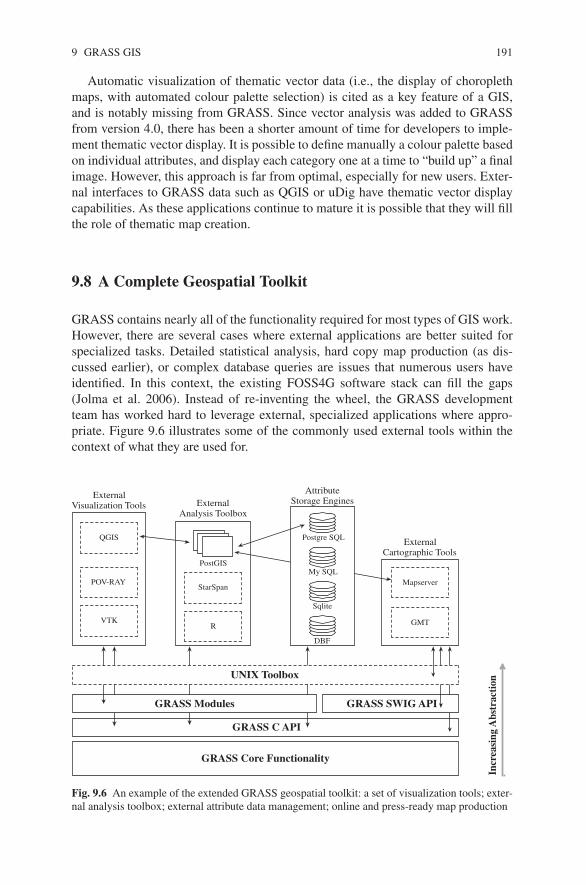
GRASS contains nearly all of the functionality required for most types of GIS work.However, there are several cases where external applications are better suited forspecialized tasks. Detailed statistical analysis, hard copy map production (as dis-cussed earlier), or complex database queries are issues that numerous users haveidentified. In this context, the existing FOSS4G software stack can fill the gaps(Jolma et al. 2006). Instead of re-inventing the wheel, the GRASS developmentteam has worked hard to leverage external, specialized applications where appro-priate. Figure 9.6 illustrates some of the commonly used external tools within thecontext of what they are used for.

QGIS

ExternalVisualization Tools

VTK

POV-RAY

GRASS Core Functionality

StarSpan

R

ExternalAnalysis Toolbox

PostGIS

Mapserver

GMT

ExternalCartographic Tools

GRASS C API

GRASS SWIG APIGRASS Modules

UNIX Toolbox

My SQL

AttributeStorage Engines

Postgre SQL

Sqlite

DBF

Incr

easi

ng A

bstr

acti

on

Fig. 9.6 An example of the extended GRASS geospatial toolkit: a set of visualization tools; exter-nal analysis toolbox; external attribute data management; online and press-ready map production

192 M. Neteler et al.

These applications, when coupled with the core GRASS modules through bothloose (i.e., using intermediate files of commonly structured text or binary data totransfer information between applications) and tight (i.e., using program APIs andinter-process messaging to pass data between applications) coupling, can fulfill eventhe most demanding spatial analysis needs.

9.8.1 External Attribute Storage

The default storage engine for tabular, or attribute, data is the well-known xBASE(DBF) table format. The GRASS database abstraction routines provide a simpleSQL interface to the xBASE files. However, advanced SQL constructs and datatypes are not supported. These are, however, available through the use of industry-strength RDBMS such as SQLite, PostgreSQL, or MySQL as the repository forattribute data. GRASS provides “tight integration” to these applications, allowingthe user to switch freely between RDBMS backends with the db.connect module.

9.8.2 Graphical User Interfaces

Quantum GIS (QGIS, http://qgis.org) has emerged as a favourite FOSS4G 2D visu-alization environment for GRASS users, providing a modern user interface and mapelement symbology editor. The current version of QGIS contains a graphical inter-face to most GRASS tools, a graphical data catalogue, and a native vector digitizer.Javagrass (http://www.jgrass.org), a client-server implementation, is an alternativeuser interface which includes 3D visualization. It comes with special focus on hy-drological and geomophological analysis. The fusion with the uDig software projectis currently ongoing, adding 3D visualization and further GIS analytical capabilitiesto uDig.

9.8.3 Visualization

The built-in visualization module NVIZ is very efficient and powerful. It supportsraster and vector data including 3D and raster volumes. Flight-simulator mode, high-resolution output, and custom animations complete the suite.

The Persistance of Vision Raytracer (POV-Ray, http://www.povray.org/) hasbeen used for over a decade by professional graphic designers to render complex3D scenes, complete with realistic lighting and surface interaction. The modulesr.out.pov and v.out.pov convert GRASS raster and vector data types into a formatsuitable for inclusion in a POV-Ray scene file (Fig. 9.7(a)).

The Visualization Toolkit (VTK) has recently emerged as an exciting new wayto interact with GRASS raster, vector, and volume datasets. Paraview, an integrated

9 GRASS GIS 193

(a) (b)

Fig. 9.7 Examples of external applications, POV-Ray (a) and Paraview (b), commonly used tovisualize complex 2, 3, and 4 dimensional GRASS datasets

visualization application based on VTK, is a modern analogue to NVIZ and in itslatest version is implemented with the cross-platform Qt GUI toolkit. The modulesv.out.vtk, r.out.vtk, and r3.out.vtk are used to export GRASS raster, vector, and vol-ume datasets (Fig. 9.7(b)).

9.8.4 Statistical Analysis

While several modules within the core GRASS system can perform simple sta-tistical summaries or compute correlation coefficients, R (R Development CoreTeam 2006), the OS implementation of the “S” statistical language, is the FOSSplatform of choice for detailed statistical analysis. R has a long history of compati-bility with GRASS, and connecting the two is as simple as installing the necessarypackages in the R environment. The interface between GRASS and R has been un-der rapid development over the last two years, and the current implementation hassimplified the process significantly (Bivand 2007). R software is hosted at Source-Forge (http://r-spatial.sourceforge.net), and includes spgrass6 (the main R-GRASSinterface), sp (the basic spatial object classes), spGDAL (a wrapper for functions inthe rgdal package which interfaces to the GDAL library – see Chap. 5), and spmap-tools (an interface to the shapelib library – see Chap. 5).

Regional or “zonal” statistics can be calculated within GRASS using thev.rast.stats script, however Starspan (http://starspan.casil.ucdavis.edu/), a more ma-ture implementation of these functions written in C++, can be used instead. Starspanuses the GDAL library to read natively GRASS raster and vector data for the calcu-lation of zonal statistics. Results are saved in comma separated values (CSV) format,which can easily be read into R for statistical analysis or back into GRASS.

Several examples of descriptive, geo-statistical, and other standard functions in Rcan be found in the GRASS Wiki site (http://grass.osgeo.org/wiki, see also Figs. 9.8

194 M. Neteler et al.

1000 1200 1400 1600 1800

0.0

0.2

0.4

0.6

0.8

1.0

ECDF of Elevation Data

(a) (b)

Elevation (m)

Fn(

x)

metamorphic

transition

igneous

sandstone

limestone

shale

sandy shale

claysand

sand

1200

1400

1600

1800

Elevation (m)

Fig. 9.8 Simple exploratory statistics performed in R on elevation (a) and geology (b) raster data

distance

sem

ivariance

20000

40000

60000

80000

100000

2000 4000 6000 8000 10000

0 45

90

2000 4000 6000 8000 10000

20000

40000

60000

80000

100000

135

dx

dy

–5000

0

5000

–5000 0 5000

elev

0

20000

40000

60000

80000

100000

120000

140000

160000

(a) (b)

Fig. 9.9 An exploration of anisotropy with directional variograms (a) and a variogram map (b)

and 9.9). The examples used here are based on the “Spearfish” sample data location(South Dakota, USA, 103.86W, 44.49N), the classical GRASS sample data set.

9.8.5 Cartographic Tools

As noted earlier, simple maps can be printed with the help of QGIS as an inter-face, while several other options are available for more complex tasks. MapServer(Lime 1996 – see Chap. 4 of this book) is a common gateway interface (CGI)application targeted at the production of online maps. It functions as the primary

9 GRASS GIS 195

cartographic engine behind many popular online mapping applications. MapServercan directly read GRASS raster and vector data through the GDAL library, makingit possible to serve maps online immediately after they are produced without theneed for intermediate conversion. The expressive map description language used byto define symbology, coupled with features such as automated label placement andcollision detection make MapServer a powerful map making tool.

The GMT suite (http://gmt.soest.hawaii.edu/) consists of 60 specialized mapmaking commands which output to publication-quality PostScript format. WithGMT in hand, it is possible to fill the gap in hard copy map production whichhas troubled GRASS users for years. Several attempts have been made at integrat-ing GRASS and GMT (Beaudette 2007). However, most are based on the “looselycoupled” approach of using intermediate files. Recent developments in the GDAL li-brary, maturation of the Python/SWIG API, and planned Python integration in GMT5.0 suggest that a more generalized and coherent fusion of GRASS and GMT willbe possible in the near future.

9.9 The GRASS is Growing: Reaching the World

The source code accessibility and the modular character of GRASS render the soft-ware an ideal platform for further development. The core system with its analyticalcapabilities can be accessed externally using several programmable approaches inorder to build graphical user interfaces upon it, or to use GRASS as the backbonefor external applications.

9.9.1 Making GRASS Accessible with a GUI

In place of a monolithic graphic interface to the GRASS modules, several small GUIsystems have emerged over the years. Initially based on the TclTk GUI frameworktcltkgrass, d.m and its successor gis.m have provided a simple interface to commonGIS analysis and visualization. These modules use a simple palette construct fordefining a list of commands like d.rast or d.vect, with common GUI constructs suchas buttons, check boxes, and forms for defining style elements. The GUI for NVIZ(the 3D interface to GRASS raster, vector, and volumetric data) and v.digit (theGRASS vector digitizer tool) were also built with the TclTk framework. TclTk haslong been used as a robust, multi-platform GUI toolbox. However, it is starting toshow its age.

The new GUI, wxGRASS, provides a modern-looking, compact layout of the coreGRASS functionality along with operating system-native graphical elements (alsoknown as widgets). Python/wxPython provides numerous GUI primitives (such ascolor pickers, combo box menus, etc.) which simplify the underlying code, andenable users to adjust display properties quickly. In addition, the conversion from

196 M. Neteler et al.

TclTK to the popular Python language opens development to a wide audience ofPython programmers. Object-oriented design, simple extensions of functionalitythough loadable modules, and advanced array handling are just some of the fea-tures Python has to offer. The wxGRASS interface contains several new and updatedfeatures. A built-in attribute management system with query support simplifies tablemanipulation operations. Improved type rendering and printing support also facili-tate rapid map production.

9.9.2 SWIG/Python Interface

The Simplified Wrapper and Interface Generator (SWIG-http://www.swig.org/) isa framework for connecting internal functions (i.e. GRASS C and C++ API) to anassortment of popular scripting languages such as TclTk, MATLAB, Perl, Python,PHP, JAVA etc. The SWIG compiler reduces the tedium of writing language-specificextensionmodules by automating the entire process. A functional prototype GRASS-SWIGinterface was recently implemented. The GRASS-SWIG interface opens the com-plex GRASS core-API functionality to developers who may be more proficientin, or prefer the flexibility of, different scripting languages. In addition, as thenumber of SWIG-enabled projects increases it will become possible to create acustom meta-API (in Python, for example) which bridges multiple distinct appli-cations. More information on the GRASS-SWIG interface can be found on theGRASS Wiki.

9.9.3 GRASS: A GIS Backbone for Web Applications

Web-based spatial services are developed for many applications. In particular, op-portunities for integrating data from various Spatial Data Infrastructure (SDI) por-tals into Internet-based services have grown. Interoperability and standardization areaccomplished by following standards such as those set by the OGC for spatial dataand related information technologies. While internally data storage and process-ing may differ from proposed OGC standards, all recent FOSS4G systems providedata exchange interfaces consistent with industrial standards. FOSS4G applicationscan either directly read GRASS raster and vector data through GDAL/OGR inter-operability, or, GRASS vector data can be stored in a PostGIS-compliant spatialdatabase, which is then linked to the application.

The Python Web Processing Service (PyWPS, http://pywps.wald.intevation.org)is a relatively new project started in spring 2006, which aims at implementing theOGC Web Processing Service (WPS) standard. A WPS can be configured to of-fer any sort of GIS functionality to clients across a network, including access topre-programmed calculations and/or computational models that operate on spatially

9 GRASS GIS 197

Fig. 9.10 Scheme of PyWPS (Python Web Processing Service)

referenced data. A WPS may offer calculations as simple as subtracting one set ofspatially referenced numbers from another (e.g., determining the difference in in-fluenza cases between two different seasons), or as complicated as a global climatechange model. The data required by the WPS can be delivered across a network, orbe available at the server.

PyWPS acts as a as translator between requests from a client and the workingtool (GRASS), installed on the server. In this way, the capabilities of GRASS areextended from a simple desktop application to a complete network-oriented system.Figure 9.10 illustrates the conceptual scheme of this approach.

The WPS standard is similar to other better known OGC standards, for ex-ample the Web Mapping Service (WMS) or Web Feature Service (WCS). It ac-cepts three types of requests, namely GetCapabilities, DescribeProcess andExecute. Each server offers several processes (tasks), which it is able to provide.Each process has defined inputs and outputs. Data inputs and outputs are Complex-Value (raster or vector maps or reference to them). Other inputs can be of type literalvalue or bounding box value. With GRASS, all possible tasks can be performed,which do not require direct interaction with the map display. With the combinationof WPS-clients (which can be a Web application in a Web browser, or plugin to adesktop GIS), a user does not have to install large GIS packages on his/her desktopas the application is running on a remote server.

9.10 The Future: GRASS in the FOSS4G Arena

Ongoing development will lead to GRASS Version 7 which will address severalimportant issues. The GRASS raster libraries need an overhaul in order to take ad-vantage of modern storage mechanisms such as tiling and caching. In preparation fornew (computational) challenges, parallelization of numerical operations will be ex-tended in order to support better calculations on computer grids and distributed sys-tems. Virtual linking of raster and vector data sources is planned, which will reducethe number of import operations for most projects. Improvements in the image pro-cessing library are directly linked to changes in the raster library. However, linking

198 M. Neteler et al.

development to the Open Source Security Information Management (OSSIM) APImight be a sensible way to avoid parallel development. Along with these changes,better support will be added for time series in GRASS, based on SQL constructs.

The vector processing modules are in need of transaction support. In particular, atechnology is required which would preserve geometry in the event of an incompleteor otherwise unexpected termination of an editing session. Furthermore, better useof spatial indexing should reduce the computational overhead required to build ormaintain topology during and after geometric operations. The net result of most ofthe planned changes will result in better response times, and will enable GRASS toserve better as an analytical backbone for Web GIS and Web Processing Services.

The 2007 and 2008 Google Summer of Code (SoC) program has sponsoredseveral GRASS-related projects including improved line generalization algorithms,least-cost path calculation based on global minima, a new module to compute least-cost paths in vector space (as opposed to the current raster-based approach) andothers. These projects address several long standing issues which have been raisedon the GRASS mailing list and feature-request system. The SoC program will bean important developer recruitment facilitator, and future projects are already beingplanned.

From the end user’s perspective, GRASS is one of the few complete analyticalFOSS4G projects available. It has evolved from its humble origins as a land man-agement tool for military installations into one of the most comprehensive, generalpurpose GIS available. Support for environmental applications has been an integralpart of its twenty plus years of development. Environmental and social data fromvarious sources can be easily integrated into a GRASS project and this makes thesoftware an attractive option to satisfy a wide range of application needs.

References

Beaudette DE (2007) Producing press-ready maps with GRASS and GMT. J Open Source Geospa-tial Foundation 1:29–35

Bivand R (2007) Using the R-GRASS interface. J Open Source Geospatial Foundation 1:36–38Blazek R (2005) Introducing the linear reference system in GRASS. Int J Geoinformatics

1(3):95–100Bouktif S, Antoniol G, Merlo E, Neteler M (2006) A novel approach to optimize clone refactoring

activity. In GECCO ’06: Proceedings of the 8th annual conference on Genetic and evolutionarycomputation, ACM Press, New York, USA, pp 1885–1892

Brovelli M, Cannata M, Longoni U (2004) LIDAR data filtering and DTM interpolation withinGRASS. Trans GIS 8(2):155–174

Hofierka J, Mitasova H, Neteler M (2008) Terrain parameterization in GRASS. In: Hengl T, ReuterH (eds) Geomorphometry: concepts, software, applications, Developments in Soil Science, Vol.33, Elsevier, Amsterdam pp. 387–410.

Issaks EH, Srivastava RM (1989) An introduction to applied geostatistics. Oxford University Press,England

Jenson JR (2000) Remote sensing of the environment: and earth science perspective. Prentice Hall,New Jersey

9 GRASS GIS 199

Jolma A, Ames D, Horning N, Neteler M, Racicot A, Sutton T (2006) Free and open source geospa-tial tools for environmental modeling and management. In: Voinov A (ed) Proc. iEMSs 2006,Session W13, July 9–13, 2006, Burlington, Vermont, USA

Lime S (1996) UMN MapServer, University of Minnesota, USA, [Computer Program]. Available:http://mapserver.gis.umn.edu

Lo CP, Yeung AKW (2006) Concepts and techniques of geographic information systems. PrenticeHall, New Jersey

Mitasova H, Hofierka J (1993) Interpolation by regularized spline with tension: II. Application toterrain modeling and surface geometry analysis. Math Geol 25(6):657–669

Mitasova H, Mitas L (1993) Interpolation by regularized spline with tension: I. Theory and imple-mentation. Math Geol 25(6):641–655

Neteler M, Grasso D, Michelazzi I, Miori L, Merler S, Furlanello C (2005) An integrated toolboxfor image registration, fusion and classification. Int J Geoinformatics 1:51–61

Neteler M, Mitasova H (2008) Open source GIS: A GRASS GIS approach. 3 edn. Springer,New York

R Development Core Team (2006) R: A language and environment for statistical computing.R foundation for statistical computing, Vienna, Austria. ISBN 3-900051-07-0

Rizzoli A, Neteler M, Rosa R, Versini W, Cristofolini A, Bregoli M, Buckley A, Gould E (2007)Early detection of TBEv spatial distribution and activity in the Province of Trento assessedusing serological and remotely-sensed climatic data. Geospatial Health 1(2):169–176