CHAPTER 9 OUT-OF-CONTROL PATTERNS

Sections Introduction Between- and Within-Group Variation Types of Control Chart Patterns Out-of-Control Patterns and the Rules of Thumb Summary Exercises References Chapter Objectives

To define and illustrate two types of special variation: periodic (between group) variation and persistent (within group) variation

To distinguish between within group variation and common variation

To discuss and illustrate characteristic control chart patterns, enabling the identification of special variation

9.1 Introduction

We have seen that a control chart identifies special (or assignable or exogenous) causes of variation. If special causes of variation are resolved, then the process is stable with only common causes of variation (random noise). In this chapter, we present different control chart patterns which indicate the presence of special causes of variation.

9.2 Between- and Within-Group Variation

Special (or assignable or exogenous) causes of variation can be classified into two types: periodic disturbances and persistent disturbances. 9.2.1 Periodic Disturbances Periodic disturbances create special causes of variation that intermittently affect a process. The intermittent nature of these causes tends to affect sampled observations separated in time and, hence, in different subgroups. This is called between-group variation. The effect of between-group variation is to create control chart patterns in which subgroup statistics are beyond the control limits; in other words, it yields control limits which are too narrow for the subgroup statistics. Examples of causes of variation that could generate between-group variation include:

Chaotic (unstable) functioning of automatic control devices.

Operator carelessness in setting up machine runs.

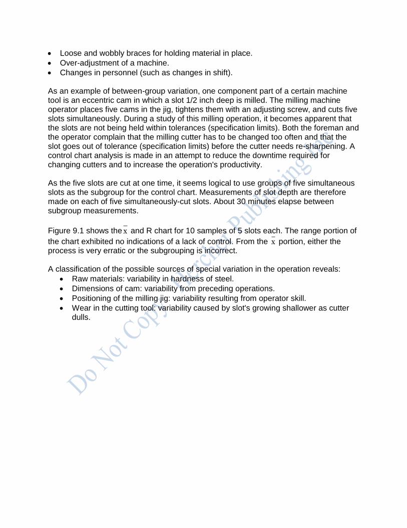
Loose and wobbly braces for holding material in place.

Over-adjustment of a machine.

Changes in personnel (such as changes in shift). As an example of between-group variation, one component part of a certain machine tool is an eccentric cam in which a slot 1/2 inch deep is milled. The milling machine operator places five cams in the jig, tightens them with an adjusting screw, and cuts five slots simultaneously. During a study of this milling operation, it becomes apparent that the slots are not being held within tolerances (specification limits). Both the foreman and the operator complain that the milling cutter has to be changed too often and that the slot goes out of tolerance (specification limits) before the cutter needs re-sharpening. A control chart analysis is made in an attempt to reduce the downtime required for changing cutters and to increase the operation's productivity. As the five slots are cut at one time, it seems logical to use groups of five simultaneous slots as the subgroup for the control chart. Measurements of slot depth are therefore made on each of five simultaneously-cut slots. About 30 minutes elapse between subgroup measurements.

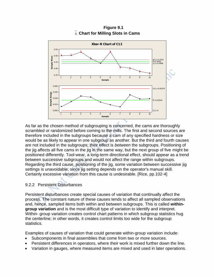
Figure 9.1 shows the x and R chart for 10 samples of 5 slots each. The range portion of

the chart exhibited no indications of a lack of control. From the x portion, either the process is very erratic or the subgrouping is incorrect. A classification of the possible sources of special variation in the operation reveals:

Raw materials: variability in hardness of steel.

Dimensions of cam: variability from preceding operations.

Positioning of the milling jig: variability resulting from operator skill.

Wear in the cutting tool: variability caused by slot's growing shallower as cutter dulls.

Figure 9.1

x Chart for Milling Slots in Cams

10987654321

0.55

0.50

0.45

0.40

0.35

Sample

Sa

mp

le M

ea

n

__X=0.4555UC L=0.4701

LC L=0.4408

10987654321

0.060

0.045

0.030

0.015

0.000

Sample

Sa

mp

le R

an

ge

_R=0.02544

UC L=0.05379

LC L=0

1

1

11

1

1

1

11

Xbar-R Chart of C12

As far as the chosen method of subgrouping is concerned, the cams are thoroughly scrambled or randomized before coming to the mills. The first and second sources are therefore included in the subgroups because a cam of any specified hardness or size would be as likely to appear in one subgroup as another. But the third and fourth causes are not included in the subgroups; their effect is between the subgroups. Positioning of the jig affects all five cams in the jig in the same way, but the next group of five might be positioned differently. Tool-wear, a long-term directional effect, should appear as a trend between successive subgroups and would not affect the range within subgroups. Regarding the third cause, positioning of the jig, some variation between successive jig settings is unavoidable, since jig setting depends on the operator's manual skill. Certainly excessive variation from this cause is undesirable. [Rice, pp.102-4]

9.2.2 Persistent Disturbances Persistent disturbances create special causes of variation that continually affect the process. The constant nature of these causes tends to affect all sampled observations and, hence, sampled items both within and between subgroups. This is called within-group variation and is the most difficult type of variation to identify and interpret. Within- group variation creates control chart patterns in which subgroup statistics hug the centerline; in other words, it creates control limits too wide for the subgroup statistics. Examples of causes of variation that could generate within-group variation include:

Subcomponents in final assemblies that come from two or more sources.

Persistent differences in operators, where their work is mixed further down the line.

Variation in gauges, where measured items are mixed and used in later operations.

As an extreme example of within-group variation, shafts are cut to length by two machines: A and B. Each machine cuts 50 percent of all shafts, and each machine accomplishes its task in approximately the same amount of time. Machine A's shafts are mostly good, but machine B's shafts are mostly defective. Figure 9.2 presents a schematic of machines A and B.

Figure 9.2

Work Flow of Cut-to-Length Operation

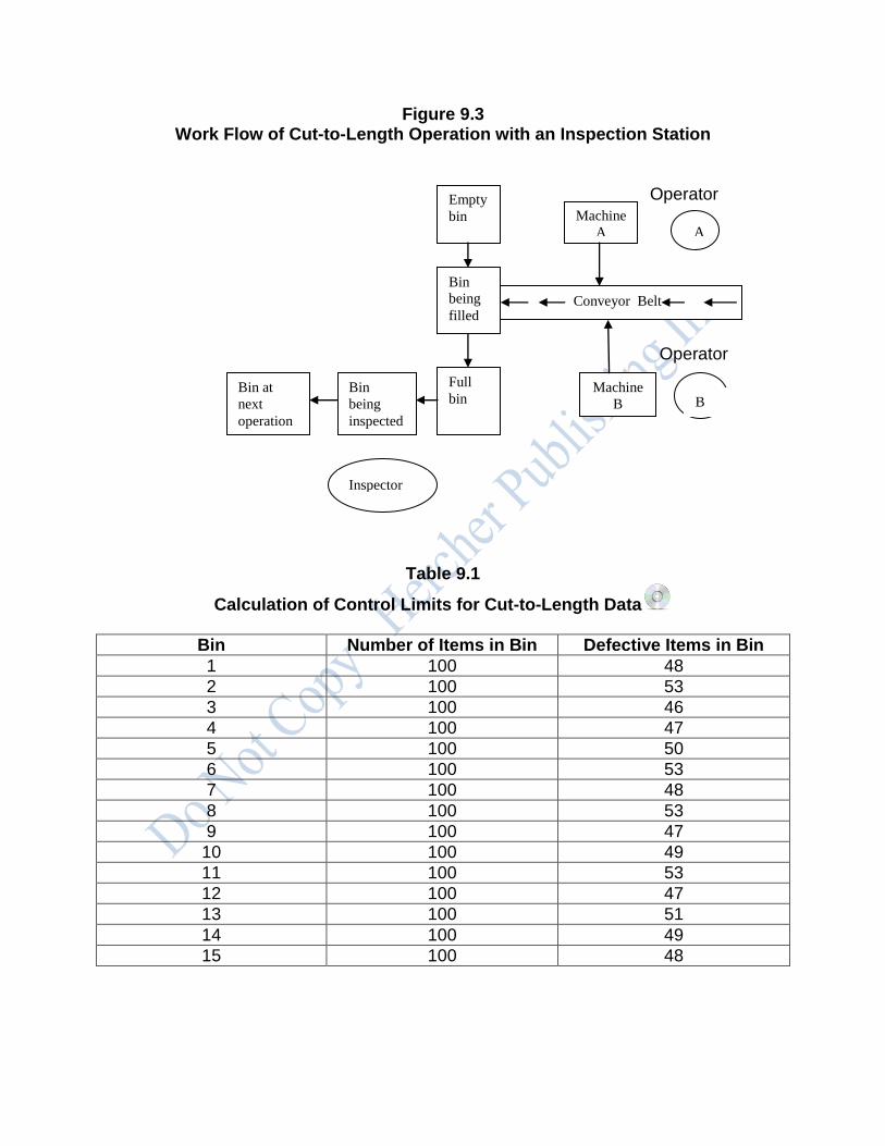
Operator Operator As shafts are finished, they are placed on the conveyor belt and fall into a bin, which can hold 100 shafts. Once a bin is filled, a new one is placed at the end of the conveyor to take its place. Consequently, approximately 50 percent of the shafts in any bin are from machine A; the other 50 percent are from machine B. The bins are then taken to the next operation. Employees at this next operation have started to complain about defective shafts. An inspection station is set up, as shown in Figure 9.3, and control chart limits are calculated from 100 percent inspection of every

20th bin, as shown in Table 9.1, from the data in LENGTH.

Empty

bin

Machine A

Conveyor belt

Bin

being

filled

Machine B

A

B

Full

bin

Bin at

next

operation

Figure 9.3 Work Flow of Cut-to-Length Operation with an Inspection Station

Operator Operator

Table 9.1

Calculation of Control Limits for Cut-to-Length Data

Bin Number of Items in Bin Defective Items in Bin

1 100 48

2 100 53

3 100 46

4 100 47

5 100 50

6 100 53

7 100 48

8 100 53

9 100 47

10 100 49

11 100 53

12 100 47

13 100 51

14 100 49

15 100 48

Empty

bin Machine

A A

Bin

being

filled Conveyor Belt

Full

bin Machine

B B Bin

being

inspected

Inspector

Bin at

next

operation

.3447 3).4947 (.505

3 -.4947 LCL

.6447 3).4947 (.505

3 .4947 UCL

04947 p

100

100

Figure 9.4 Minitab Control Chart for Cut-to-Length Data

151413121110987654321

0.65

0.60

0.55

0.50

0.45

0.40

0.35

0.30

Sample

Pro

po

rtio

n _P=0.4947

UCL=0.6447

LCL=0.3447

P Chart for Defectives

An examination of the control chart in Figure 9.4 shows that the fraction defective hugs the centerline. Recall that one would expect approximately two-thirds of all subgroup fractions to fall within one standard error of the mean; in this case, 100 percent fall in this region. Stated another way, it is extremely unlikely that a run of 13 or more points (in this case, 15) in a row would all fall within a one-sigma band on either side of the mean. The process is unusually “quiet”. A novice to control chart interpretation might say that this process exhibits a large degree of stability and predictability, although at a very high defect rate; this is erroneous. The shaft-cutting process is plagued by within-group variation. Each bin is made up of approximately 50 percent defective and 50 percent good shafts, resulting in large within-group variation and small between-group variation. As Figure 9.4 shows, this generates control limits too wide for the subgroup statistics. Three issues must be addressed in this shaft problem. First, the subgrouping should be made on a rational basis; that is, samples should be taken separately from machines A

and B. Second, the causes of machine B's defective output must be corrected. Last, both machines should be continually improved using statistical methods. 9.2.3 Distinguishing Within-Group Variation from Common Variation Both within-group special causes of variation and common causes of variation are persistent. However, the critical distinction is that within-group special sources of variation are external to the process, while common sources of variation are internal to the process. We need to realize that both between- and within-group special sources of variation must be resolved before the process can be considered stable. As we have discussed, stability is essential to process improvement.

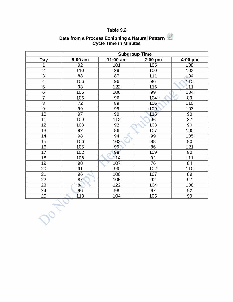
9.3 Types of Control Chart Patterns Identifiable control chart patterns can occur as a consequence of the presence of between- and/or within- group special causes of variations in a process. Fifteen characteristic patterns have been identified by Western Electric Company engineers [AT&T, 1956, pp. 161-80]: natural patterns; shift in level patterns (sudden shift in level, gradual shift in level, and trends); cycles; wild patterns (freaks and grouping/bunching); multi-universe patterns (mixtures: stable mixtures associated with systematic variables and with stratification; and unstable mixtures associated with freaks and with grouping/bunching); instability patterns; and relationship patterns (interaction and tendency of one chart to follow another). These patterns are useful because they can be compared with control charts in practice and used as diagnostic tools to detect special sources of variation. 9.3.1 Natural Patterns A natural pattern is one that does not exhibit points beyond the control limits, runs, or other nonrandom patterns and has most of the points near the centerline (approximately two-thirds of the points within a one-sigma band of the centerline). Natural processes are not disturbed by either between groups or within group special causes of variation. The process demonstrates a stable system of variation. Table 9.2 and Figure 9.5 illustrate a process with only common causes of variation for

the data in NATURAL. The data shows 25 days of cycles times in minutes with 4 data points per day drawn at 9:00am, 11:00am, 2:00pm, and 4:00pm. Please note the subgroups in table 9.2 are indicated by alternating patterns of bold and regular fonts.

Table 9.2

Data from a Process Exhibiting a Natural Pattern Cycle Time in Minutes

Subgroup Time

Day 9:00 am 11:00 am 2:00 pm 4:00 pm

1 92 101 105 108

2 110 89 100 102

3 88 87 111 104

4 106 96 96 115

5 93 122 116 111

6 106 106 99 104

7 106 96 104 89

8 72 89 106 110

9 99 99 109 103

10 97 99 115 90

11 109 112 96 87

12 103 92 103 90

13 92 86 107 100

14 98 94 99 105

15 106 103 88 90

16 105 99 86 121

17 102 98 109 90

18 106 114 92 111

19 98 107 76 84

20 91 99 102 110

21 96 100 107 89

22 87 105 92 97

23 84 122 104 108

24 96 98 97 92

25 113 104 105 99

Figure 9.5

Natural Pattern Control Chart

252321191715131197531

110

100

90

Sample

Sa

mp

le M

ea

n

__X=100.05

+3SL=114.83

-3SL=85.27

+2SL=109.90

-2SL=90.20

+1SL=104.98

-1SL=95.12

252321191715131197531

40

30

20

10

0

Sample

Sa

mp

le R

an

ge

_R=20.29

+3SL=46.28

-3SL=0

+2SL=37.61

-2SL=2.96

+1SL=28.95

-1SL=11.62

Xbar-R Chart of Cycle Time in Minutes

It is sometimes necessary to create external disturbances (special sources of variation) to a natural process to create improvements; for example, to move a process's average toward nominal or to reduce unit-to-unit variation in a process. The purpose of these external disturbances is to alter the process's basic structure. 9.3.2 Shift in Level Patterns There are three types of shift in level patterns: sudden shift in level, gradual shift in level, and trends. Sudden Shift in Level Patterns. A sudden shift in level pattern involves a sudden rise or fall in the level of data on a control chart. This is one of the most easily detectable control chart patterns.

Sudden shifts on x charts or on Individuals charts frequently result from a special source of variation which first shifts the process's average to a new level, but then has no further effect on the process. Sudden shifts on R charts can indicate the presence of some related variable affecting the process variability. For example, the addition of a new untrained worker to a trained and stable work force could increase the variability of output.

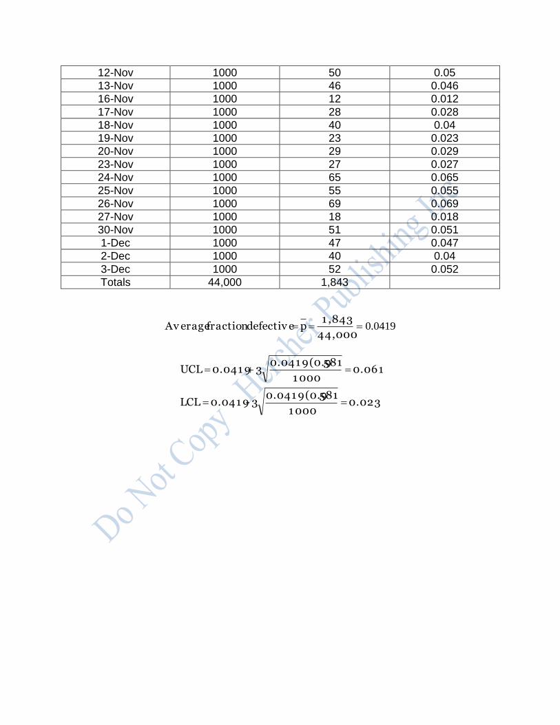
Sudden shifts on p charts can indicate such factors as a dramatic change in materials, methods, personnel, or operational definitions. If p is the proportion defective, then sudden shifts up indicate process degradation, while sudden shifts down indicate process improvement. To illustrate a sudden shift in level on a p chart, daily samples of the first 1,000 medium-sized ratchets produced are taken from a production process and tested for tight levers. The data appear in Table 9.3; they indicate many out-of-control points, as shown in the left panel of Figure 9.6. Some exogenous factor is apparently preventing consistent quality of work. A study of the assembly process soon reveals that the fixture used in welding the lever is poorly designed so that it is very difficult to obtain consistent welds.

Table 9.3

Ratchet Tight Lever Data

Date Sample Size Number Defectives Fraction Defective

3-Oct 1000 25 0.025

4-Oct 1000 18 0.018

5-Oct 1000 16 0.016

6-Oct 1000 20 0.02

7-Oct 1000 33 0.033

10-Oct 1000 65 0.065

11-Oct 1000 30 0.03

12-Oct 1000 92 0.092

13-Oct 1000 45 0.045

14-Oct 1000 26 0.026

17-Oct 1000 17 0.017

18-Oct 1000 30 0.03

19-Oct 1000 8 0.008

20-Oct 1000 74 0.074

21-Oct 1000 41 0.041

24-Oct 1000 29 0.029

25-Oct 1000 28 0.028

26-Oct 1000 35 0.035

27-Oct 1000 90 0.09

28-Oct 1000 51 0.051

2-Nov 1000 53 0.053

3-Nov 1000 67 0.067

4-Nov 1000 34 0.034

5-Nov 1000 55 0.055

6-Nov 1000 24 0.024

9-Nov 1000 60 0.06

10-Nov 1000 81 0.081

11-Nov 1000 44 0.044

12-Nov 1000 50 0.05

13-Nov 1000 46 0.046

16-Nov 1000 12 0.012

17-Nov 1000 28 0.028

18-Nov 1000 40 0.04

19-Nov 1000 23 0.023

20-Nov 1000 29 0.029

23-Nov 1000 27 0.027

24-Nov 1000 65 0.065

25-Nov 1000 55 0.055

26-Nov 1000 69 0.069

27-Nov 1000 18 0.018

30-Nov 1000 51 0.051

1-Dec 1000 47 0.047

2-Dec 1000 40 0.04

3-Dec 1000 52 0.052

Totals 44,000 1,843

0419.044,000

1 ,843 p defectiv e fraction Av erage

0.023 1 000

5810.041 9(0.93 - 0.041 9 LCL

0.061 1 000

5810.041 9(0.93 0.041 9 UCL

Figure 9.6

Minitab Sudden Shift in Level: p Chart for Old and New Ratchet Tight Lever Data

71645750433629221581

0.09

0.08

0.07

0.06

0.05

0.04

0.03

0.02

0.01

0.00

Sample

Pro

po

rtio

n

_P=0.0062

+3SL=0.0137

-3SL=0

+2SL=0.0112

-2SL=0.0012

+1SL=0.0087-1SL=0.0037

3-Oct 4-Dec

11

1

11

1

1

1

1

1

1

1

1

1

111

P Chart for Defectives

The fixture is redesigned and more data is collected, as shown in Table 9.4 and LEVER2. The redesigned fixture has eliminated most of the trouble and reduced the average percentage of tight levers from 4.2 percent to 0.6 percent. The old (left panel) and new (right panel) p charts in Figure 9.6 demonstrate a sudden shift in level.

Table 9.4

Redesigned Ratchet Tight Lever Data

Date Sample Size Number Defectives Fraction Defective

4-Dec 1000 8 0.008

5-Dec 1000 10 0.010

7-Dec 1000 2 0.002

8-Dec 1000 5 0.005

9-Dec 1000 10 0.010

10-Dec 1000 6 0.006

11-Dec 1000 7 0.007

14-Dec 1000 6 0.006

15-Dec 1000 3 0.003

16-Dec 1000 1 0.001

17-Dec 1000 2 0.002

18-Dec 1000 3 0.003

21-Dec 1000 0 0.000

22-Dec 1000 4 0.004

23-Dec 1000 7 0.007

24-Dec 1000 12 0.012

28-Dec 1000 9 0.009

29-Dec 1000 17 0.017

30-Dec 1000 15 0.015

31-Dec 1000 10 0.010

3-Jan 1000 8 0.008

4-Jan 1000 0 0.000

7-Jan 1000 6 0.006

8-Jan 1000 0 0.000

9-Jan 1000 3 0.003

10-Jan 1000 0 0.000

11-Jan 1000 1 0.001

14-Jan 1000 13 0.013

15-Jan 1000 12 0.012

4-Dec 1000 8 0.008

5-Dec 1000 10 0.010

7-Dec 1000 2 0.002

8-Dec 1000 5 0.005

9-Dec 1000 10 0.010

10-Dec 1000 6 0.006

11-Dec 1000 7 0.007

14-Dec 1000 6 0.006

15-Dec 1000 3 0.003

16-Dec 1000 1 0.001

17-Dec 1000 2 0.002

18-Dec 1000 3 0.003

21-Dec 1000 0 0.000

22-Dec 1000 4 0.004

23-Dec 1000 7 0.007

Totals 29,000 180

0.000 use .001 2- 1 000

938)0.0062(0.93 - 0.0062 LCL

1 000

938)0.0062(0.93 0.0062 UCL

29,000

1 80 p

0136.0

0062.0

Note in Figure 9.6 that the two points in the latter part of December are out of control as a result of a batch of faulty levers. Nevertheless, the 1.7 percent and 1.5 percent defective pieces found on these two days are fewer than were found most of the time on the old fixture. [Rice, pp. 70-74]

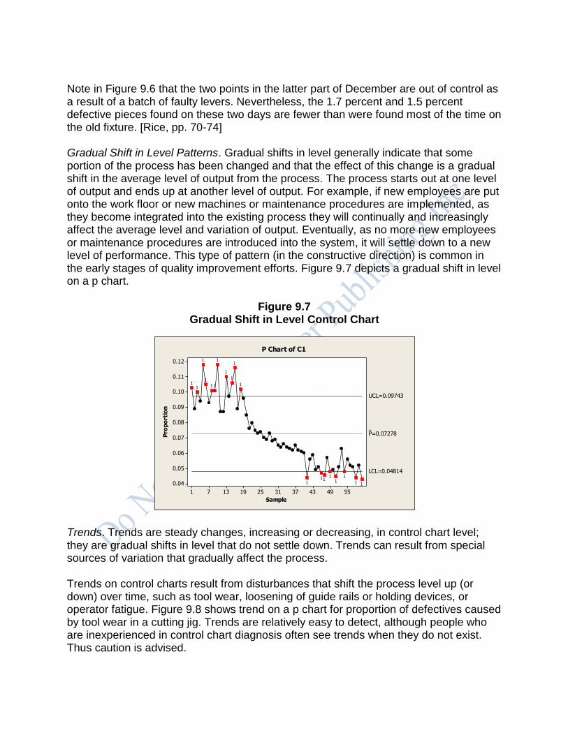
Gradual Shift in Level Patterns. Gradual shifts in level generally indicate that some portion of the process has been changed and that the effect of this change is a gradual shift in the average level of output from the process. The process starts out at one level of output and ends up at another level of output. For example, if new employees are put onto the work floor or new machines or maintenance procedures are implemented, as they become integrated into the existing process they will continually and increasingly affect the average level and variation of output. Eventually, as no more new employees or maintenance procedures are introduced into the system, it will settle down to a new level of performance. This type of pattern (in the constructive direction) is common in the early stages of quality improvement efforts. Figure 9.7 depicts a gradual shift in level on a p chart.

Figure 9.7

Gradual Shift in Level Control Chart

554943373125191371

0.12

0.11

0.10

0.09

0.08

0.07

0.06

0.05

0.04

Sample

Pro

po

rtio

n

_P=0.07278

UCL=0.09743

LCL=0.04814

11

11

111

1

1

1

1

1

1

11

1

1

11

P Chart of C1

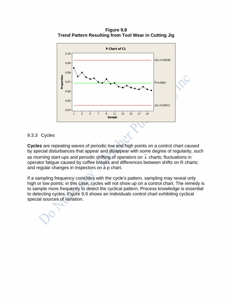
Trends. Trends are steady changes, increasing or decreasing, in control chart level; they are gradual shifts in level that do not settle down. Trends can result from special sources of variation that gradually affect the process. Trends on control charts result from disturbances that shift the process level up (or down) over time, such as tool wear, loosening of guide rails or holding devices, or operator fatigue. Figure 9.8 shows trend on a p chart for proportion of defectives caused by tool wear in a cutting jig. Trends are relatively easy to detect, although people who are inexperienced in control chart diagnosis often see trends when they do not exist. Thus caution is advised.

Figure 9.8 Trend Pattern Resulting from Tool Wear in Cutting Jig

191715131197531

0.10

0.09

0.08

0.07

0.06

0.05

0.04

Sample

Pro

po

rtio

n

_P=0.0692

UCL=0.09328

LCL=0.04512

P Chart of C1

9.3.3 Cycles Cycles are repeating waves of periodic low and high points on a control chart caused by special disturbances that appear and disappear with some degree of regularity, such

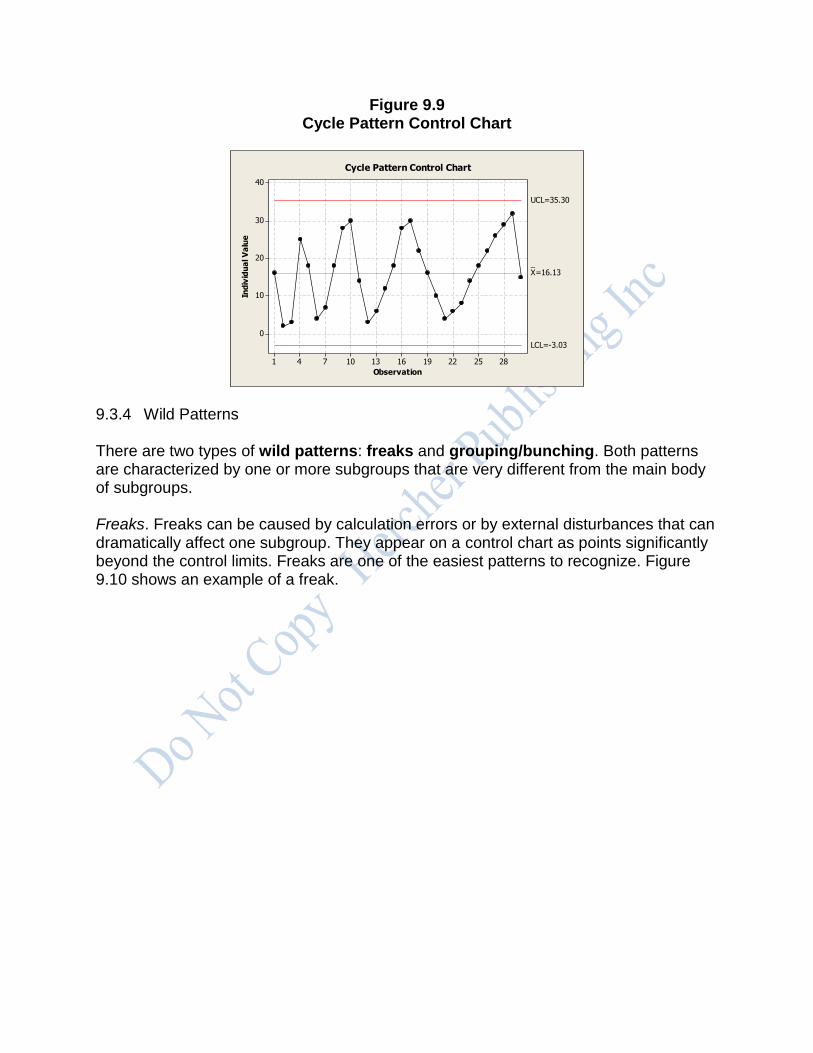
as morning start-ups and periodic shifting of operators on x charts; fluctuations in operator fatigue caused by coffee breaks and differences between shifts on R charts; and regular changes in inspectors on a p chart. If a sampling frequency coincides with the cycle's pattern, sampling may reveal only high or low points; in this case, cycles will not show up on a control chart. The remedy is to sample more frequently to detect the cyclical pattern. Process knowledge is essential to detecting cycles. Figure 9.9 shows an Individuals control chart exhibiting cyclical special sources of variation.

Figure 9.9 Cycle Pattern Control Chart

28252219161310741

40

30

20

10

0

Observation

Ind

ivid

ua

l V

alu

e

_X=16.13

UCL=35.30

LCL=-3.03

Cycle Pattern Control Chart

9.3.4 Wild Patterns There are two types of wild patterns: freaks and grouping/bunching. Both patterns are characterized by one or more subgroups that are very different from the main body of subgroups. Freaks. Freaks can be caused by calculation errors or by external disturbances that can dramatically affect one subgroup. They appear on a control chart as points significantly beyond the control limits. Freaks are one of the easiest patterns to recognize. Figure 9.10 shows an example of a freak.

Figure 9.10 Freak Pattern Control Chart

28252219161310741

45

40

35

30

25

20

15

10

Observation

Ind

ivid

ua

l V

alu

e

_X=21.3

UCL=32.76

LCL=9.84

Freak Pattern Control Chart

Grouping/Bunching. Grouping/bunching is caused by the introduction into a process of a new system of disturbances that affect a "group" or "bunch" of points that are close

together. Figure 9.11 illustrates grouping/bunching on an x and R chart. In this case the

grouping/bunching is a good special cause of variation and should be built into the process.

Figure 9.11 Grouping/Bunching Pattern Control Chart

9181716151413121111

120

100

80

Observation

In

div

idu

al

Va

lue

_X=101.13

UC L=126.89

LC L=75.37

9181716151413121111

30

20

10

0

Observation

Mo

vin

g R

an

ge

__MR=9.69

UC L=31.65

LC L=0

22222

2222

I-MR Chart of Waiting Time (Minutes)

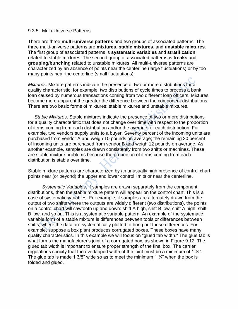
9.3.5 Multi-Universe Patterns There are three multi-universe patterns and two groups of associated patterns. The three multi-universe patterns are mixtures, stable mixtures, and unstable mixtures. The first group of associated patterns is systematic variables and stratification related to stable mixtures. The second group of associated patterns is freaks and grouping/bunching related to unstable mixtures. All multi-universe patterns are characterized by an absence of points near the centerline (large fluctuations) or by too many points near the centerline (small fluctuations). Mixtures. Mixture patterns indicate the presence of two or more distributions for a quality characteristic; for example, two distributions of cycle times to process a bank loan caused by numerous transactions coming from two different loan officers. Mixtures become more apparent the greater the difference between the component distributions. There are two basic forms of mixtures: stable mixtures and unstable mixtures. Stable Mixtures. Stable mixtures indicate the presence of two or more distributions for a quality characteristic that does not change over time with respect to the proportion of items coming from each distribution and/or the average for each distribution. For example, two vendors supply units to a buyer. Seventy percent of the incoming units are purchased from vendor A and weigh 10 pounds on average; the remaining 30 percent of incoming units are purchased from vendor B and weigh 12 pounds on average. As another example, samples are drawn consistently from two shifts or machines. These are stable mixture problems because the proportion of items coming from each distribution is stable over time. Stable mixture patterns are characterized by an unusually high presence of control chart points near (or beyond) the upper and lower control limits or near the centerline. Systematic Variables. If samples are drawn separately from the component distributions, then the stable mixture pattern will appear on the control chart. This is a case of systematic variables. For example, if samples are alternately drawn from the output of two shifts where the outputs are widely different (two distributions), the points on a control chart will sawtooth up and down: shift A high, shift B low, shift A high, shift B low, and so on. This is a systematic variable pattern. An example of the systematic variable form of a stable mixture is differences between tools or differences between shifts, where the data are systematically plotted to bring out these differences. For example, suppose a box plant produces corrugated boxes. These boxes have many quality characteristics. In this example we will focus on "glued tab width." The glue tab is what forms the manufacturer's joint of a corrugated box, as shown in Figure 9.12. The glued tab width is important to ensure proper strength of the final box. The carrier regulations specify that the overlapped width of the joint must be a minimum of 1 ¼”. The glue tab is made 1 3/8” wide so as to meet the minimum 1 ¼” when the box is folded and glued.

Figure 9.12

Glued Tab Width

Glued Tab Width 1 ¼” Minimum

Ten subgroups of the glued tab widths of four corrugated boxes were drawn from the

outputs of shift A and shift B. Figure 9.13 presents the data and x and R charts. The x chart shows a classic sawtooth pattern leading to the unusually high presence of control chart points beyond the control limits. The problem is the presence of a variable that systematically affects the process, in this case, shifts. The control charts in this example

should be separated into the x and R charts for shift A and shift B.

Figure 9.13 Systematic Variable-Stable Mixture Pattern Control Chart

10987654321

1.8

1.6

1.4

1.2

1.0

Sample

Sa

mp

le M

ea

n

__X=1.4138

UC L=1.6966

LC L=1.1310

10987654321

0.8

0.6

0.4

0.2

0.0

Sample

Sa

mp

le R

an

ge

_R=0.3882

UC L=0.8857

LC L=0

1

1

1

1

1

1

1

1

Xbar-R Chart of Glued Tab Width

Stratification. If samples are drawn from two or more distributions that have been combined, then the stable mixture pattern can create extremely small differences

among statistics in x , R, individuals, or p charts, resulting in an unusually high presence

of control chart points near the centerline. The small differences in x , R, individuals, or p charts are frequently interpreted by the novice control chart user as representing unusually good control; nothing could be further from the truth.

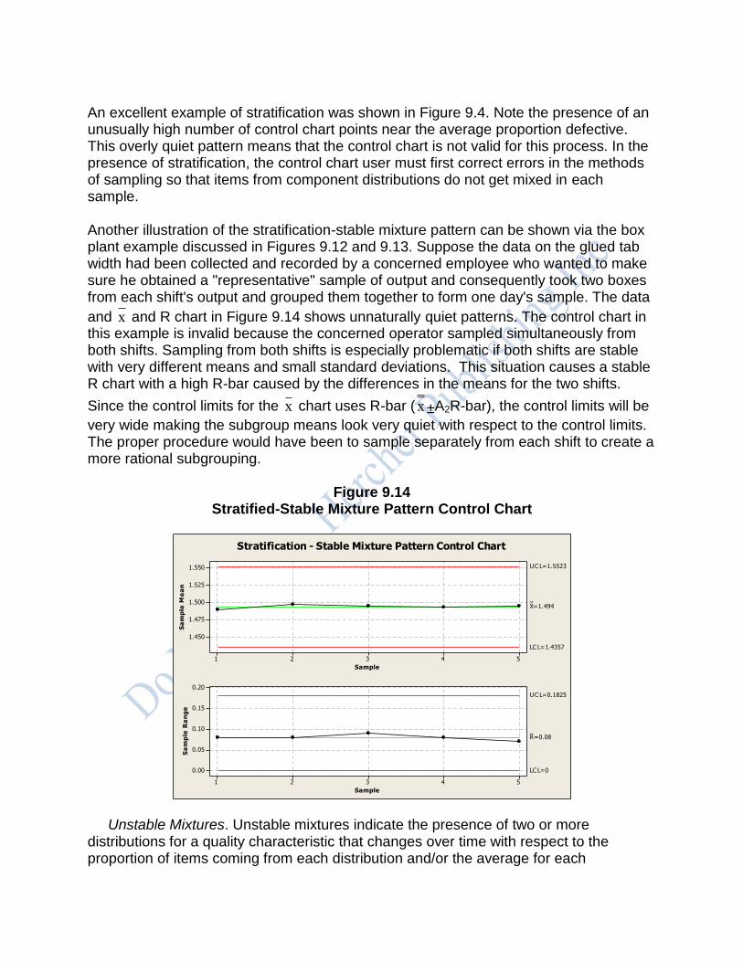
An excellent example of stratification was shown in Figure 9.4. Note the presence of an unusually high number of control chart points near the average proportion defective. This overly quiet pattern means that the control chart is not valid for this process. In the presence of stratification, the control chart user must first correct errors in the methods of sampling so that items from component distributions do not get mixed in each sample. Another illustration of the stratification-stable mixture pattern can be shown via the box plant example discussed in Figures 9.12 and 9.13. Suppose the data on the glued tab width had been collected and recorded by a concerned employee who wanted to make sure he obtained a "representative" sample of output and consequently took two boxes from each shift's output and grouped them together to form one day's sample. The data

and x and R chart in Figure 9.14 shows unnaturally quiet patterns. The control chart in this example is invalid because the concerned operator sampled simultaneously from both shifts. Sampling from both shifts is especially problematic if both shifts are stable with very different means and small standard deviations. This situation causes a stable R chart with a high R-bar caused by the differences in the means for the two shifts.

Since the control limits for the x chart uses R-bar ( x ±A2R-bar), the control limits will be

very wide making the subgroup means look very quiet with respect to the control limits. The proper procedure would have been to sample separately from each shift to create a more rational subgrouping.

Figure 9.14 Stratified-Stable Mixture Pattern Control Chart

54321

1.550

1.525

1.500

1.475

1.450

Sample

Sa

mp

le M

ea

n

__X=1.494

UC L=1.5523

LC L=1.4357

54321

0.20

0.15

0.10

0.05

0.00

Sample

Sa

mp

le R

an

ge

_R=0.08

UC L=0.1825

LC L=0

Stratification - Stable Mixture Pattern Control Chart

Unstable Mixtures. Unstable mixtures indicate the presence of two or more distributions for a quality characteristic that changes over time with respect to the proportion of items coming from each distribution and/or the average for each

distribution; for example, a buyer has two vendors for an item, and the proportion coming from each vendor and/or the quality characteristic averages for each vendor change over time. Figure 9.15 depicts an unstable mixture pattern.

Figure 9.15 Unstable Mixture Pattern Control Chart

V

332925211713951

40

30

20

10

0

Observation

Ind

ivid

ua

l V

alu

e

_X=16.31

UCL=38.72

LCL=-6.11

Unstable Mixture Pattern Control Chart

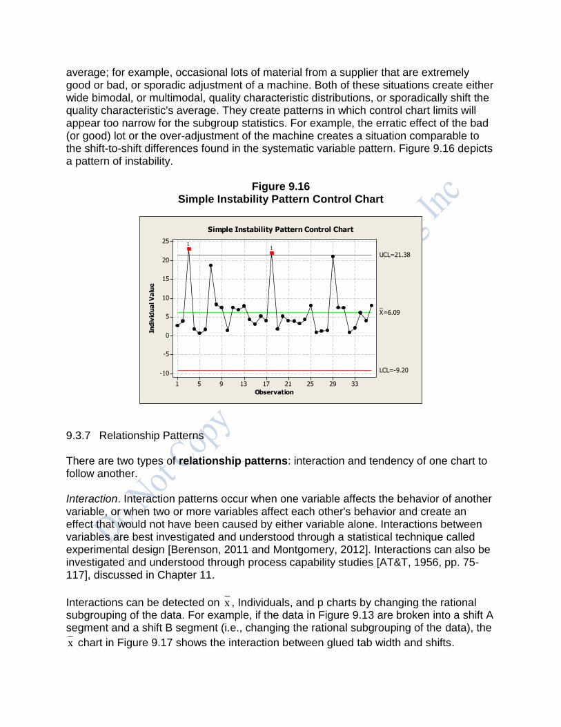
Freaks and Grouping/Bunching. The nature of an unstable mixture pattern implies that the multiple component distributions that make up the distribution of a quality characteristic are sporadically affected by special disturbances. This will cause a systematic variable effect, but one which will occur unevenly, generating an unusually large number of control chart points near or beyond the control limits. However, those points will be in groups or bunches, depending on the juxtaposition of the various component quality characteristic distributions. This pattern could also result in freaks. 9.3.6 Instability Patterns Erratic points on a control chart exhibiting large swings up and down characterize a pattern called instability. Instability is a possible result of special variation so that the control limits appear too narrow for the control chart. Instability is characterized by large, erratic fluctuations in subgroup statistics and is frequently associated with unstable mixtures. Instability is caused either by one special disturbance that can sporadically affect the average or variability of a process, or by two or more special disturbances, each of which can affect the average and/or variability of a process. These disturbances interact with each other and create complex process disturbances. Simple instability occurs when one special disturbance creates a wide, bimodal, or multimodal distribution in a quality characteristic or sporadically shifts the process

average; for example, occasional lots of material from a supplier that are extremely good or bad, or sporadic adjustment of a machine. Both of these situations create either wide bimodal, or multimodal, quality characteristic distributions, or sporadically shift the quality characteristic's average. They create patterns in which control chart limits will appear too narrow for the subgroup statistics. For example, the erratic effect of the bad (or good) lot or the over-adjustment of the machine creates a situation comparable to the shift-to-shift differences found in the systematic variable pattern. Figure 9.16 depicts a pattern of instability.

Figure 9.16

Simple Instability Pattern Control Chart

332925211713951

25

20

15

10

5

0

-5

-10

Observation

Ind

ivid

ua

l V

alu

e

_X=6.09

UCL=21.38

LCL=-9.20

11

Simple Instability Pattern Control Chart

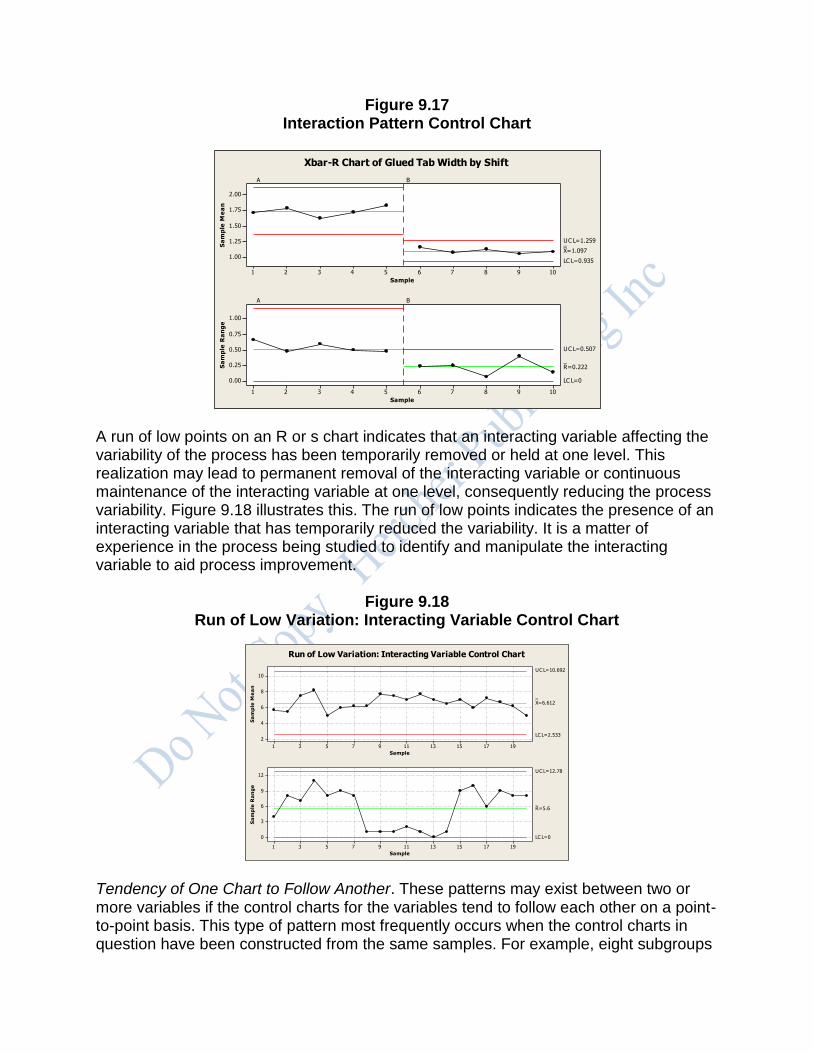
9.3.7 Relationship Patterns There are two types of relationship patterns: interaction and tendency of one chart to follow another. Interaction. Interaction patterns occur when one variable affects the behavior of another variable, or when two or more variables affect each other's behavior and create an effect that would not have been caused by either variable alone. Interactions between variables are best investigated and understood through a statistical technique called experimental design [Berenson, 2011 and Montgomery, 2012]. Interactions can also be investigated and understood through process capability studies [AT&T, 1956, pp. 75-117], discussed in Chapter 11.

Interactions can be detected on x , Individuals, and p charts by changing the rational subgrouping of the data. For example, if the data in Figure 9.13 are broken into a shift A segment and a shift B segment (i.e., changing the rational subgrouping of the data), the

x chart in Figure 9.17 shows the interaction between glued tab width and shifts.

Figure 9.17 Interaction Pattern Control Chart

10987654321

2.00

1.75

1.50

1.25

1.00

Sample

Sa

mp

le M

ea

n

__X=1.097

UC L=1.259

LC L=0.935

A B

10987654321

1.00

0.75

0.50

0.25

0.00

Sample

Sa

mp

le R

an

ge

_R=0.222

UC L=0.507

LC L=0

A B

Xbar-R Chart of Glued Tab Width by Shift

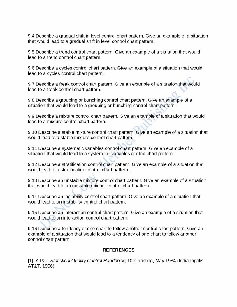
A run of low points on an R or s chart indicates that an interacting variable affecting the variability of the process has been temporarily removed or held at one level. This realization may lead to permanent removal of the interacting variable or continuous maintenance of the interacting variable at one level, consequently reducing the process variability. Figure 9.18 illustrates this. The run of low points indicates the presence of an interacting variable that has temporarily reduced the variability. It is a matter of experience in the process being studied to identify and manipulate the interacting variable to aid process improvement.

Figure 9.18 Run of Low Variation: Interacting Variable Control Chart

191715131197531

10

8

6

4

2

Sample

Sa

mp

le M

ea

n

__X=6.612

UC L=10.692

LC L=2.533

191715131197531

12

9

6

3

0

Sample

Sa

mp

le R

an

ge

_R=5.6

UC L=12.78

LC L=0

Run of Low Variation: Interacting Variable Control Chart

Tendency of One Chart to Follow Another. These patterns may exist between two or more variables if the control charts for the variables tend to follow each other on a point-to-point basis. This type of pattern most frequently occurs when the control charts in question have been constructed from the same samples. For example, eight subgroups

of four items can be measured with respect to two different quality characteristics (X and Y), and each measurement plotted on its respective control chart. Figure 9.19 illustrates one chart following another.

Figure 9.19 One Chart Following another Pattern Control Chart

87654321

30

25

20

15

10

5

0

Observation

Ind

ivid

ua

l V

alu

e

_X=16.25

UCL=30.31

LCL=2.19

Variable X

87654321

20

15

10

5

0

-5

-10

Observation

Ind

ivid

ua

l V

alu

e

_X=6.25

UCL=20.31

LCL=-7.81

Variable Y

9.4 Out-of-Control Patterns and the Rules of Thumb Natural control chart patterns exhibit the following characteristics: 1. Rarely will a point exceed the control limits. 2. Most (but not all) points are near the centerline. 3. A few (but not too many) points are near the control limits. 4. There are no nonrandom patterns among the points. 5. There is neither very high nor very low variability among the points. If one (or more) of these conditions is absent in a control chart pattern, the pattern will appear unnatural, exhibiting one or more of the following characteristics: 1. Points located beyond the control limits.

2. Absence of points near the centerline. 3. Absence of points near the control limits. 4. Nonrandom patterns among the points. 5. Exceptionally high or low variability among the points. These characteristics are reflected in the seven rules for detecting out-of-control behavior discussed in Chapter 6. For example, a stratification pattern would exhibit the absence of points near the control limits (too many points near the centerline), indicated by Rule 7; a grouping/bunching pattern would exhibit the absence of points near the centerline (too many points near or beyond the control limits), indicated by Rules 1, 2, 3, and/or 6; a freak pattern would exhibit points beyond the control limits, indicated by Rule 1; a systematic variable pattern would exhibit an unusually small number of runs up and down (a sawtooth pattern, alternating high, low, high, low, high), indicated by Rule 6; and a gradual shift or trend pattern would exhibit an unusually long run of points up or down, indicated by Rules 4 and/or 5.

9.5 Summary

We began this chapter by explaining the different types of special variation in an analytic study: between-group variation and within-group variation. Between-group sources of variation are external sources of variation that affect a process periodically, while within-group sources of variation affect a process persistently. There are fifteen control chart patterns whose detection is helpful in understanding and eliminating special sources of variation in a process: natural, sudden shift in level, gradual shift in level, trends, cycles, freaks, grouping or bunching, mixtures, stable mixtures with systematic variables, stable mixtures with stratification, unstable mixtures with freaks, unstable mixtures with grouping or bunching, instability, interaction, and tendency of one chart to follow another. These are related to the rules of thumb presented in Chapter 6. In general, all rules must be applied cautiously in the context of the process being analyzed.

EXERCISES 9.1 a. Define special variation. b. Define common variation. c. Define the two types of special variation: between-group variation and within- group variation. Explain the difference between them and give examples of each. 9.2 Describe a natural control chart pattern. Give an example of a situation that would lead to a natural control chart pattern. 9.3 Describe a sudden shift in level control chart pattern. Give an example of a situation that would lead to a sudden shift in level control chart pattern.

9.4 Describe a gradual shift in level control chart pattern. Give an example of a situation that would lead to a gradual shift in level control chart pattern. 9.5 Describe a trend control chart pattern. Give an example of a situation that would lead to a trend control chart pattern. 9.6 Describe a cycles control chart pattern. Give an example of a situation that would lead to a cycles control chart pattern. 9.7 Describe a freak control chart pattern. Give an example of a situation that would lead to a freak control chart pattern. 9.8 Describe a grouping or bunching control chart pattern. Give an example of a situation that would lead to a grouping or bunching control chart pattern. 9.9 Describe a mixture control chart pattern. Give an example of a situation that would lead to a mixture control chart pattern. 9.10 Describe a stable mixture control chart pattern. Give an example of a situation that would lead to a stable mixture control chart pattern. 9.11 Describe a systematic variables control chart pattern. Give an example of a situation that would lead to a systematic variables control chart pattern. 9.12 Describe a stratification control chart pattern. Give an example of a situation that would lead to a stratification control chart pattern. 9.13 Describe an unstable mixture control chart pattern. Give an example of a situation that would lead to an unstable mixture control chart pattern. 9.14 Describe an instability control chart pattern. Give an example of a situation that would lead to an instability control chart pattern. 9.15 Describe an interaction control chart pattern. Give an example of a situation that would lead to an interaction control chart pattern. 9.16 Describe a tendency of one chart to follow another control chart pattern. Give an example of a situation that would lead to a tendency of one chart to follow another control chart pattern.

REFERENCES [1] AT&T, Statistical Quality Control Handbook, 10th printing, May 1984 (Indianapolis: AT&T, 1956).

[2] M. Berenson, D. Levine, and T. Krehbiel, Basic Business Statistics: Concepts and Applications, 12th Edition (Upper Saddle River, NJ: Pearson, 2011). [3] D.M. Montgomery, Design and Analysis of Experiments, 8th Edition (New York: John Wiley, 2012). [4] William B. Rice, Control Charts in Factory Management (New York: John Wiley & Sons, 1947)