Chapter II. Controlling Cars on a Bridge

Chapter II. Controlling Cars on a Bridge

1 Introduction

The intent of this chapter is to introduce a complete example of a small system development. During thisdevelopment, you will be made aware of the systematic approach we are using: it consists in developinga series of more and more accurate models of the system we want to construct. This technique is calledrefinement. The reason for building consecutive models is that a unique one would be far too complicatedto reason about. Note that each model does not represent the programming of our system using a highlevel programming language, it rather formalizes what an external observer of this system could perceiveof it.

Each model will be analyzed and proved, thus enabling us to establish that it is correct relative to anumber of criteria. As a result, when the last model will be finished, we shall be able to say that thismodel is correct by construction. Moreover, this model will be so close to a final implementation that itwill be very easy to transform it into a genuine program.

The correctness criteria alluded to above will be made completely clear and systematic by giving anumber of proof obligation rules which will be applied on our models. After applying such rules, weshall have to prove formally a number of statements. To this end, we shall also give a reminder of theclassical rules of inference of the sequent calculus. Such rules concern propositional logic, equality, andbasic arithmetic. The idea here is to give the reader the possibility to manually prove the statements asgiven by the proof obligation rules. Clearly, such proofs could easily be discharged by a theorem prover,but we feel that it is important at this stage for the reader to exercise himself before using an automatictheorem prover. Notice that we do not claim that a theorem prover would perform these proofs the way itis proposed here: quite often, a tool does not work like a human being does.

This chapter is organized as follows. Section 2 contains the requirement document of the system wewould like to develop: for this, we shall use the principles we have explained in the previous chapter.Section 3 explains our refinement strategy: it essentially assigns the various requirements to the variousdevelopment steps. The four remaining sections are devoted to the development of the initial models andthat of the three subsequent refinements.

2 Requirements Document

The system we are going to build is a piece of software, called the controller, connected to some equip-ment, called the environment. There are thus two kinds of requirements: those concerned with the func-tionalities of the controller labeled FUN, and those concerned with the environment labeled ENV.

Note that the model we are going to build is a closed model comprising the controller as well asits environment. The reason is that we want to define with great care the assumptions we are makingconcerning the environment. In other words, the controller we shall build eventually will be correct aslong as these assumptions are fulfilled by the environment: outside these assumptions, the controller isnot guaranteed to perform correctly. We shall come back to this in section 7.

Let us now turn our attention to the requirements of this system. The main function of this system is tocontrol cars on a narrow bridge. This bridge is supposed to link the mainland to a small island.

The system is controlling cars on a bridge connecting the mainland to an island FUN-1

1

This system is equipped with two traffic lights.

The system is equipped with two traffic lights with two colors: green and red ENV-1

One of the traffic lights is situated on the mainland and the other one on the island. Both are close to thebridge.

The traffic lights control the entrance to the bridge at both ends of it ENV-2

Drivers are supposed to obey the traffic lights by not passing when a traffic light is red.

Cars are not supposed to pass on a red traffic light, only on a green one ENV-3

There are also some car sensors situated at both ends of the bridge.

The system is equipped with four sensors with two states: on or off ENV-4

These sensors are supposed to detect the presence of cars intending to enter or leave the bridge. There arefour such sensors. Two of them are situated on the bridge and the other two are situated on the mainlandand in the island respectively.

The sensors are used to detect the presence of a car entering or leavingthe bridge: "on" means that a car is willing to enter the bridge or to leave it ENV-5

The pieces of equipment which have been described are illustrated Fig. 1.The system has two main addi-tional constraints: the number of cars on the bridge and island is limited

The number of cars on bridge and island is limited FUN-2

and the bridge is one-way.

The bridge is one-way or the other, not both at the same time FUN-3

2

BridgeIsland Mainland

traffic lightsensor

Fig. 1. The Bridge Control Equipment

3 Refinement Strategy

Before engaging in the development of such a system, it is profitable to clearly identify what our designstrategy will be. This is done by listing the order in which we are going to take account of the variousrequirements we proposed in the requirement document of the previous section. Here is our strategy:

– We start with a very simple model allowing us to take account of requirement FUN-2 concerned withthe maximum number of cars on the island and the bridge (section 4)

– Then the bridge is introduced into the picture, and we thus take account of requirement FUN-3 tellingus that the bridge is one way or the other (section 5).

– In the next refinement, we introduce the traffic lights. This corresponds to requirements ENV-1, ENV-2, and ENV-3 (section 6).

– In the last refinement, we introduce the various sensors corresponding to requirements ENV-4 andENV-5 (section 7). In this refinement, we shall also introduce eventually the architecture of our closedmodel made of the controller, the environment, and the communication channels between the two.

You may have noticed that we have not been speaking of requirement FUN-1 telling us what the mainfunction of this system is. This is simply because it is fairly general. It is in fact taken care of at eachdevelopment step.

4 Initial Model: Limiting the Number of Cars

4.1 Introduction

The first model we are going to construct is very simple. We do not consider at all the various piecesof equipment, namely the traffic lights and sensors, they will be introduced in subsequent refinements.Likewise, we do not even consider the bridge, only a compound made of the bridge and the island together.

This is a very frequent approach to be taken. We start to build a model which is far more abstract thanthe final system we want to construct. The idea is to take account initially of very few constraints only.

3

This is because we want to be able to reason about this system in a simple way, considering in turn eachrequirement.

As a useful analogy, we suppose to observe the situation from very high in the sky. Although we cannotsee the bridge, we suppose however that we can “see” the cars on the island-bridge compound and observethe two transitions, ML_out and ML_in, corresponding to cars entering and leaving the island-bridgecompound. All this is illustrated on Fig. 2.

ML_out

ML_in

Islandand

BridgeMainland

Fig. 2. The Mainland and the Island-Bridge

Our first task is to formalize the state of this simple version of our system (section 4.2). We shall thenformalize the two events we can observe (section 4.3).

4.2 Formalizing the State

The state of our model is made up of two parts: the static part and the dynamic part. The static partcontains the definition and axioms associated with some constants, whereas the dynamic part contains thevariables which are modified as the system evolves. The static part is also called the context of our model.

The context of our first model is very simple. It contains a single constant d, which is a natural numberdenoting the maximum number of cars allowed to be on the island-bridge compound at the same time.The constant d has a simple axiom: it is a natural number. As can be seen below, we have given this axiomthe name axm0_1:

constant: d axm0_1: d ∈ N

The dynamic part is made up of a single variable n, which denotes the actual number of cars in theisland-bridge compound at a given moment. This is simply written as shown in the following boxes:

variable: ninv0_1: n ∈ N

inv0_2: n ≤ d

4

Variable n is defined by means of two conditions which are called the invariants. They are namedinv0_1 and inv0_2. The reason to call them invariants is straightforward: despite the changes over time inthe value of n, these conditions remain always true. Invariant inv0_1 says that n is a natural number. Andthe first basic requirement of our system, namely FUN-2, is taken into account at this stage by statingin inv0_2 that the number n of cars in the compound is always smaller than or equal to the maximumnumber d.

The labels axm0_1, inv0_1, and inv0_2 we have used above are chosen in a systematic fashion. Theprefix axm stands for the axiom of the constant d whereas the prefix inv stands for the invariant of thevariable n. The 0, as in axm0_1 or inv0_2, stands for the fact that these conditions are introduced in theinitial model. Subsequent models will be the first refinement, the second refinement, and so on. They willbe numbered 1, 2, etc. Finally, the second number, as 2 in inv0_2, is a simple serial number. In the sequel,we shall use such a systematic labeling scheme for naming our state conditions. Sometimes, but rarely,we shall change the prefixes axm and inv for others. We found this naming scheme convenient, but, ofcourse, any other naming scheme can be used provided it is systematic.

4.3 Formalizing the Events

At this stage, we can observe two transitions, which we shall call events in the sequel. They correspondto cars entering the island-bridge compound or leaving it. On Fig. 3 there is an illustration of the situationjust before and just after an occurrence of the first event, ML_out (the name ML_out stands for "goingout of mainland"). As can be seen, the number of cars in the compound is incremented as a result of thisevent:

Before

ML_out

After

Fig. 3. Event ML_out

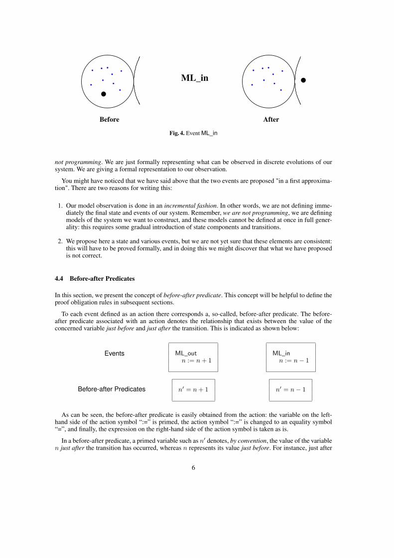
Likewise, Fig. 4 shows the situation just before and just after an occurrence of the second event, ML_in(the name ML_in stands for "getting in the mainland"). As can be seen, the number of cars in the com-pound is decremented as a result of this event:

In a first approximation, we define the events of the initial model in a simple way as follows:

ML_outn := n + 1

ML_inn := n− 1

An event has a name: here ML_out and ML_in. It contains an action: here n := n + 1 and n :=n − 1. These statements can be read as follows: “n becomes equal to n + 1” and “n becomes equal ton − 1”. Such statements are called actions. It is important to notice that in writing these actions we are

5

Before

ML_in

After

Fig. 4. Event ML_in

not programming. We are just formally representing what can be observed in discrete evolutions of oursystem. We are giving a formal representation to our observation.

You might have noticed that we have said above that the two events are proposed "in a first approxima-tion". There are two reasons for writing this:

1. Our model observation is done in an incremental fashion. In other words, we are not defining imme-diately the final state and events of our system. Remember, we are not programming, we are definingmodels of the system we want to construct, and these models cannot be defined at once in full gener-ality: this requires some gradual introduction of state components and transitions.

2. We propose here a state and various events, but we are not yet sure that these elements are consistent:this will have to be proved formally, and in doing this we might discover that what we have proposedis not correct.

4.4 Before-after Predicates

In this section, we present the concept of before-after predicate. This concept will be helpful to define theproof obligation rules in subsequent sections.

To each event defined as an action there corresponds a, so-called, before-after predicate. The before-after predicate associated with an action denotes the relationship that exists between the value of theconcerned variable just before and just after the transition. This is indicated as shown below:

Events

Before-after Predicates

ML_outn := n + 1

n′ = n + 1

ML_inn := n− 1

n′ = n− 1

As can be seen, the before-after predicate is easily obtained from the action: the variable on the left-hand side of the action symbol “:=” is primed, the action symbol “:=” is changed to an equality symbol“=”, and finally, the expression on the right-hand side of the action symbol is taken as is.

In a before-after predicate, a primed variable such as n′ denotes, by convention, the value of the variablen just after the transition has occurred, whereas n represents its value just before. For instance, just after

6

an occurrence of the event ML_out, the value of the variable n is equal to the value it had just before plusone, that is n′ = n + 1.

The before-after predicates we have presented here have got very simple shapes, where the primed valueis equal to some expression depending on the non-primed value. Of course, more complicated shapes canbe encountered but in this example, which is deterministic, we shall not encounter more complicatedcases.

4.5 Proving Invariant Preservation

When writing the actions corresponding to the events ML_in and ML_out, we did not necessarily takeinto account invariants inv0_1 and inv0_2, because we only concentrated in the way the variable n wasmodified. As a consequence, there is no reason a priori for these invariants to be preserved by these events.In fact, it has to be proved in a rigorous fashion. The purpose of this section is thus to define preciselywhat we have to prove in order to ensure that the invariants are indeed invariant!

The statement to be proved is generated in a systematic fashion by means of a rule, called INV, whichis defined once and for all. Such a rule is called a proof obligation rule or a verification condition rule.

Generally speaking, suppose that our constants are collectively called c. And let A(c) denote the axiomsassociated with these constants c. More precisely, A(c) stands for the list: A1(c), A2(c), . . . of axioms as-sociated with the constants. In our example model, A(c) is reduced to a list consisting of the single elementaxm0_1. Likewise, let v denote the variables and let I(c, v) denote the invariants of these variables. As forthe axioms of the constants, I(c, v) stands for the list I1(c, v), I2(c, v), . . . of invariants. In our example,I(c, v) is reduced to a list consisting of the two elements inv0_1 and inv0_2. Finally, let v′ = E(c, v) bethe before-after predicate associated with an event. The invariant preservation statement which we haveto prove for this event and for a specific invariant Ii(c, v) taken from the set of invariants I(c, v) is thenthe following:

A(c), I(c, v) ` Ii(c, E(c, v)) INV

This statement, which is called a sequent (wait till next section for a precise definition of sequents),can be read as follows: “Hypotheses A(c) and hypotheses I(c, v) entail predicate Ii(c, E(c, v))”. This iswhat we have to prove for each event and for each invariant Ii(c, v). It is easy to understand: just beforethe transition, we can assume clearly that each axiom of the set A(c) holds. We can also assume thateach invariant of the set I(c, v) holds too. As a consequence, we can assume A(c) and I(c, v). Now, justafter the transition, where the value of v has been changed to E(c, v), then the invariant statement Ii(c, v)becomes Ii(c, E(c, v)), and it must hold too since it is claimed to be an invariant.

To simplify writing and ease reading, we shall write sequents vertically when there are several hypothe-ses. In the case of our rule INV, this yields the following:

A(c)I(c, v)` INVIi(c, E(c, v))

As this formulation of proof obligation rule INV might seem a bit difficult to remember, let us rewrite itin another way, which is less formal:

7

AxiomsInvariants` INV

Modified Invariant

Proof obligation rule INV states what we have to formally prove in order to be certain that the variousevents maintain the invariants. But we have not yet defined what we mean by "formally prove": this will beexplained in sections 4.8 to 4.11. We shall also explain how we can construct formal proofs in a systematicfashion. Finally, note that such sequents which correspond to applying rule INV is generated easily by atool, which is called a Proof Obligation Generator.

4.6 Sequent

In the previous section, we introduced the concept of sequent in order to express our proof obligation rule.In this section, we give more information about such a construct1. As explained above, a statement of thefollowing form is called a sequent:

H ` G

The symbol ` is named the turnstile. The part situated on the left hand part of the turnstile, here H,denotes a finite set of predicates called the hypotheses (or assumptions). Notice that the set H can beempty. The part situated on the right hand side of the turnstile, here G, denotes a predicate called the goal(or conclusion).

The intuitive meaning of such a statement is that the goal G is provable under the set of assumptionsH. In other words, the turnstile can be read as the verb "entail", or "yield": the assumptions H yield theconclusion G.

In the sequel, we shall always generate such sequents (and try to prove them) in order to analyze ourmodels. We shall also give rules to prove sequents in a formal way.

4.7 Applying the Invariant Preservation Rule

Coming back to our example, we are now in a position to clearly state what we have to prove: this iswhat we are going to do in this section. The proof obligation rule INV we have given in section 4.5 yieldsseveral sequents to prove. We have one application of this proof obligation rule per event and per invariant:in our case, we have two events, namely ML_out and ML_in and we have two invariants, namely inv0_1and inv0_2. This makes four sequents to prove: two sequents for each of the two events.

In order to remember easily what proof obligations we are speaking about, we are going to give com-pound names to them. Such a proof obligation name first mentions the event that is concerned, then theinvariant, and we finally put the label INV in order to remember that it is an invariant preservation proofobligation (as there will be some other kinds of proof obligations2). In our case, the four proof obligationsare thus named as follows:

1 Sequents and the sequent calculus are reviewed in a more formal way in section 1 of Chapter 9.2 All proof obligations are reviewed in section 2 of chapter 5.

8

ML_out / inv0_1 / INV ML_out / inv0_2 / INV

ML_in / inv0_1 / INV ML_in / inv0_2 / INV

Let us now apply proof obligation rule INV to the two events and the two invariants. Here is what wehave to prove concerning event ML_out and invariant inv_01:

Axiom axm0_1Invariant inv0_1Invariant inv0_2`

Modified invariant inv0_1

d ∈ Nn ∈ Nn ≤ d`n + 1 ∈ N

ML_out / inv0_1 / INV

Remember that event ML_out has the before-after predicate n′ = n + 1. This is why predicate n ∈ Ncorresponding to invariant inv0_1 in the assumptions has been replaced by predicate n + 1 ∈ N in thegoal. Here is what we have to prove concerning event ML_out and invariant inv0_2:



d ∈ Nn ∈ Nn ≤ d`n + 1 ≤ d


Here is what we have to prove concerning event ML_in and invariant inv0_1 (remember that the before-after predicate of event ML_in is n′ = n− 1):



d ∈ Nn ∈ Nn ≤ d`n− 1 ∈ N

ML_in / inv0_1 / INV

Here is what we have to prove concerning event ML_in and invariant inv0_2:



d ∈ Nn ∈ Nn ≤ d`n− 1 ≤ d


9

4.8 Proving the Proof Obligations

We know exactly which sequents we have to prove. Our next task is thus now to prove them: this is thepurpose of the present section. The formal proofs of the previous sequents are done by applying sometransformations on sequents, yielding one or several other sequents to prove, until we reach sequents thatare considered being proved without any further justification. The transformation of one sequent into newones corresponds to the idea that proofs of the latter are sufficient to prove the former. For example, ourfirst sequent, namely:

d ∈ Nn ∈ Nn ≤ d`n + 1 ∈ N

(1)

can be simplified by removing some irrelevant hypotheses (clearly hypotheses d ∈ N and n ≤ d areuseless for proving our goal n + 1 ∈ N), yielding the following simpler sequent:

n ∈ N ` n + 1 ∈ N (2)

What we have admitted here as a step in the proof is the fact that a proof of sequent (2) is sufficient toprove sequent (1). In other words, if we succeed now proving sequent (2), then we have also a proof ofsequent (1). The proof of the sequent (2) is reduced to nothing. In other words, it is accepted as beingproved without further justification. It says that, under the assumption that n is a natural number, thenn + 1 is also a natural number.

4.9 Rules of Inference

In the previous section, we applied informally some rules either to transform a sequent into another one orto accept a sequent without further justification. Such rules can be rigorously formalized, they are calledrules of inference: this is what we do in the present section. The first rule of inference we have used canbe stated as follows:

H1 ` G

H1, H2 ` GMON

Here is the structure of such a rule. On top of the horizontal line, we have a set of sequents (here justone). These sequents are called the antecedents of the rule. Below the horizontal line, we always have asingle sequent called the consequent of the rule. On the right of the rule we have a name, here MON: thisis the name of the inference rule. In this case, this name stands for monotonicity of hypotheses.

The rule is to be read as follows: in order to prove the consequent, it is sufficient to have proofs of eachsequent in the antecedents. In the present case, it says that in order to have a proof of goal G under the

10

two sets of assumptions H1 and H2, it is sufficient to have a proof of G under H1 only. We have indeedobtained the effect we wanted: the removing of possibly irrelevant hypotheses H2.

Note that in applying this rule we do not require that the subset of assumptions H2 is entirely situatedafter the subset H1 as is strictly indicated in the rule. In fact, the subset H2 is to be understood as anysubset of the hypotheses. For example, in applying this rule to our proof obligation (1) in the previoussection we removed the assumption d ∈ N situated before assumption n ∈ N, and assumption n ≤ dwhich was situated after it.

The second rule of inference can be stated as follows:

H, n ∈ N ` n + 1 ∈ NP2

Here we have a rule of inference with no antecedent. For this reason, it is called an axiom. This is thesecond Peano Axiom for natural numbers, hence the name P2. It says that in order to have a proof of theconsequent it is not necessary to prove anything. Under the hypothesis that n is a natural number then n+1is also a natural number. Notice that the presence of the additional hypotheses H is optional here. This isso because it is always possible to remove the additional hypotheses using rule MON. Thus the rule couldhave been stated more simply as follows (this is the convention we shall follow in the sequel):

n ∈ N ` n + 1 ∈ NP2

A similar but more constraining rule will be used in the sequel. It concerns decrementing a natural number:

0 < n ` n− 1 ∈ NP2′

This rule says that n −1 is a natural number under the assumption that n is positive. We shall also use twoother rules of inference called INC and DEC

n < m ` n + 1 ≤ mINC

Rule of inference INC says that n +1 is smaller than or equal to m under the assumption that n is strictlysmaller than m.

n ≤ m ` n− 1 < mDEC

11

Rule of inference DEC says that n −1 is smaller than m under the assumption that n is already smallerthan or equal to m. We shall clearly need more rules of inference dealing with elementary logic and alsowith natural numbers. But for the moment, we only need those we have just presented in this section.

Notice that it is well known that inference rules P2’, INC and DEC are derived inference rules: it simplymeans that such inference rules can be deduced from more basic inference rules such as P2 above andothers. But in this presentation, we are not so much interested in this: we want just to construct a libraryof useful inference rules

4.10 Meta-variables

You might have noticed that the various identifiers, namely H1,H2, G, n, m we have used in the rules ofinferences proposed in the previous section, were emphasized: we have not used the standard mathemati-cal font for them, namely H1,H2, G, n, m. This is because such variables are not part of the mathematicallanguage we are using. They are called meta-variables.

More precisely, each proposed rule of inference stands for a schema of rules corresponding to all thepossible matches we could ever perform. For example rule P2:

n ∈ N ` n + 1 ∈ NP2

describes the second Peano axiom in very general terms: it can be applied to the sequent

a + b ∈ N ` a + b + 1 ∈ N

by matching meta-variable n to the mathematical language expression a + b.

4.11 Proofs

Equipped with a number of rules of inference, we are now ready to perform some elementary formalproofs: this is the purpose of this section. A proof is just a sequence of sequents connected by the name ofthe rule of inference which allows one to go from one sequent to the next in the sequence. The sequenceof sequents ends with the name of a rule of inference with no antecedent. We shall see in section 4.24 thatproofs have a more general shape but that one is sufficient for the moment.

For example, the proof of our first proof obligation ML_out / inv0_1 / INV is the following. It corre-sponds exactly to what has been said informally in section 4.8, namely removing some useless hypothesesand then accepting the second sequent without any further proof:

d ∈ Nn ∈ Nn ≤ d`n + 1 ∈ N

MONn ∈ N`n + 1 ∈ N

P2

12

The next proof, corresponding to proof obligation ML_out / inv0_2 / INV, fails because we cannotapply rule INC on the final sequent as we do not have an assumption telling us that n < d holds asrequired by rule INC: we only have the weaker assumption n ≤ d. For this reason, we have put a "?" atthe end of the sequence of sequents:

d ∈ Nn ∈ Nn ≤ d`n + 1 ≤ d

MONn ≤ d`n + 1 ≤ d

?

Likewise, the proof of ML_in / inv0_1 / INV fails. Here we cannot apply inference rule P2’ on the lastsequent because we do not have the required assumption 0 < n, only the weaker one n ∈ N:

d ∈ Nn ∈ Nn ≤ d`n− 1 ∈ N

MONn ∈ N`n− 1 ∈ N

?

The last proof, that of ML_in / inv0_2 / INV, succeeds:

d ∈ Nn ∈ Nn ≤ d`n− 1 ≤ d

MONn ≤ d`n− 1 < d ∨ n− 1 = d

OR_R1n ≤ d`n− 1 < d

DEC

Notice that in the second step we felt free to replace n− 1 ≤ d, that is n− 1 is smaller than or equal tod, by the equivalent formal statement n− 1 < d ∨ n− 1 = d, where ∨ is the disjunctive operator "or".Then, we apply inference rule OR_R1 (see next section) in order to obtain the goal n − 1 < d which iseasily proved using rule DEC.

4.12 More Rules of Inference

At the end of previous section, we apply our first logical rule of inference named OR_R13. In the sequel,there will be more logical rules of inference, but this one is the first one we need. We present it togetherwith the companion rule OR_R2:

H ` P

H ` P ∨QOR_R1

H ` Q

H ` P ∨QOR_R2

3 All rules of inference are reviewed in Chapter 9.

13

Both rules state obvious facts about proving a disjunctive goal P ∨ Q involving two predicates P and Q.For proving their disjunction, it is sufficient to prove one of them: P in the case of rule OR_R1 and Q inthe case of rule OR_R2.

Notice that in the _R1 or _R2 suffixes of these rule names, the R stands for "right": it means that thisrule transforms a goal, that is a statement situated on the right hand side of the turnstile. Other logicalinference rules presented below will be named using the suffix L when the transformed predicate is anhypothesis, that is a predicate situated on the left hand side of the turnstile.

4.13 Improving the two Events: Introducing Guards

Coming back to our example, we have now to do some modifications in our model due to the fact thatsome proofs have failed. We figure out that proving has the same effect as debugging. In other words, afailed proof reveals a bug.

In order to correct the deficiencies we have discovered while carrying out the proof, we have to addguards to our events. Together, these guards denote the necessary conditions for an event to be enabled.More precisely, when an event is enabled, it means that the transition corresponding to the event can takeplace. On the contrary, when an event is not enabled (that is when at least one of its guards does not hold)it means that the corresponding transition cannot occur.

For event ML_out to be enabled, we shall require that n be strictly smaller than d, that is n < d. Andfor event ML_in to be enabled, we shall require that n be strictly positive, that is 0 < n. Notice that suchguarding conditions are exactly the conditions that were missing in the sequents we had to prove in theprevious section: we have been guided by the failure of the proofs. Adding guards to events is done asfollows:

ML_outwhen

n < dthen

n := n + 1end

ML_inwhen

0 < nthen

n := n− 1end

As can be seen, we have a simple piece of syntax here: the guard is situated between the keywords whenand then, whereas the action is situated between the keywords then and end. Note that we may haveseveral guards in an event, although it is not the case here.

4.14 Improving the Invariant Preservation Rule

When dealing with a guarded event with the set of guards denoted by G(c, v) and before-after predicateof the form v′ = E(c, v) (where c denotes the constants and v the variables as introduced in section4.5), our previous proof obligation rule INV has to be modified by adding the set of guards G(c, v) to thehypotheses of the sequent. This yields the following more general proof obligation for events that haveguards:

A(c)I(c, v)G(c, v) INVÌi(c, E(c, v))

AxiomsInvariantsGuards of the event INV`

Modified Invariant

14

4.15 Reproving Invariant Preservation

The statements to prove by applying the amended proof obligation rule INV are modified accordingly andare now easily provable. Here is the sequent to prove for ensuring that event ML_out preserves invariantinv0_2:

Axiom axm0_1Invariant inv0_1Invariant inv0_2Guard of ML_out`


d ∈ Nn ∈ Nn ≤ dn < d`n + 1 ≤ d


Here is what we have to prove concerning event ML_in and invariant inv0_1

Axiom axm0_1Invariant inv0_1Invariant inv0_2Guard of ML_in`


d ∈ Nn ∈ Nn ≤ d0 < n`n− 1 ∈ N


The two missing proofs can now be performed easily:

d ∈ Nn ∈ Nn ≤ dn < d`n + 1 ≤ d

MONn < d`n + 1 ≤ d

INC

d ∈ Nn ∈ Nn ≤ d0 < n`n− 1 ∈ N

MON0 < n`n− 1 ∈ N

P2’

Notice that the proofs we have already done for proof obligations ML_out / inv0_1 / INV and ML_in /inv0_2 / INV in section 4.11 need not to be redone. This is because we are just adding a new hypothesisto these proof obligations: remember inference rule MON (section 4.9) which says that for proving a goalunder certain hypotheses H, it is sufficient to perform the proof of the same goal under less hypotheses.So, conversely adding an hypothesis to a proof which is already done does not invalidate that proof.

15

4.16 Initialization

In the previous sections, we defined the two events ML_in and ML_out and the invariants of the model,namely inv0_1 and inv0_2. We also proved that these invariants were preserved by the transition definedby the events. But we have not defined what happens at the beginning. For this, it is necessary to define aspecial initial event that is systematically named init. In our case, this event is the following:

initn := 0

As can be seen, the initializing event corresponds to the observation that initially there are no cars in thecompound. Notice that this event has no guard: this must always be the case with the initializing eventinit. In other words, initialization must always be possible!

Also note that the expression situated on the right hand sign of := in the action of the event init cannotrefer to any variable of the model. This is because we are initializing. In our case, the variable n cannotbe assigned an expression depending on n. The corresponding before-after predicate of init is thus alwaysrather an "after predicate" only. In our case, it is the following (as can be seen, this predicate does notmention n, only n′):

n′ = 0

4.17 Invariant Establishment Rule for the Initializing Event init

Event init cannot preserve the invariants because before init the system state “does not exist”. Event initmust just establish the invariant for the first time. In this way, other events, which by definition are onlyobservable after initialization has taken place, can be enabled in a situation where the invariants hold.

We have thus to define a proof obligation rule for this invariant establishment. It is almost identical tothe proof obligation rule INV we have already presented in section 4.5. The difference is that in the proofobligation rule presented now the invariants are not mentioned in the hypotheses of the sequent. Moreprecisely, given a system with constants c, with a set of axioms A(c), with variables v and an invariantIi(c, v), and an initializing event with after predicate v′ = K(c), then the proof obligation rule INV forinvariant establishment is the following:

A(c)` INVIi(c,K(c))

Axioms` INV

Modified Invariant

4.18 Applying the Invariant Establishment Rule

The application of the previous rule to our initializing event init yields the following to prove:

16

Axiom axm0_1`

Modified Invariant inv0_1d ∈ N ` 0 ∈ N inv0_1 / INV

Axiom axm0_1`

Modified Invariant inv0_2d ∈ N ` 0 ≤ d inv0_2 / INV

4.19 Proving the Initialization Proof Obligations: More Inference Rules

The proof obligations of the previous section cannot be formally proved without other inference rules.The first one is named P1: it is the first Peano axiom, which says that 0 is a natural number. Notice thatthe sequent that defines the consequent of this inference rule has no assumption:

` 0 ∈ NP1

The second rule of inference we need is a consequence of the third Peano axiom which says that 0 is notthe successor of any natural number. We can prove that this can be re-phrased as follows: 0 is the smallestnatural number. In other words, under the assumption that n is a natural number then 0 is smaller than orequal to n. For convenience, we shall name it P3:

n ∈ N ` 0 ≤ nP3

We leave it as an exercise to the reader to now prove the two previous initialization proof obligations.

4.20 Deadlock Freedom

Since our two main events ML_in and ML_out are now guarded, it means that our model might deadlockwhen both guards are false: none of the events would be enabled, the system would be blocked. Sometimesthis is what we want, but certainly not here, where this is to be avoided. As a matter of fact, we discoverthat this non-blocking property was missing in our requirement document of section 2. So we edit thisdocument by adding this new requirement:

Once started, the system should work for ever FUN-4

17

4.21 Deadlock Freedom Rule

Given a model with constants c, set of axioms A(c), variables v and set of invariants I(c, v), we have thusto prove a proof obligation rule called DLF (for deadlock freedom) stating that one of the guards G1(c, v),. . . , Gm(c, v) of the various events is always true. In other words, in our case, cars can always either enterthe compound or leave it. This is to be proved under the set of axioms A(c) of the constants c and underthe set of invariants I(c, v). The proof obligation rule can be stated as follows in general terms:

A(c)I(c, v)` DLFG1(c, v) ∨ . . . ∨ Gm(c, v)

AxiomsInvariants` DLF

Disjunction of the guards

Note that the application of this rule is not mandatory: not all systems need to be deadlock free.

4.22 Applying the Deadlock Freedom Proof Obligation Rule

Here is what we have to prove according to rule DLF:


Disjunction of the guards

d ∈ Nn ∈ Nn ≤ d`n < d ∨ 0 < n

DLF

4.23 More Inference Rules

The previous deadlock freedom proof obligation cannot be proved without more rules of inference. Thefirst one is a logical rule, which corresponds to the classical technique of a proof by cases. It is namedOR_L as it has to do with the "or" symbol ∨ situated in the "Left" hand assumption part of a sequent.Notice that the antecedent of this rule has two sequents. More precisely, in order to prove a goal under adisjunctive assumption P ∨ Q, it is sufficient to prove independently the same goal under assumption Pand also under assumption Q:

H, P ` R H, Q ` R

H, P ∨Q ` ROR_L

For the sake of completeness, we provide again the two logical inference rule we have already presentedin section 4.12:

H ` P

H ` P ∨QOR_R1

H ` Q

H ` P ∨QOR_R2

18

Our last logical rules have to do with the essence of a sequent.The first rule, HYP says that when thegoal of a sequent is present as an assumption of that sequent then the sequent is proved. The second rule,FALSE_L, says that a sequent with a false assumption is proved. We denote false with the symbol ⊥.

P ` PHYP

⊥ ` PFALSE_L

Our next two rules of inference are dealing with equality. They explain how one can exploit an assumptionwhich is an equality.

H(F), E = F ` P(F)

H(E), E = F ` P(E)EQ_LR

H(E), E = F ` P(E)

H(F), E = F ` P(F)EQ_RL

In rule EQ_LR, we have a sequent with a goal P(E), which is a predicate depending on the expression E.We also have a set of hypotheses H(E) depending of E. Finally, we have the equality hypothesis E = F.The rule says that we can then replace this sequent by another one where all occurrences of E in P(E) andin H(E) have been replaced by F. The label LR is to remember that we apply the equality from "Left" to"Right". Rule EQ_RL exploits the same equality by applying it now from right to left, that is replacing Fby E in P(F) and H(F) yielding P(E) and H(E). Note that we have not formally explained exactly whatwe mean when we say that a predicate "depends" on an expression E. This will be made more preciselater.

Our last rule, dealing with equality, says that any expression E is equal to itself. This rule in not usedimmediately in the next proof but it is quite natural to introduce it now:

` E = EEQL

4.24 Proving the Deadlock Freedom Proof Obligation

Coming back to our example, we are going to give a tentative proof of our deadlock freedom proofobligation DLF, which we repeat below:

d ∈ Nn ∈ Nn ≤ d`n < d ∨ 0 < n

DLF

Here, we are going to apply inference rule OR_L because the assumption n ≤ d is in fact equivalent tothe disjunctive predicate n < d ∨ n = d. As can be seen, the usage of inference rule OR_L induces a

19

tree shape to the proof. This is because we have two antecedents in this rule. This tree shape is the normalshape of a proof:

d ∈ Nn ∈ Nn < d ∨ n = d`n < d ∨ 0 < n

MONn < d ∨ n = d`n < d ∨ 0 < n

OR_L . . .

· · ·

n < d`n < d ∨ 0 < n

OR_R1 n < d ` n < d HYP

n = d`n < d ∨ 0 < n

EQ_LR ` d < d ∨ 0 < d OR_R2 ` 0 < d ?

We now discover that the last sequent cannot be proved. We have thus to add the following axiom, namedaxm0_2, which was obviously forgotten:

axm0_2: 0 < d

We notice that this additional axiom allows us to have a more precise requirement FUN-2:

The number of cars on bridge and island is limited but positive FUN-2

Adding this axiom to avoid deadlock is very intuitive because when d is equal to 0 then the system isdeadlocked right from the beginning since no car can ever enter the compound. Again, note that addingthis new axiom for the constant d does not invalidate the proofs we have already made so far: this is aconsequence of the monotonicity rule MON introduced in section 4.9.

4.25 Conclusion and Summary of the Initial Model

As we have seen, the proofs (or rather the failed proof attempts) allowed us to discover that our eventswere too naive (we had to add guards in section 4.13) and also that one axiom was missing for constantd (previous section). This is quite frequently the case: proofs help discovering inconsistencies in a model.In fact, this is the heart of the modeling method! Here is the final version of the state for our initial model:

constant: daxm0_1: d ∈ N

axm0_2: d > 0variable: n

inv0_1: n ∈ N

inv0_2: n ≤ d

20

And here are the final version of the events of our initial model:

initn := 0

ML_outwhen

n < dthen

n := n + 1end

ML_inwhen

0 < nthen

n := n− 1end

5 First Refinement: Introducing the One Way Bridge

5.1 Introduction

We are now going to proceed with a refinement of our initial model. A refinement is a more precise modelthan the initial one. It is more precise but it should not contradict the initial model. Therefore we shallcertainly have to prove that the refinement is consistent with the initial model. This will be made clear inthis section.

In this first refinement, we introduce the bridge. This means that we are able to observe more accuratelyour system. Together with this more accurate observation, we can also see more events, namely carsentering and leaving the island. These events are called IL_in and IL_out. Note that events ML_out andML_in, which were present in the initial model, still exist in this refinement: they now correspond to carsleaving the mainland and entering the bridge or leaving the bridge and entering the mainland. All this isillustrated in Fig. 5.

I s l a n d

ML_outIL_in

ML_inIL_out

one way

Bridge

Fig. 5. Island and Bridge

5.2 Refining the State

The state, which was defined by the constant d and variable n in the initial model, now becomes moreaccurate. The constant d remains, but the variable n is now replaced by three variables. This is becausenow we can see cars on the bridge and in the island, something which we could not distinguish in theprevious abstraction. Moreover, we can see where cars on the bridge are going: either towards the islandor towards the mainland.

21

For these reasons, the state is now represented by means of three variables a, b, and c. Variable adenotes the number of cars on the bridge and going to the island, variable b denotes the number of carsin the island, and variable c denotes the number of cars on the bridge and going to the mainland. This isillustrated in Fig. 6.

ba

c

Fig. 6. The Concrete State

The state of the initial model is called the abstract state and the state of the refined model is called theconcrete state. Likewise, variable n of the abstract state is called an abstract variable whereas variablesa, b, and c of the concrete state are called concrete variables.

The concrete state is represented by a number of invariants, which we call the concrete invariants. First,variables a, b, and c are all natural numbers. This is stated in invariants inv1_1, inv1_2, and inv1_3 below.

variables: a, b, c

inv1_1: a ∈ N

inv1_2: b ∈ N

inv1_3: c ∈ N

inv1_4: a + b + c = n

inv1_5: a = 0 ∨ c = 0

Then we express that the sum of these variables is equal to the previous abstract variable n which hasdisappeared. This is expressed in invariant inv1_4. This invariant relates the concrete state represented bythe three variables a, b, and c, to the abstract state represented by the variable n. And finally, we state thatthe bridge is one-way: this is our basic requirement FUN-3. This is expressed by saying that a or c areequal to zero. Clearly they cannot be both positive since the bridge is one-way, but they can be both equalto zero if the bridge is empty. This one-way property is expressed in invariant inv1_5.

Notice that among the concrete invariants some are dealing with the concrete variables only, these areinv1_1, inv1_2, inv1_3, and inv1_5, and one is dealing with concrete and abstract variables, this is inv1_4.

5.3 Refining the Abstract Events

The two abstract events ML_out and ML_in now have to be refined as they are not dealing with theabstract variable n anymore but with the concrete variables a, b, and c. Here is the proposed concreteversions (sometimes also called refined versions) of events ML_in and ML_out:

22

ML_inwhen

0 < cthen

c := c− 1end

ML_outwhen

a + b < dc = 0

thena := a + 1

end

Notice that event ML_out has two guards, namely a + b < d and c = 0. Also notice that although ourrefined model has now three variables a, b, and c, only one of them is mentioned in each event: c in eventML_in and a in event ML_out. In fact, the other two are, in each case, implicitly mentioned as being leftunchanged.

It is easy to understand what these events are doing. In event ML_in, the action decrements variable cas there will be one car less on the bridge, and this can be done if there are some cars on the bridge goingto the mainland, that is when 0 < c holds (notice that we are sure that there are no cars on the bridgegoing to the island as a must be equal to 0 since c is positive).

In event ML_out, the action increments variable a as there will be one more car on the bridge. But thisis possible only if c is equal to 0, because of the one-way constraint of the bridge. Moreover, this will alsobe possible only if the new car entering the bridge does not break the constraint that there are a maximumnumber of d cars in the compound, that is when a + b + c < d holds, which reduces to a + b < d since cis equal to 0.

5.4 Revisiting the Before-after Predicates

The observation concerning the actions of the concrete events in the previous section makes us be moreprecise now concerning the construction of the before-after predicate. The before-after predicate of theaction corresponding to an event situated in a model containing several variables must mention explicitlythat the missing variables in the action are not modified: this is done by stating that their primed after-values are equal to their non-primed before-values. In the case of our example, the following before-afterpredicates are associated with the corresponding event actions as follows:

Events

Before-AfterPredicates

ML_inwhen

0 < cthen

c := c− 1end

a′ = a ∧ b′ = b ∧ c′ = c− 1

ML_outwhen

a + b < dc = 0

thena := a + 1

end

a′ = a + 1 ∧ b′ = b ∧ c′ = c

As can be seen, the before after-predicate of the action c := c− 1 contains c′ = c− 1 as expected but alsoa′ = a and b′ = b. We have similar equalities corresponding to the action a := a + 1.

23

5.5 Informal Proofs of Refinement

In the next section, we shall clearly define what is required for the concrete version of an event to refineits abstraction. In this section, we are just presenting some informal arguments. For this, we are going tocompare the abstract and concrete versions of our two events respectively. Here are the two versions ofthe event ML_out:

(abstract_)ML_outwhen

n < dthen

n := n + 1end

(concrete_)ML_outwhen

a + b < dc = 0

thena := a + 1

end

As can be seen, the concrete version of this event has guards which are completely different from thatof the abstraction. We can already “feel” that the concrete version is not contradictory with the abstractone. When the concrete version is enabled, that is when its guards hold, then certainly the abstract one isenabled too. This is so because the two concrete guards a+b < d and c = 0 together imply a+b+c < d,that is n < d, which is the abstract guard, according to invariant inv1_4 which states that a + b + c isequal to n. Moreover, when a is incremented and the other variables left unchanged as stated in the actiona := a+1 in the concrete version, this clearly corresponds to the fact that n is incremented in the abstractone, according again to the invariant inv1_4. Likewise, here are the two versions of the event ML_in:

(abstract_)ML_inwhen

0 < nthen

n := n− 1end

(concrete_)ML_inwhen

0 < cthen

c := c− 1end

A similar informal "proof" can be conducted on these two versions of event ML_in showing that theconcrete one does not contradict the abstract one.

5.6 Proving the Correct Refinements of Abstract Events

In this section, we are going to give systematic rules defining exactly what we have to prove in order toensure that a concrete event indeed refines its abstraction. In fact, we have to prove two different things.First a statement concerning the guards, and second a statement concerning the actions.

Guard Strengthening We first have to prove that the concrete guard is stronger than the abstract one.The term “stronger” means that the concrete guard implies the abstract guard. In other words, it is notpossible to have the concrete version enabled whereas the abstract one would not. Otherwise, it would bepossible to have a concrete transition with no counterpart in the abstraction. This has to be proved underthe abstract axioms of the constants, the abstract invariants and the concrete invariants. We shall see insection 5.16 that we cannot strengthen the refined guards too much because it might result in unwanteddeadlocks.

24

In more general terms, let c denote the constants, A(c) the set of constant axioms, v the abstract vari-ables, I(c, v) the set of abstract invariants, w the concrete variables, J(c, v, w) the set of concrete in-variants. Let an abstract event have the set of guards G(c, v). In other words, G(c, v) stands for the listG1(c, v), G2(c, v), . . .. Let the corresponding concrete event have the set of guard H(c, w). We have thento prove the following for each concrete guard Gi(c, v):

A(c)I(c, v)J(c, v, w) GRDH(c, w)`Gi(c, v)

AxiomsAbstract invariantsConcrete invariants GRDConcrete guards`

Abstract guard

Notice again that the set of concrete invariants denoted by J(c, v, w) contain some elementary invariantsdealing with concrete variables w only, while others are dealing with both abstract and concrete variablesv and w. This is the reason why we collectively denote this set of concrete invariants by J(c, v, w).

Also note that it is possible to introduce new constants in a refinement. But we have not stated this inthe concrete invariants J(c, v, w) in order to keep the formulae small.

Correct Refinement We have to prove that the concrete event transforms the concrete variables w intow′, in a way which does not contradict the abstract event. While this transition happens, the abstract eventchanges the concrete variables v, which are related to w by the concrete invariant J(c, v, w), into v′, whichmust be related to w′ by the modified concrete invariant J(c, v′, w′). This is illustrated in the followingdiagram:

v

w

Abstract Event

Concrete Event

J(c,v,w)

I(v) I(v’)

J(c,v’,w’)

v’=E(c,v)

w’=F(c,w)H(c,w)

G(c,v)

With our usual conventions, this leads to the following proof obligation rule named INV, where Jj(c, v, w)denotes a single invariant of the set of concrete invariants J(c, v, w).

A(c)I(c, v)J(c, v, w)H(c, w) INV`Jj(c, E(c, v), F (c, w))

AxiomsAbstract invariantConcrete invariantConcrete guard INV`

Modified concrete invariant

25

5.7 Applying the Refinement Rules

Coming back to our example, we apply rule GRD to both refined events ML_out and ML_in. This leadsto some sequents, which look complicated but are easy to prove.

Applying guard strengthening to Event ML_out. Here is what we have to prove for event ML_out:

axm0_1axm0_2inv0_1inv0_2inv1_1inv1_2inv1_3inv1_4inv1_5Concrete guards of ML_out

Àbstract guards of ML_out

d ∈ N0 < dn ∈ Nn ≤ da ∈ Nb ∈ Nc ∈ Na + b + c = na = 0 ∨ c = 0a + b < dc = 0`n < d

ML_out / GRD

This huge impressive sequent can be dramatically simplified. First, we can remove useless hypothesesby applying MON. Then we can apply the equality present in hypothesis, that is c = 0, thus transforminghypothesis a+b+c = n first into a+b+0 = n and then into a+b = n. Then, we can apply this equality,thus replacing hypothesis a + b < d by the simpler one n < d. And now we discover that this is exactlythe goal we wanted to prove: we can apply HYP. More formally, this leads to the following successivetransformations of our original sequent (obtained after applying rule MON):

a + b + c = na + b < dc = 0`n < d

EQ_LR

a + b + 0 = na + b < d`n < d

ARI

a + b = na + b < d`n < d

EQ_LRn < d`n < d

HYP

As can be seen, we have introduced a generic rule of inference named ARI. This is to say in a less formalway that the justification is based on simple arithmetic properties. We could have defined correspondingspecific rules of inference but there is no point in doing this here for the moment. In order to make clearwhich arithmetic properties we are thinking of, the relevant assumptions or goal are underlined in thesequent situated to the left of this ARI justification.

Applying guard strengthening to Event ML_in. After applying MON, we obtain the following sequent:

b ∈ Na + b + c = na = 0 ∨ c = 00 < c`0 < n

26

The disjunctive assumption suggests doing a proof by cases. Then we may apply the equalities, thussimplifying the sequents to prove. The proof is finished by applying a number of simple arithmetic trans-formations. Here is the proof of this sequent:

b ∈ Na + b + c = na = 0 ∨ c = 00 < c`0 < n

OR_L

b ∈ Na + b + c = na = 00 < c`0 < n

EQ_LR

b ∈ N0 + b + c = n0 < c`0 < n

ARI . . .

b ∈ Na + b + c = nc = 00 < c`0 < n

EQ_LR

b ∈ Na + b + 0 = n0 < 0`0 < n

MON . . .

. . .

b ∈ Nb + c = n0 < c`0 < n

ARI

c ≤ n0 < c`0 < n

ARI0 < n`0 < n

HYP

. . .0 < 0`0 < n

ARI⊥`0 < n

FALSE_L

Applying proof obligation rule INV leads to ten predicates to prove since we have two events and fiveconcrete invariants. We shall only present some of them, the other being left as exercises to the reader.

Invariant inv1_4 preservation with Event ML_out. After applying MON, here is the proof we obtain:

a + b + c = nà + 1 + b + c = n + 1

ARIa + b + c = nà + b + c + 1 = n + 1

EQ_LR ` n + 1 = n + 1 EQL

Invariant inv1_5 preservation with Event ML_in. After applying MON, here is the proof we obtain:

27

a = 0 ∨ c = 00 < cà = 0 ∨ c− 1 = 0

OR_L

a = 00 < cà = 0 ∨ c− 1 = 0

OR_R1

a = 00 < cà = 0

MONa = 0à = 0

HYP

c = 00 < cà = 0 ∨ c− 1 = 0

EQ_LR · · ·

· · · 0 < 0 ` a = 0 ∨ −1 = 0 ARI ⊥ ` a = 0 ∨ −1 = 0 FALSE_L

5.8 Refining the Initialization Event Init

We also have to define the refinement of the special event init. This event can be stated obviously asfollows:

inita := 0b := 0c := 0

Here we see for the first time a multiple action. The corresponding before-after predicate is what weexpect:

a′ = 0 ∧ b′ = 0 ∧ c′ = 0

5.9 Correct Proof Obligation Refinement Rule for the Initialization Event init

The proof obligation rule we have to apply in the case of the init event is a special case of the proofobligation rule INV. It is also called INV. If the abstract initialization has an after predicate of the formv′ = K(c) and the concrete initialization has an after predicate of the form w′ = L(c), then the proofobligation rule is the following:

A(c)` INVJj(c,K(c), L(c))

Axioms` INV

Modified concrete invariant

Notice that we have no proof obligation rule for guard strengthening since, by definition, the initializationevent is not guarded.

28

5.10 Applying the Initialization Proof Obligation Refinement Rule

The application of the proof obligation rule introduced in the previous section is straightforward in ourexample. Out of the five predicates, we give only the most important ones. Here is what we have to proveconcerning invariant inv1_4:

axm0_1axm0_2`

Modified concrete invariant inv1_4

d ∈ Nd > 0`0 + 0 + 0 = 0

inv1_4 / INV

Here is what we have to prove concerning invariant inv1_5:

axm0_1axm0_1`

Modified concrete invariant inv1_5

d ∈ Nd > 0`0 = 0 ∨ 0 = 0

inv1_5 / INV

The proofs of these sequents are left to the reader.

5.11 Introducing New Events

We now have to introduce some new events corresponding to cars entering and leaving the island. Nextare the proposed new events:

IL_inwhen

0 < athen

a := a− 1b := b + 1

end

IL_outwhen

0 < ba = 0

thenb := b− 1c := c + 1

end

We have here again some multiple actions. These actions are incomplete however since in the first onevariable c is missing, whereas variable a is missing in the second one. Such multiple actions are associatedwith the following before-after predicates:

a′ = a− 1 ∧ b′ = b + 1 ∧ c′ = c a′ = a ∧ b′ = b− 1 ∧ c′ = c + 1

29

It is also easy to understand what these events are doing. Event IL_in corresponds to a car leavingthe bridge and entering the island. The action thus decrements the number a of cars on the bridge andsimultaneously increments the number b of cars on the island. But this can only be done when there arecars on the bridge, that is when the condition 0 < a holds.

Event IL_out corresponds to a car leaving the island and entering the bridge. The action clearly de-creases b and simultaneously increases c. But this can be done only if there are cars on the island, that isif the condition 0 < b holds. A second condition for event IL_out to be enabled is that there are no carson the bridge going to the island (remember, the bridge is one-way), that is if the condition a = 0 holds.

5.12 The Empty Action skip

As we shall explain in the next section, the new events have to be proved to refine a “dummy event” thatis non-guarded and does nothing in the abstraction. Such a void action is denoted by means of the emptyaction skip.

It is very important to note that the before-after predicate of skip depends on the state of the model inwhich it is located. In the present case, we shall speak first of such an empty action in the initial modelwhich has the single variable n. Its before-after predicate is thus the following:

n′ = n

But a skip action residing in the concrete state, where we have the three variables a, b, and c, would beassociated with the following different before-after predicate:

a′ = a ∧ b′ = b ∧ c′ = c

5.13 Proving that the New Events are Correct

The new events that we have introduced in section 5.11 were not visible in the abstraction. Although notvisible, it does not mean that they did not exist and occur. When you are looking through a microscopeyou can see things that were not visible without the microscope. By analogy, refinement is the same thingas looking a system through a microscope. The transitions corresponding to the new events IL_in andIL_out were not visible in the abstraction but, again, they existed. Formalizing this idea consists in sayingthat the new events refine a non-guarded event with the empty action skip. As a consequence, we can useproof obligation rule INV to prove that our new events are correct. Here is what we have to prove for eventIL_in and concrete invariant inv1_4:

30

axm0_1axm0_2inv0_1inv0_2inv1_1inv1_2inv1_3inv1_4inv1_5Concrete guards of IL_in`

Modified Invariant inv1_4

d ∈ N0 < dn ∈ Nn ≤ da ∈ Nb ∈ Nc ∈ Na + b + c = na = 0 ∨ c = 00 < aà− 1 + b + 1 + c = n

IL_IN / inv1_4 / INV

Notice that n is not modified as the event refines a non-guarded event with a skip action in the abstraction.After applying MON, we obtain the following proof:

a + b + c = nà− 1 + b + 1 + c = n

ARIa + b + c = nà + b + c = n

HYP

Here is what we have to prove for event IL_in and concrete invariant inv1_5:

· · ·inv1_1inv1_2inv1_3inv1_4inv1_5Concrete guards of IL_in`

Modified Invariant inv1_5

· · ·a ∈ Nb ∈ Nc ∈ Na + b + c = na = 0 ∨ c = 00 < aà− 1 = 0 ∨ c = 0

IL_IN / inv1_5 / INV

After applying MON, we obtain the following proof:

a = 0 ∨ c = 00 < aà− 1 = 0 ∨c = 0

OR_L

a = 00 < aà− 1 = 0 ∨c = 0

EQ_LR

0 < 0`−1 = 0 ∨c = 0

ARI

⊥`−1 = 0 ∨c = 0

FALSE_L

c = 00 < aà− 1 = 0 ∨ c = 0

OR_R2

c = 00 < a`c = 0

MONc = 0`c = 0

HYP

We leave it as an exercise to the reader to state and prove the remaining sequents corresponding to theother predicates and the other new event IL_out.

31

5.14 Proving the Convergence of the New Events

In the case where we introduce some new events, we have to prove something else, namely that they donot diverge. In other words, the new events must not be indefinitely enabled. Should it be the case, then theconcrete versions of the existing events, here ML_out and ML_in, could be postponed indefinitely, whichis certainly something we want to avoid since such events could possibly occur in the abstraction. Forproving this, we have to exhibit a natural number expression called a variant and prove that it is decreasedby all new events. This leads to two proof obligation rules: one states that the proposed variant is a naturalnumber and the other states that the variant is decreased by the new events.

In the first proof obligation rule, called NAT, we prove that the exhibited variant V (c, w) is a naturalnumber. This is to be done assuming the axioms A(c) of the constants c, the abstract invariants I(c, v),the concrete invariants J(c, v, w) and the guards of each new event H(c, w). The guard H(c, w) is put inthe antecedent as we are not interested in proving that the exhibited variant is a natural number when theguard of a new event does not hold (it could be negative in this case).

A(c)I(c, v)J(c, v, w)H(c, w) NAT`V (c, w) ∈ N

AxiomsAbstract invariantsConcrete invariantsConcrete guards of a new event NAT`

Variant ∈ N

The second proof obligation rule states that the variant V (c, w) is decreased. This has to be proved foreach new event with guards H(c, w) and before-after predicate w′ = F (c, w):

A(c)I(c, v)J(c, v, w)H(c, w) VAR`V (c, F (c, w)) < V (c, w)

AxiomsAbstract invariantsConcrete invariantsConcrete guards of a new event VAR`

Modified Variant < Variant

Note that the variant is unique. In other words, the same variant has to be decreased by each new event.Sometimes the variant might be a little more complicated than a simple natural number expression, but inthis example we only need a natural number variant.

5.15 Applying the Non-divergence Proof Obligation Rules

In our case, the proposed variant is the following:

variant_1 : 2 ∗ a + b

Applying proof obligation rule VAR on event IL_in leads to the following large but obvious sequent toprove:

32

axm0_1axm0_2inv0_1inv0_2inv1_1inv1_2inv1_3inv1_4inv1_5Concrete guards of IL_in`

Modified variant < Variant

d ∈ N0 < dn ∈ Nn ≤ da ∈ Nb ∈ Nc ∈ Na + b + c = na = 0 ∨ c = 00 < a`2 ∗ (a− 1) + b + 1 < 2 ∗ a + b

IL_in / VAR

Next is the application of proof obligation rule VAR to event IL_out:

axm0_1axm0_2inv0_1inv0_2inv1_1inv1_2inv1_3inv1_4inv1_5Concrete guards of IL_out

`Modified variant < Variant

d ∈ N0 < dn ∈ Nn ≤ da ∈ Nb ∈ Nc ∈ Na + b + c = na = 0 ∨ c = 00 < ba = 0`2 ∗ a + b− 1 < 2 ∗ a + b

IL_out / VAR

Both these sequents are proved by simple arithmetic calculations. Proofs are omitted.

5.16 Relative Deadlock Freedom

Finally, we have to prove that all concrete events (old and new together) do not deadlock more often thanthe abstract events. We have thus to prove that the disjunction of the abstract guards G1(c, v), . . . , Gm(c, v)imply the disjunction of the concrete guards H1(c, w), . . . ,Hn(c, w). This proof obligation rule is calledDLF:

A(c)I(c, v)J(c, v, w)G1(c, v) ∨ . . . ∨ Gm(c, v) DLF`H1(c, w) ∨ . . . ∨ Hn(c, w)

AxiomsAbstract invariantsConcrete invariantsDisjunction of abstract guards DLF`

Disjunction of concrete guards

33

5.17 Applying Relative Deadlock Freedom Proof Obligation

The application of proof obligation rule DLF leads to the following to prove. Notice that we have removedthe disjunction of the abstract guards in the antecedent of the implication because we have already provedthem in the initial model:

axm0_1axm0_2inv0_1inv0_2inv1_1inv1_2inv1_3inv1_4inv1_5`

Disjunction of concrete guards

d ∈ N0 < dn ∈ Nn ≤ da ∈ Nb ∈ Nc ∈ Na + b + c = na = 0 ∨ c = 0`(a + b < d ∧ c = 0) ∨c > 0 ∨a > 0 ∨(b > 0 ∧ a = 0)

DLF

5.18 More Inference Rules

In the previous sequent, we had to prove the disjunction of various predicates. A convenient way to dothis (using commutativity and associativity of disjunction) is to apply the following rule that moves thenegation of one of the disjuncts of the goal into the assumptions of the sequent. Here is the correspondingrule:

H,¬P ` Q

H ` P ∨ QOR_R

The next two rules allow to simplify conjunctive predicates appearing either in the assumptions or inthe goal of a sequent:

H, P, Q ` R

H, P ∧Q ` RAND_L

H ` P H ` Q

H ` P ∧QAND_R

Proving the Deadlock Freedom Proof Obligation. Equipped with these new inference rules, we maynow prove the deadlock freedom proof obligation (after applying MON):

34

0 < da ∈ Nb ∈ Nc ∈ N`(a + b < d ∧

c = 0) ∨c > 0 ∨a > 0 ∨(b > 0 ∧ a = 0)

OR_R

0 < da ∈ Nb ∈ Nc ∈ N¬ (c > 0)`(a + b < d ∧

c = 0) ∨a > 0 ∨(b > 0 ∧ a = 0)

ARI

0 < da ∈ Nb ∈ Nc = 0`(a + b < d ∧

c = 0) ∨a > 0 ∨(b > 0 ∧ a = 0)

EQ_LR . . .

· · ·

0 < da ∈ Nb ∈ N`(a + b < d ∧

0 = 0) ∨a > 0 ∨(b > 0 ∧ a = 0)

OR_R

0 < da ∈ Nb ∈ N¬ (a > 0)`(a + b < d ∧

0 = 0) ∨(b > 0 ∧ a = 0)

ARI

0 < da = 0b ∈ N`(a + b < d ∧

0 = 0) ∨(b > 0 ∧ a = 0)

EQ_LR . . .

. . .

0 < db ∈ N`(0 + b < d ∧

0 = 0) ∨(b > 0 ∧ 0 = 0)

ARI

0 < db = 0 ∨ b > 0`(b < d ∧ 0 = 0) ∨(b > 0 ∧ 0 = 0)

OR_L

0 < db = 0`(b < d ∧ 0 = 0) ∨(b > 0 ∧ 0 = 0)

OR_R1 . . .

0 < db > 0`(b < d ∧ 0 = 0) ∨(b > 0 ∧ 0 = 0)

OR_R2 . . .

· · ·0 < db = 0`b < d ∧ 0 = 0

EQ_LR0 < d`0 < d ∧ 0 = 0

AND_R

0 < d ` 0 < d HYP

0 < d ` 0 = 0 EQL

· · · 0 < d, b > 0 ` b > 0 ∧ 0 = 0 AND_R

0 < d, b > 0 ` b > 0 HYP

0 < d, b > 0 ` 0 = 0 EQL

35

5.19 Summary of the First Refinement

Here is a summary of the state of the first refinement:

constants: d

variables: a, b, c

inv1_1: a ∈ N

inv1_2: b ∈ N

inv1_3: c ∈ N

inv1_4: a + b + c = n

inv1_5: a = 0 ∨ c = 0

variant1: 2 ∗ a + b

Here is a summary of the events of the first refinement

ML_inwhen

0 < cthen

c := c− 1end

ML_outwhen

a + b < dc = 0

thena := a + 1

end

IL_inwhen

0 < athen

a := a− 1b := b + 1

end

IL_outwhen

0 < ba = 0

thenb := b− 1c := c + 1

end

inita := 0b := 0c := 0

6 Second Refinement: Introducing the Traffic Lights

In its present form, the model of the bridge appears to be a bit magic. It seems, from our observation, thatcar drivers can count cars and thus decide to enter into the bridge from the mainland (event ML_out) orfrom the island (event IL_out). This means they can observe the state of the system. Clearly, this is notrealistic. In reality, as we know, the drivers follows the indication of some traffic lights, they clearly donot count the cars!

This refinement then consists in introducing first the two traffic lights, named ml_tl and il_tl, then thecorresponding invariants, and finally some new events that can change the colors of the traffic lights. Fig.7 illustrates the new physical situation which can be observed in this refinement.

6.1 Refining the State

At this stage, we must extend our set of constants by first introducing the set COLOR and its two distinctvalues red and green. It is done as follows:

set: COLOR

constants: red, green

axm2_1: COLOR = {green, red}

axm2_2: green 6= red

36

il_tl

ml_tl

MAINLANDISLAND

Fig. 7. The Traffic Lights

Two new variables are then introduced, namely ml_tl (for mainland traffic light) and il_tl (for islandtraffic light). These variables are defined as colors: this is formalized in invariants named inv2_1 andinv2_2 below. Since drivers are allowed to pass only when traffic lights are green, we better ensure, bytwo conditional invariants named inv2_3 and inv2_4, that when ml_tl is green then the abstract guard ofevent ML_out holds, and that when il_tl is green then the abstract guard of event IL_out holds. Notice thatwe are here taking account of requirements ENV-1, ENV-2, and ENV-3. Here are the refined variables:

variables: . . .ml_tlil_tl

inv2_1: ml_tl ∈ COLOR

inv2_2: il_tl ∈ COLOR

inv2_3: ml_tl = green ⇒ a + b < d ∧ c = 0

inv2_4: il_tl = green ⇒ 0 < b ∧ a = 0

Note again that invariants inv2_3 and inv2_4 are conditional invariants. Such invariants are introducedby means of the logical implication operator "⇒". Clearly, we shall need inference rules dealing with thislogical operator. We shall introduce such inference rules in section 6.6.

At this point, it seems that we are in a situation which is a bit different from the one we had in theprevious refinement, where concrete variables a, b, and c were replacing the more abstract variable n.Here we are just adding two new variables ml_tl and il_tl and we are keeping the abstract variablesa, b and c. Such a special refinement scheme is called a superposition. We shall see in section 6.4 thatsuperposition refinement requires an additional proof obligation rule.

6.2 Refining Abstract Events

Events ML_out and IL_out are now refined by changing their guards to the test of the green value of thecorresponding traffic lights. This is here where we implicitly assume that drivers obey the traffic lights, asindicated by requirements ENV-3. Note that events IL_in (entering the island from the bridge) and ML_in(entering the mainland from the bridge) are not modified in this refinement. Here is the new version ofevent ML_out presented together with its abstraction:

37

(abstract_)ML_outwhen

c = 0a + b < d

thena := a + 1

end

(concrete_)ML_outwhen

ml_tl = greenthen

a := a + 1end

Here is the new version of event IL_out presented together with its abstraction:

(abstract_)IL_outwhen

a = 00 < b

thenb, c := b− 1, c + 1

end

(concrete_)IL_outwhen

il_tl = greenthen

b, c := b− 1, c + 1end

6.3 Introducing New Events

We have to introduce two new events to turn the value of the traffic lights color to green when they arered and the conditions are appropriate. The appropriate conditions are exactly the guards of the abstractevents ML_out and IL_out. Here are the proposed new events:

ML_tl_greenwhen

ml_tl = reda + b < dc = 0

thenml_tl := green

end

IL_tl_greenwhen

il_tl = red0 < ba = 0

thenil_tl := green

end

6.4 Superposition: Adapting the Refinement Rule

In this section, we depart again from our example and explain superposition in some general terms. Whenwe have a case of superposition where some abstract variables are kept in the concrete state we have toadapt the refinement proof obligation rule INV. The other refinement rules need not be adapted.

Suppose we have variables u and v in the abstract state and variables v and w in the concrete state.Variables v are thus common to the abstract and concrete states. Let I(c, u, v) denote the abstract invari-ants and J(c, u, v, w) denote the concrete invariants. In order to be able to apply the proof obligation ruleINV, the abstract and concrete states must be completely disjoint, and this is clearly not the situation wehave in the present case of superposition.

In order to get back to a disjoint situation, we can rename the variables in the concrete state, changingv to, say, v1 and adding the additional concrete invariant v1 = v. Suppose now that the before-after

38

predicates of an event in the abstract state are u′ = E(c, u, v) and v′ = M(c, u, v). Suppose that thebefore-after predicates of the corresponding concrete event are v′ = N(c, v, w) and w′ = F (c, v, w) inthe concrete state. Suppose the guards of this concrete event are denoted by H(c, v, w). Applying theproof obligation refinement rule INV yields two kinds of sequent to prove:

Axioms of constantsAbstract invariantsConcrete invariants

Concrete guards`

Modified invariants

A(c)I(c, u, v)J(c, u, v1, w)v1 = vH(c, v1, w)`Jj(c, E(c, u, v),M(c, u, v), F (c, v1, w))

A(c)I(c, u, v)J(c, u, v1, w)v1 = vH(c, v1, w)`M(c, u, v) = N(c, v1, w)

Applying now the equality v1 = v, that is replacing every occurrence of v1 by v in the previoussequents, leads to the following where v1 has disappeared. This is the adaptation we wanted to performon the proof obligation refinement rule INV. We can interpret this adaptation as adding to the basic proofobligation rule INV another proof obligation rule which says that the abstract and concrete expressionsassigned to the common variables in the abstract and concrete states are equal under the assumption of theconcrete invariants J(c, u, v, w):

A(c)I(c, u, v)J(c, u, v, w)H(c, v, w)`J(c, E(c, u, v),M(c, u, v), F (c, v, w))

A(c)I(c, u, v)J(c, u, v, w)H(c, v, w)`M(c, u, v) = N(c, v, w)

The first sequent corresponds to proof obligation rule INV as before and the second, and new one namedSIM, simply states the equality of the abstract and concrete expressions assigned to the common variables:

A(c)I(c, u, v)J(c, u, v, w) SIMH(c, v, w)`M(c, u, v) = N(c, v, w)

Axioms of constantsAbstract invariantsConcrete invariantsConcrete guards`

Equality of the expressions assignedto the common variables

6.5 Proving that the Events are Correct

In order to prove that the concrete old events refine their abstractions, we now have to apply three proofobligations: GRD, SIM, and INV.

Events IL_in and ML_in are identical to their abstraction, so proof obligations GRD and SIM appliedto them do not imply anything to prove. It is easy to prove that proof obligation rule INV applied to themleads to statements that are trivial: one has to prove that the concrete invariants inv2_3 and inv2_4 arepreserved.

39

Proof obligation SIM applied to events events IL_out and ML_out is also trivial because the abstractand concrete actions of these events are exactly the same. Applying proof obligation rule GRD to theseevents leads to simple proofs: one has to use invariants inv2_3 and inv2_4 to prove that the guards arestrengthened. This is what we did informally in section 6.2.

What remains to be done are therefore the proofs obtained by applying proof obligation rule INV toevents IL_out and ML_out. We shall see below that this raises some difficulties.

6.6 More Logical Inference Rules

In this section, we add some new logical rules of inference which will be needed in order to perform ourproofs. The next two rules allow to simplify implicative predicates appearing either in the assumptions orin the goal of a sequent. We also present a rule dealing with a negative assumption4:

H, P, Q ` R

H, P, P⇒Q ` RIMP_L

H, P ` Q

H ` P⇒QIMP_R

H, P ` ¬Q

H, ¬P ` QNOT_L

6.7 Tentative Proofs and Solutions

Proving that event ML_out preserves invariant inv2_4. Here is the sequent to prove:

axm0_1axm0_2axm2_1axm2_2inv0_1inv0_2inv1_1inv1_2inv1_3inv1_4inv1_5inv2_1inv2_2inv2_3inv2_4Guard of ML_out`Modified inv2_4

d ∈ N0 < dCOLOR = {green, red}green 6= redn ∈ Nn ≤ da ∈ Nb ∈ Nc ∈ Na + b + c = na = 0 ∨ c = 0ml_tl ∈ {red, green}il_tl ∈ {red, green}ml_tl = green ⇒ a + b < d ∧ c = 0il_tl = green ⇒ 0 < b ∧ a = 0ml_tl = greenìl_tl = green ⇒ 0 < b ∧ a + 1 = 0


Here is a tentative proof of this sequent (after applying MON):

4 We remind the reader that all rules of inference are reviewed in chapter 9.

40

green 6= redil_tl = green ⇒ 0 < b ∧ a = 0ml_tl = greenìl_tl = green ⇒ 0 < b ∧ a + 1 = 0

IMP_R

green 6= redil_tl = green ⇒ 0 < b ∧ a = 0ml_tl = greenil_tl = green`0 < b ∧ a + 1 = 0

IMP_L . . .

· · ·

green 6= red0 < b ∧ a = 0ml_tl = greenil_tl = green`0 < b ∧ a + 1 = 0

AND_L

green 6= red0 < ba = 0ml_tl = greenil_tl = green`0 < b ∧ a + 1 = 0

AND_R . . .

. . .

green 6= red0 < ba = 0ml_tl = greenil_tl = green`0 < b

MON0 < b`0 < b

HYP

green 6= red0 < ba = 0ml_tl = greenil_tl = greenà + 1 = 0

EQ_LR

green 6= redml_tl = greenil_tl = green`0 + 1 = 0

ARI

green 6= redml_tl = greenil_tl = green`1 = 0

?

Clearly, the last sequent cannot be proved.

Proving that event IL_out preserves invariant inv2_3. Here is what we have to prove for the preserva-tion of invariant inv2_3 by event IL_out:

. . .axm2_1axm2_2inv2_1inv2_2inv2_3inv2_4Guard of IL_out`Modified inv2_3

. . .COLOR = {green, red}green 6= redml_tl ∈ {red, green}il_tl ∈ {red, green}ml_tl = green ⇒ a + b < d ∧ c = 0il_tl = green ⇒ 0 < b ∧ a = 0il_tl = green`ml_tl = green ⇒ a + b− 1 < d ∧ c + 1 = 0

IL_out / inv2_3 / INV

41

Here is the tentative proof (after applying MON):

green 6= redml_tl = green ⇒

a + b < d ∧ c = 0il_tl = green`ml_tl = green ⇒

a + b− 1 < d ∧ c + 1 = 0

IMP_R

green 6= redml_tl = green ⇒

a + b < d ∧ c = 0il_tl = greenml_tl = greenà + b− 1 < d ∧ c + 1 = 0

IMP_L . . .

. . .

green 6= reda + b < d ∧ c = 0il_tl = greenml_tl = greenà + b− 1 < d ∧c + 1 = 0

AND_L

green 6= reda + b < dc = 0il_tl = greenml_tl = greenà + b− 1 < d ∧c + 1 = 0

AND_R . . .

· · ·

green 6= reda + b < dc = 0il_tl = greenml_tl = greenà + b− 1 < d

MON a + b < d ` a + b− 1 < d DEC

green 6= redc = 0il_tl = greenml_tl = green`c + 1 = 0

EQ_LR

green 6= redil_tl = greenml_tl = green`0 + 1 = 0

ARI

green 6= redil_tl = greenml_tl = green`1 = 0

?

Clearly the last sequent cannot be proved either.

The Solution. The two previous proofs failed because we had to prove the following sequent:

green 6= redil_tl = greenml_tl = green`1 = 0

42

What this shows is that both lights cannot be green at the same time. This is an obvious fact, which wehave nevertheless completely forgotten to express. We thus now introduce it as an additional invariant:

inv2_5: ml_tl = red ∨ il_tl = red

We note that this invariant could have been a requirement, although it could have been deduced fromrequirement ENV-3 which says that "cars are not supposed to pass on a red traffic light, only a green one",and requirement FUN-3 which says that " the bridge is one-way or the other, not both at the same time".Adding this invariant will solve the problem, since then we have the following extension to our proofs:

green 6= redml_tl = red ∨ il_tl = redil_tl = greenml_tl = green`1 = 0

OR_L

green 6= redml_tl = redil_tl = greenml_tl = green`1 = 0

EQ_LR

green 6= redgreen = redil_tl = green`1 = 0

NOT_LHYP

green 6= redil_tl = redil_tl = greenml_tl = green`1 = 0

EQ_LR

green 6= redgreen = redml_tl = green`1 = 0

NOT_LHYP

Modifying events ML_tl_green and IL_tl_green. This new invariant inv2_5 has to be preserved andthis is clearly not the case with the new events ML_tl_green and IL_tl_green we proposed earlier insection 6.3 , unless we correct them by turning to red the other traffic light, yielding:

ML_tl_greenwhen


thenml_tl := greenil_tl := red

end

IL_tl_greenwhen


thenil_tl := greenml_tl := red

end

Proving that event ML_out preserves invariant inv2_3. When trying to prove the preservation of in-variant inv2_3 by event ML_out, we are again in trouble. Next is what we have to prove:

43

. . .inv2_3inv2_4Guard of ML_out`Modified inv2_3

. . .ml_tl = green ⇒ a + b < d ∧ c = 0il_tl = green ⇒ 0 < b ∧ a = 0ml_tl = green`ml_tl = green ⇒ a + 1 + b < d ∧ c = 0


Here is the tentative proof (after applying MON):

ml_tl = green ⇒ a + b < d ∧ c = 0`ml_tl = green ⇒ a + 1 + b < d ∧ c = 0

IMP_R

ml_tl = green ⇒a + b < d ∧ c = 0

ml_tl = greenà + 1 + b < d ∧ c = 0

IMP_L . . .

· · ·a + b < d ∧ c = 0ml_tl = greenà + 1 + b < d ∧ c = 0

AND_L

a + b < dc = 0ml_tl = greenà + 1 + b < d ∧ c = 0

AND_R . . .

· · ·

a + b < dc = 0ml_tl = greenà + 1 + b < d

?

a + b < dc = 0ml_tl = green`c = 0

MONc = 0`c = 0

HYP

As can be seen, the first of the last two sequents cannot be proved when a + 1 + b is equal to d unlessml_tl is set to red. In fact, when a + 1 + b is equal to d, it means that the entering car is the last oneallowed to enter at this stage because more cars would violate requirement FUN-3, which says that thereare no more than d cars in the island and bridge. This indicates that event ML_out has to be split into twoevents (both refining their abstraction however) as follows:

44

ML_out_1when

ml_tl = greena + b + 1 6= d

thena := a + 1

end

ML_out_2when

ml_tl = greena + b + 1 = d

thena := a + 1ml_tl := red

end

Proving that event IL_out preserves invariant inv2_4. For similar reasons, invariant inv2_4 cannotbe maintained by event IL_out when b is equal to 1. In this case, the last car is leaving the island. As aconsequence, the island traffic light has to turn red. As for event ML_out in the previous section, we haveto split event IL_out as follows:

IL_out_1when

il_tl = greenb 6= 1

thenb, c := b− 1, c + 1

end

IL_out_2when

il_tl = greenb = 1

thenb, c := b− 1, c + 1il_tl := red

end

6.8 Convergence of New Events

We have now to prove that the new events cannot diverge. For this, we must exhibit a certain variant thatmust be decreased by the new events. In fact, it turns out to be impossible. For instance, when a and care both equal to 0, meaning that there is no car on the bridge in either direction, then the traffic lightscould freely change color for ever as one can figure out by looking at the new events ML_tl_green andIL_tl_green:

ML_tl_greenwhen


thenml_tl := greenil_tl := red

end

IL_tl_greenwhen


thenil_tl := greenml_tl := red

end

What could then happen is that the light colors are changing so rapidly that the drivers can never pass. Wehave to make the color changing in a more disciplined way, that is only when some car has passed in theother direction. For this, we introduce two more variables ml_pass and il_pass. Each of them can taketwo values TRUE or FALSE, they are member of the pre-defined set BOOL made of the two distinctvalues TRUE and FALSE. When ml_pass is equal to TRUE, it means that one car at least has passedon the bridge going to the island since the mainland traffic light last turned green. And similarly whenil_pass is equal to TRUE. These variables are formalized in the following invariants:

45

variables: . . .ml_pass,il_pass

inv2_6: ml_pass ∈ BOOL

inv2_7: il_pass ∈ BOOL

We must now modify events ML_out_1, ML_out_2, IL_out_1, and IL_out_2 to set ml_pass or il_passto TRUE since a car has passed in the proper direction.

ML_out_1when


thena := a + 1ml_pass := TRUE

end

ML_out_2when


thena := a + 1ml_tl := redml_pass := TRUE

end

IL_out_1when

il_tl = greenb 6= 1

thenb := b− 1c := c + 1il_pass := TRUE

end

IL_out_2when

il_tl = greenb = 1

thenb := b− 1c := c + 1il_tl := redil_pass := TRUE

end

But we must also modify event ML_tl_green and IL_tl_green to reset ml_pass and il_pass to FALSEand also add in their guards the conditions il_pass = TRUE and ml_pass = TRUE respectively inorder to be sure that indeed a car has passed in the other direction. This yields the following:

ML_tl_greenwhen

ml_tl = reda + b < dc = 0il_pass = TRUE

thenml_tl := greenil_tl := redml_pass := FALSE

end

IL_tl_greenwhen

il_tl = red0 < ba = 0ml_pass = TRUE

thenil_tl := greenml_tl := redil_pass := FALSE

end

Having done all that, we can now state what is to be proved in order to guarantee that there is no divergenceof the new events. The variant we can exhibit is the following:

46

variant_2: ml_pass + il_pass

However, this variant is not correct as variables ml_pass and ilpass are not natural number variablesbut boolean variables. For correcting this, we have to transform boolean expression into numeric expres-sions.This can be done in a straightforward way by defining the following constants b_2_n which is afunction from the set BOOL to the set {0, 1}:

constants: . . .b_2_n

axm2_3: b_2_n ∈ BOOL→{0, 1}

axm2_4: b_2_n(TRUE) = 1

axm2_4: b_2_n(FALSE) = 0

The variant can be now properly defined as follows:

variant_2: b_2_n(ml_pass) + b_2_n(il_pass)

The sequents to be proved by applying proof obligation rule VAR on events ML_tl_green and IL_tl_greenare the following:

ml_tl = reda + b < dc = 0il_pass = TRUE`b_2_n(il_pass) < b_2_n(ml_pass) + b_2_n(il_pass)

il_tl = redb > 0a = 0ml_pass = TRUE`b_2_n(ml_pass) < b_2_n(ml_pass) + b_2_n(il_pass)

At this point, we figure out that it cannot be proved unless ml_pass = TRUE in the first case (so thatb_2_n(ml_pass) is equal to 1) and il_pass = TRUE in the second one for a similar reason. This suggestsadding the following invariants:

inv2_8: ml_tl = red ⇒ ml_pass = TRUE

inv2_9: il_tl = red ⇒ il_pass = TRUE

47

It remains now for us to prove that the two new invariants inv2_8 and inv2_9 are indeed preserved by allevents. We leave this as an exercise to the reader.

6.9 Relative Deadlock Freedom

It remains now to prove that the relative deadlock freedom proof obligation rule DLF holds. Note thatthe “relative” deadlock freedom becomes in our example an “absolute” deadlock freedom since we havealready proved that the previous abstractions are deadlock-free. The statement to prove is then the dis-junction of the various guards with some simplified assumptions (we do not need all invariants):

d ∈ N0 < dml_tl ∈ COLORil_tl ∈ COLORml_pass ∈ BOOLil_pass ∈ BOOLa ∈ Nb ∈ Nc ∈ Nml_tl = red ⇒ ml_pass = TRUEil_tl = red ⇒ il_pass = TRUE`(ml_tl = red ∧ a + b < d ∧ c = 0 ∧ ml_pass = TRUE ∧ il_pass = TRUE) ∨(il_tl = red ∧ a = 0 ∧ b > 0 ∧ ml_pass = TRUE ∧ il_pass = TRUE) ∨ml_tl = green ∨il_tl = green ∨a > 0 ∨c > 0

DLF

Here is a sketch of the corresponding proof. In this sketch, many intermediate steps have been omitted,this is indicated by the symbol ; which stands for the missing intermediate steps:

d ∈ N0 < db ∈ Nml_tl = redil_tl = redml_tl = red ⇒ ml_pass = TRUEil_tl = red ⇒ il_pass = TRUE`(b < d ∧ ml_pass = TRUE ∧il_pass = 1) ∨(b > 0 ∧ ml_pass = TRUE ∧il_pass = 1)

;

d ∈ N0 < db ∈ Nml_tl = redil_tl = redml_pass = TRUEil_pass = TRUE`(b < d ∧ ml_pass = TRUE ∧il_pass = TRUE) ∨(b > 0 ∧ ml_pass = TRUE ∧il_pass = TRUE)

; · · ·

· · ·0 < db ∈ N`b < d ∨ b > 0

OR_R1

0 < db = 0`b < d

EQ_LR 0 < d ` 0 < d HYP

48

6.10 Conclusion and Summary of the Second Refinement

During this refinement, we have seen again how the proofs (or rather the failed proof attempts) have helpedus correcting our mistakes or improving our model. If fact, we discovered four errors, we introducedseveral additional invariants, we corrected four events, and we introduced two more variables. Here is thefinal version of this second refinement:

variables: . . .ml_tlil_tlml_passil_pass

inv2_1: ml_tl ∈ COLOR

inv2_2: il_tl ∈ COLOR

inv2_3: ml_tl = green ⇒ a + b < d ∧ c = 0

inv2_4: il_tl = green ⇒ 0 < b ∧ a = 0

inv2_5: ml_tl = red ∨ il_tl = red

inv2_6: ml_pass ∈ BOOL

inv2_7: il_pass ∈ BOOL

inv2_8: ml_tl = red ⇒ ml_pass = TRUE

inv2_9: il_tl = red ⇒ il_pass = TRUE

variant_2: b_2_n(ml_pass) + b_2_n(il_pass)

And here are the events of the second refinement:

ML_out_1when


thena := a + 1ml_pass := TRUE

end

ML_out_2when


thena := a + 1ml_tl := redml_pass := TRUE

end

IL_out_1when

il_tl = greenb 6= 1

thenb := b− 1c := c + 1il_pass := TRUE

end

IL_out_2when

il_tl = greenb = 1

thenb := b− 1c := c + 1il_tl := redil_pass := TRUE

end

49

ML_inwhen

0 < cthen

c := c− 1end

IL_inwhen

0 < athen

a := a− 1b := b + 1

end

ML_tl_greenwhen

ml_tl = reda + b < dc = 0il_pass = TRUE


end

IL_tl_greenwhen

il_tl = red0 < ba = 0ml_pass = TRUE


end

7 Third Refinement: Introducing Car Sensors

7.1 Introduction

The Sensors. In this refinement, we introduce the sensors, which are devices capable of detecting thephysical presence of cars entering or leaving the bridge. We remind the reader that such sensors aresituated on each side of the road and at both extremities of the bridge. This is indicated on Fig. 8.

Bridge

ML_OUT sensor

IL_IN sensor

IL_OUT sensor

Island Mainland

ML_IN sensor

Fig. 8. The Bridge Control Equipment

Closed Model of the Controller and its Environment. The presence of the sensor must now makeclearer the separation between our future software controller and its physical environment, which wasmentioned at the beginning of section 2. This can be sketched as indicated in the diagram of Fig. 9

As can be seen, the software controller is equipped with two sets of channels: output channels connect-ing the controller to the traffic lights and input channels connecting the sensors to the software controller.

50

CONTROLLER

software

ENVIRONMENT

traffic lights sensors

cars

sensor

light

from the

to the traffic

Fig. 9. Controller and Environment

Our intention is to build now a closed model corresponding to a complete mathematical simulation ofthe pair formed by the software controller and its environment. The reason for building such a model isthat we want to be sure that the controller works in perfect harmony with the environment, provided, ofcourse, the latter obeys a number of assumptions which have to be made completely clear (this will bemade precise in section 7.2). We would like to review now the variables which help us constructing themodels of the various constituents of our closed model.

Controller Variables. The model of the software controller has a number of variables which we havealready encountered: variables a, b, and c denoting the number of cars on the bridge (a and c) and on theisland (b) and two boolean variables il_pass and ml_pass which were introduced in the previous section.What is important to understand here is that variables a, b, and c do not correspond exactly to the physicalnumbers of cars on the bridge and on the island, which we shall introduce in the next sub-section. Infact, the controller is always working with an approximate picture of the environment, but we want toprove that, despite of that, it is able to control the environment in a correct fashion: this is the heart of themodelling process.

Environment Variables. The environment is formalized by means of four variables corresponding tothe state of the sensors. More precisely, a sensor can be in one of two states: either "on" or "off". It is"on" when a car is on it, "off" otherwise. As a consequence, we shall enlarge our state with four variablescorresponding to each sensor state: ML_OUT_SR, ML_IN_SR, IL_OUT_SR, and IL_IN_SR.Notice that we use upper case letters to name these variables, this is to remember that they are physicalvariables denoting objects of the real world. We shall also introduce three variables A, B, and C denotingthe physical number of cars on the bridge going to the island (A), on the island (B), and on the bridgegoing to the mainland (C).

Output Channels. Now we have to explain how the controller and the environment communicate. Wehave already introduced variables ml_tl and il_tl: they corresponds to the output channels from the con-troller to the environment. To simplify matters and as an abstraction, we suppose that the physical trafficlights are also directly represented by these variables. It is an abstraction as we can imagine that thereis a (very) slight delay between the controller changing one of these channels color and the real changeoccurring on the physical traffic light, but we consider the corresponding delay so small that we can takeit to be equal to zero.

Input Channels. It remains now for us to explain how the sensors communicate with the controller. Weare not interested in the precise technology used in the sensors, only in their external behavior. As saidabove, a sensor can be in two different states: either "on" or "off". When the state of a sensor moves from"off" to"on", it means that a car has just been detected as arriving on it: nothing has to be sent to thecontroller in this case. Note that the state of a sensor can remain "on" for a certain time when the car has

51

to wait because the associated traffic light is red. When the state of a sensor moves from "on" to"off", itmeans that a car, which was on it, has just left it. In that case, a message has to be sent to the controller.All this is illustrated in the diagram of Fig. 10

off

on

off

sending a message to the controller

Fig. 10. Controller and Environment

We thus introduce four input channel variables corresponding to the different sensors: ml_out_10, ml_in_10,il_in_10, and il_out_10.

Summary. Here is a summary of the different kinds of variables we have just presented:

Input Channels ml_out_10,ml_in_10, il_in_10, il_out_10

Controller a, b, c, ml_pass, il_pass

Output Channels ml_tl, il_tl

Environment A,B, C, ML_OUT_SR,ML_IN_SR, IL_OUT_SR, IL_IN_SR

The diagram of Fig. 11 shows the various categories of variables of our closed system. In principle,the input channel variables are set by the environment and tested by the controller. Likewise, the outputchannel variables are set by the controller and tested by the environment. But we shall explain at the end ofsection 7.3 that in this example there will be an exception to these rules. On the other hand, the controllervariables are set and tested by the controller only while the environment variables are set and tested bythe environment only. There is no exception to these rules

7.2 Refining the state

We first introduce an additional carrier set defining the various states ("on" and "off") of a sensor. This isdone as follows:

sets: . . . , SENSOR

constants: . . . , on, off

axm3_1: SENSOR = {on, off}

axm3_2: on 6= off

52

ml_pass il_passa b c

ENVIRONMENTA B C

ml_in_10

il_out_10il_in_10

ml_tl

il_tl

ml_out_10

ML_OUT_SR ML_IN_SR

IL_OUT_SR IL_IN_SR

CONTROLLER

Fig. 11. Controller, Environment, and their Variables

Here are the new variables together with their basic typing invariants inv3_1 to inv3_11:

inv3_1 : ML_OUT_SR ∈ SENSOR

inv3_2 : ML_IN_SR ∈ SENSOR

inv3_3 : IL_OUT_SR ∈ SENSOR

inv3_4 : IL_IN_SR ∈ SENSOR

inv3_5 : A ∈ N

inv3_6 : B ∈ N

inv3_7 : C ∈ N

inv3_8 : ml_out_10 ∈ BOOL

inv3_9 : ml_in_10 ∈ BOOL

inv3_10 : il_out_10 ∈ BOOL

inv3_11 : il_in_10 ∈ BOOL

We are now going to state the more interesting invariants concerned with these variables. First, we havean invariant stating that when the sensor IL_IN_SR is on, then A is positive. In other words, there is atleast one physical car on the bridge, namely the one that sits on the sensor IL_IN_SR. We have similarinvariants for IL_OUT_SR and ML_IN_SR, yielding:

inv3_12 : IL_IN_SR = on ⇒ A > 0

inv3_13 : IL_OUT_SR = on ⇒ B > 0

inv3_14 : ML_IN_SR = on ⇒ C > 0

Second, when input channel ml_out_10 is TRUE, it means that a car has just left the sensor ML_OUT_SR.For this to be possible the mainland traffic light must be green. This invariant formalizes the fact that car

53

drivers obey the traffic light indications. We have a similar case with input channel il_out_10. This isformalized by means of the following two invariants:

inv3_15 : ml_out_10 = TRUE ⇒ ml_tl = green

inv3_16 : il_out_10 = TRUE ⇒ il_tl = green

Our next group of invariants is dealing with the relationship between the sensor status and the messagessent to the controller. They say that no message is on an input channel when a car is on the correspondingsensor. Here are these invariants:

inv3_17 : IL_IN_SR = on ⇒ il_in_10 = FALSE

inv3_18 : IL_OUT_SR = on ⇒ il_out_10 = FALSE

inv3_19 : ML_IN_SR = on ⇒ ml_in_10 = FALSE

inv3_20 : ML_OUT_SR = on ⇒ ml_out_10 = FALSE

These invariants state that when a car is on a sensor then the previous message coming from that sensorhas been treated by the controller. There are two possible interpretations for these invariants:

(A) Cars must wait before touching a sensor until the controller is ready,

(B) The controller is fast enough so that it is always ready for the next car.

Obviously, (A) is not acceptable. So, we postulate choice (B). Should it not be the case, then the controllercould miss some cars entering or leaving the system. In other words, this assumption has to be checkedwhen installing the system. In fact, it corresponds to a requirement which is obviously missing in ourrequirement document:

The controller must be fast enough so as to be able to FUN-5treat all the information coming from the environment

Our next series of invariants is dealing with the relationship that exists between the physical number ofcars (A, B, and C) and the corresponding numbers dealt with by the controller (a, b, and c) :

inv3_21 : il_in_10 = TRUE ∧ ml_out_10 = TRUE ⇒ A = a

inv3_22 : il_in_10 = FALSE ∧ ml_out_10 = TRUE ⇒ A = a + 1

inv3_23 : il_in_10 = TRUE ∧ ml_out_10 = FALSE ⇒ A = a− 1

inv3_24 : il_in_10 = FALSE ∧ ml_out_10 = FALSE ⇒ A = a

54

These invariants are easy to understand. When, say, il_in_10 = TRUE, it means that a car has leftthe bridge to enter the island, but the controller does not know it yet: thus A is incremented and B indecremented while a and b are left unchanged. Likewise, when ml_out_10 = TRUE, it means that a newcar has entered the bridge coming from the mainland, but the controller does not know it yet: thus A isincremented while a is left unchanged. We have similar invariants dealing with B and b and with C and cas shown below:

inv3_25 : il_in_10 = TRUE ∧ il_out_10 = TRUE ⇒ B = b

inv3_26 : il_in_10 = TRUE ∧ il_out_10 = FALSE ⇒ B = b + 1

inv3_27 : il_in_10 = FALSE ∧ il_out_10 = TRUE ⇒ B = b− 1

inv3_28 : il_in_10 = FALSE ∧ il_out_10 = FALSE ⇒ B = b

inv3_29 : il_out_10 = TRUE ∧ ml_in_10 = TRUE ⇒ C = c

inv3_30 : il_out_10 = TRUE ∧ ml_in_10 = FALSE ⇒ C = c + 1

inv3_31 : il_out_10 = FALSE ∧ ml_in_10 = TRUE ⇒ C = c− 1

inv3_32 : il_out_10 = FALSE ∧ ml_in_10 = FALSE ⇒ C = c

The last two, and probably most important, invariants in this refinement are the ones which say that thetwo main properties (one way bridge and limited number of cars) hold for the physical number of cars.

inv3_33 : A = 0 ∨ C = 0

inv3_34 : A + B + C ≤ d

In other words, the controller although working with slightly time-shifted information concerning A, Band C (the controller bases its decision on a, b, and c), nevertheless maintain the basic properties on thephysical numbers of cars A, B, and C.

7.3 Refining Abstract Events in the Controller

It is now easy to proceed with the refinement of abstract events. This is done in a straightforward fashionas follows:

55

ML_out_1when

ml_out_10 = TRUEa + b + 1 6= d

thena := a + 1ml_pass := TRUEml_out_10 := FALSE

end

ML_out_2when

ml_out_10 = TRUEa + b + 1 = d

thena := a + 1ml_tl := redml_pass := TRUEml_out_10 := FALSE

end

IL_out_1when

il_out_10 = TRUEb 6= 1

thenb := b− 1c := c + 1il_pass := TRUEil_out_10 := FALSE

end

IL_out_2when

il_out_10 = TRUEb = 1

thenb := b− 1c := c + 1il_tl := redil_pass := TRUEil_out_10 := FALSE

end

Notice that in their abstract versions these events were testing the green status of the corresponding trafficlights. In these refined version, it is not necessary any more since these events are now triggered by theinput channels ml_out_10 or il_out_10 which ensure through invariants inv3_15 and inv3_16 that thecorresponding lights are green.

ML_inwhen

ml_in_10 = TRUEc > 0

thenc := c− 1ml_in_10 := FALSE

end

IL_inwhen

il_in_10 = TRUEa > 0

thena := a− 1b := b + 1il_in_10 := FALSE

end

In the 6 previous events, which are triggered by the input channels, you can see that the channels inquestion are all reset by the events. This is to indicate that the corresponding controller operation hasfinished. Events xxx_arr in the next section will test these resetting in their guards so as to "allow" anothercar to occupy the relevant sensor. This interplay is a formal way to express the rapid reaction of thecontroller, running faster than cars may arrive!

56

ML_tl_greenwhen

ml_tl = reda + b < dc = 0il_pass = TRUEil_out_10 = FALSE


end

IL_tl_greenwhen

il_tl = reda = 0ml_pass = TRUEml_out_10 = FALSE


end

The new guard il_out_10 = FALSE in event ML_tl_green is indispensable to maintain invariant inv3_16,that is

inv3_16 : il_out_10 = TRUE ⇒ il_tl = green

This is so because il_tl is set to red in event ML_tl_green. We have a similar guard (ml_out_10 =FALSE) in event IL_tl_green: it is necessary in order to maintain invariant inv3_15.

It would be possible to add others guards in the two previous event. The idea would be to turn a lightto green only if there is a car willing to pass. In order to do so, one would have to make the two sensors,which are situated close to the traffic lights, sending an additional information when a car is coming ontothem. We leave it to the reader to make this extension of the system.

7.4 Adding New Events in the Environment

We now add four new events corresponding to cars arriving on the various sensors:

ML_out_arrwhen

ML_OUT_SR = offml_out_10 = FALSE

thenML_OUT_SR := on

end

ML_in_arrwhen

ML_IN_SR = offml_in_10 = FALSEC > 0

thenML_IN_SR := on

end

IL_in_arrwhen

IL_IN_SR = offil_in_10 = FALSEA > 0

thenIL_IN_SR := on

end

IL_out_arrwhen

IL_OUT_SR = offil_out_10 = FALSEB > 0

thenIL_OUT_SR := on

end

57

In each case, we suppose that the previous message has been treated: the input channels are all tested forFALSE. Moreover, the physical number of cars is tested as expected. It expresses the fact that the settingto "on" of a sensor is due to the presence of cars. This is compatible with our requirement ENV-5 sayingthat the sensors are used to detect the presence of a car entering or leaving the bridge. We finally have fourevents corresponding to a car leaving a sensor.:

ML_out_depwhen

ML_OUT_SR = onml_tl = green

thenML_OUT_SR := offml_out_10 := TRUE

end

ML_in_depwhen

ML_IN_SR = onthen

ML_IN_SR := offml_in_10 := TRUEC = C − 1

end

IL_in_depwhen

IL_IN_SR = onthen

IL_IN_SR := offil_in_10 := TRUEA = A− 1B = B + 1

end

IL_out_depwhen

IL_OUT_SR = onil_tl = green

thenIL_OUT_SR := offil_out_10 := TRUEB = B − 1C = C + 1

end

It is important to notice that a car leaving the mainland out-sensor can do so provided the correspondingtraffic light is green. Likewise, a car leaving the island out-sensor can do so provided the correspondingtraffic light is green. Here we take into account requirement ENV-3 saying that "cars are not supposed topass on a red traffic light, only on a green one". It is also possible to see that in each case a message is sentto the controller. Finally the physical number of cars are modified as expected: we simulate what happensin the environment.

7.5 Convergence of the New Events

We have to exhibit a variant which is decreased by all new events. Here it is:

variant_3: 12− (ML_OUT_SR + ML_IN_SR + IL_OUT_SR + IL_IN_SR+2 ∗ (ml_out_10 + ml_in_10 + il_out_10 + il_in_10))

Notice that, as for variant_2, the previous variant is not correct. On has to convert the boolean or sensorexpressions to numerical expressions. We leave this to the reader.

7.6 No Deadlock

We leave it to the reader to prove that this third refinement does not deadlock.

58

Date post:	26-Jan-2022
Category:	Documents
Upload:	others
View:	2 times
Download:	0 times

Chapter II. Controlling Cars on a Bridge

Documents