60
CHAPTER III Vendor Managed Inventory – An Overview

CHAPTER III
Vendor Managed Inventory
– An Overview

3.1 Introduction
The term “Inventory” originates from the French word, Inventaire and the
Latin word Inventariom indicating a list of things found. The more popular meaning
of Inventory includes materials – raw, in process, finished packaging, spares and
others stocked in order to meet an unexpected demand or distribution in future. It
includes:
i. Raw Materials, Components and Fuel are inputs that are stored in advance for
industrial & production processes so that they function smoothly.
ii. Work-in-progress are goods that cannot be sold in the market in their present
form but awaits processing, packaging or further operations in the production
process.
iii. Finished goods are stocks that exist at the end of the production and the value-
addition process and are ready for final use by the market.
iv. Consumables are also called Maintenance, Repair & Operating (MRO)
inventories and supplies consumed during the production process but which
do not become part of the final product. These include lubricating oil, machine
spares, soap etc.
Merchandise meant for resale is not usually included under the definition of
Inventory.
The increasing challenges encountered by all organizations across sectors in
the management and control of inventory necessitated an efficient inventory
management innovations. It was in the 20th century that analytical techniques were
developed to improve inventory management practices.
Each of the different components of inventories has its own relevance in the
supply chain. If the production system is functioning in batches or just-in-time,
investment in raw materials is not desirable. For organizations engaged in mass
production, it is not economically feasible to order raw material inventories every
time production is scheduled. Sometimes the nature of the product prohibits
overinvestment in finished goods inventory, as in the case of expensive goods and
perishable products.

3.2 Classification of inventory based on the functionality in the production
process
Movement Inventories or Transit Inventories or Pipeline Inventories
These are materials like coal and fuel, which do not serve any purpose while
they are being transported to plants or factories and hence end up as inventories.
Buffer Inventories
Buffer inventories are excess stocks that are maintained to meet the
unexpected surges in demand that may arise due to unforeseen situations in the
market. These inventories are also maintained by manufacturers to tide over scarcity
in the supply of raw materials.
Anticipation Inventories
These are held if a future demand of a product is anticipated. For example,
crackers before Diwali, umbrellas before the rain, inventories in a grocery store
before a strike.
Decoupling Inventories
When different machines and people work at different speeds, stoppages in at
some sections on the shop floor are likely, which interrupts the production
temporarily. Companies keep decoupling inventories at each machine so that
production is not hindered. This ensures a smooth production process in the event of
a machine breakdown during a job.
Cycle Inventories
Usually purchases are made in larger quantities than the required level to
leverage on ordering cost.
3.3 Components of Inventory Cost
Inventory in an organisation involves different components of costs that
constitute its entire inventory cost. Inventory costs can build up whether inventories
are held or not. The different components of inventory costs are explained in detail
below.
Purchase Cost or Production Cost
Manufacturing organizations incur production costs whereas purchase cost is
incurred when the items that are bought from outside sources. Therefore, it is referred
to as Nominal cost of inventory.
Ordering Cost or Set-up Cost or Procurement Cost
Ordering cost is the cost incurred when inventory is replenished. It includes
the costs associated with the processing and chasing of the purchase order,
transportation costs, inspection costs and costs of expediting overdue orders. It is also
called Procurement Costs. If the item is produced within the organisation, there are
costs incurred in developing the production schedules and in getting the system ready
for production. The unit ordering cost or set-up cost declines as the purchase
order/production run increases in size. The total ordering cost or set-up cost is
independent of the order size and is quoted “per order”.
Carrying Costs or Storage Costs or Holding Costs
This component represents the cost that is associated with storing of an item in
the inventory and is proportional to the quantity and the time over which the
inventory is held. It includes the opportunity cost of the capital invested in the stock,
the costs directly included in storing the goods (like salary of storekeeper, rates of
storage, heating, ventilation, safety costs and racking), the obsolescence costs of
scrapping and reworking, deterioration costs and costs in preventing deterioration
and fire & general insurance costs.
Stock-out Costs
This is the cost of not serving the customer due to shortage in supply. Internal
stock-outs implies loss in production resulting in idle time for men and machines. It
can also lead to imposition of penalties on delayed deliveries. External stock-out
poses a threat of loss in potential sales and customer goodwill due to frequent back-
orders.
3.4 Reasons for underinvestment in inventories
Gaither & Frazier (2002) are of the opinion that even though inventories are
indispensable for efficient and effective operations of a system, there are
justifications for not having inventories. Some of the justifications are mentioned
below
i. A huge burden of carrying costs has to be incurred if inventories are carried by
an organisation. This will include all the costs incurred to insure, finance,
store, handle and manage large inventories.
ii. The time required to produce and deliver customer orders is increased if large
in-process inventories clog the production system. This diminishes our ability
to respond to changes in customer orders.
iii. As large inventories clog the process, more resources are needed to clear the
congestion and coordinate the schedules.
iv. Inventories are assets and l44arge inventories reduce the return on investment
thereby adding to the costs of firm.
v. Inventory also represents a form of dead investment. Materials that are
ordered, held or produced before they are actually needed result in wasted
production capacity.
Total inventory costs are crucial in taking inventory investment decisions. The
relationship between the different cost-components involved in Inventory
Management is shown in Figure 3.1.

Fig 3.1 – Relationship between Order Quantity and Inventory Costs
It may be noted that the total cost decreases with the increase in the order
quantity, initially then starts increasing. The order quantity (Q) for which the total
cost is minimum is known as the Economic Order Quantity (EOQ) and is expressed
in terms of units or rupee value of units ordered. In case of production, EOQ is
referred as Economic Batch Size.
3.5 Mathematical models of inventory management
As organizations strive to control their inventory costs, over the years different
mathematical models have been formulated to facilitate informed decision making in
handling inventories under varying production and purchase situations. A few of the
popular models are mentioned below.

a) Classical EOQ Model or Wilson-Harris Model
This is the most elementary model of all the inventory models and is an
analytical one. This model holds true under the following assumptions
i. Demand for the item is certain, continuous and constant over time.
ii. Lead time is the time between placing an order and its delivery, is known and
fixed. When the lead time = 0, the delivery of the item is instantaneous.
iii. Within the range of quantities to be ordered, the “per unit holding cost” and
“ordering cost per order” are constant and thus independent of the quantity
ordered.
iv. The purchase price of the item is constant. No discounts are available on
purchases of large lots.
v. Inventory is replenished immediately as soon as the stock level reaches zero.
No stock shortages or overages are there.
As shown in Figure 3.2, suppose, we begin with a stock of Q on time 0. This
will be consumed at the rate of d units per day. If the stock can be replenished
immediately as soon as the stock level reaches zero, then the lead time = 0. A fresh
order is made and inventory obtained at T1. We place an order at point A when we
have a stock equal to the demand required during the lead time LT. This is then
consumed by the time the fresh delivery is due to arrive. It arrives at T1. The order is
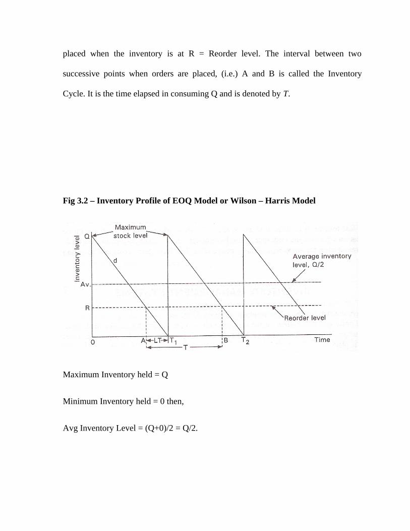
placed when the inventory is at R = Reorder level. The interval between two
successive points when orders are placed, (i.e.) A and B is called the Inventory
Cycle. It is the time elapsed in consuming Q and is denoted by T.
Fig 3.2 – Inventory Profile of EOQ Model or Wilson – Harris Model
Maximum Inventory held = Q
Minimum Inventory held = 0 then,
Avg Inventory Level = (Q+0)/2 = Q/2.

As per the assumptions, the purchase price of the units is uniform, no need for
safety stocks, decisions as to when to order and quantity to order are known. So, we
consider only the ordering cost and the holding cost.
Let Q = Ordering Quantity
O (Q) = Total annual ordering cost
H (Q) = Total annual holding cost
T (Q) = Total (Variable) Annual Inventory Cost.
Therefore, T (Q) = O (Q) + H (Q)
If N = No of times an order is placed in a year
C0 = Ordering cost per order
Then O(Q) = NC0
If annual demand = D and order quantity = Q,
then N = Orders in a year =D/Q
and O(Q) = (DC0)/Q
If Ch = Unit Holding cost (in Rupees per unit per year)
and Q/2 = Average Inventory Held, then H(Q) = (QCh)/2
Therefore, T(Q) = {(DC0)/Q} + {(QCh)/2}
To find the value of Q corresponding to the lowest value of T (Q) we find the
derivative and equate it to Zero.
d /d (Q) of {T (Q)} = d /d(Q) of {(DC0)/Q} + {(QCh)/2} = 0

Solving we get - (DC0)/Q2 = Ch/2
=> Q = [(2DC0)/Ch]1/2 = Q* = Economic Order Quantity or EOQ
To verify that this point is the minimum point, the second derivative > 0.
Here d2/d (Q) of {T (Q)} = [(2DC0)/Q3] which is a value > 0.
If T (Q*) = Minimum Annual Inventory Cost
Then T (Q*) = {(DC0)/Q*} + {(Q*Ch)/2}
Substituting Q* = [(2DC0)/Ch]1/2 in the above equation, we get
T (Q*) = [2DC0Ch]1/2
From the above explanations,
T* = Q*/D and
N* = 1/ T* = D/ Q*
Where T*= Optimal Interval between successive orders = Inventory Cycle Time
N*= Optimal number of orders placed in a year.
b) EOQ Model with Price Breaks
In real life, the assumption that unit costs of the item under consideration is
uniform may not be practical. Price discounts are based on the quantity for which
orders are placed. Lower rates for larger orders are quoted and one or more price
breaks may be offered by the seller. If unit cost price was uniform, then the
purchasing cost of the item was irrelevant as far as the cost model to determine EOQ
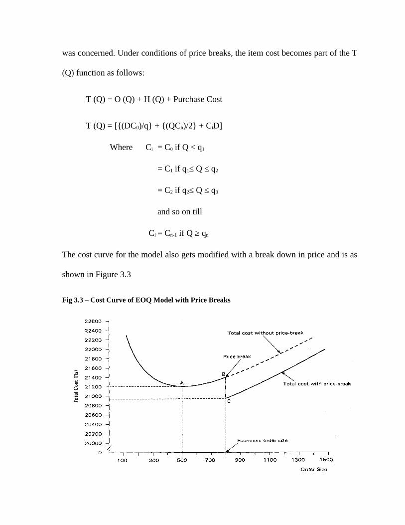
was concerned. Under conditions of price breaks, the item cost becomes part of the T
(Q) function as follows:
T (Q) = O (Q) + H (Q) + Purchase Cost
T (Q) = [{(DC0)/q} + {(QCh)/2} + CiD]
Where Ci = C0 if Q < q1
= C1 if q1≤ Q ≤ q2
= C2 if q2≤ Q ≤ q3
and so on till
Ci = Cn-1 if Q ≥ qn
The cost curve for the model also gets modified with a break down in price and is as
shown in Figure 3.3
Fig 3.3 – Cost Curve of EOQ Model with Price Breaks

c) EOQ Model for Production Runs or The Build-Up Model
Here, the goods are received for inventory at a constant rate over time and
they are also being consumed at a constant rate. This is relevant for situations when
items are produced internally in the factory and not bought from suppliers. Inventory
builds up when the rate at which the items are produced is higher than the rate of
their usage or depletion and is shown in Figure 3.4.
Fig 3.4 – Inventory Profile of Build Up Model or EOQ Model for Production Run
Here, the total order quantity Q is produced over a period tp and is defined by
the production rate, p. The average inventory level is determined not only by the lot
size Q, but also by the production rate, p and depletion rate, d.
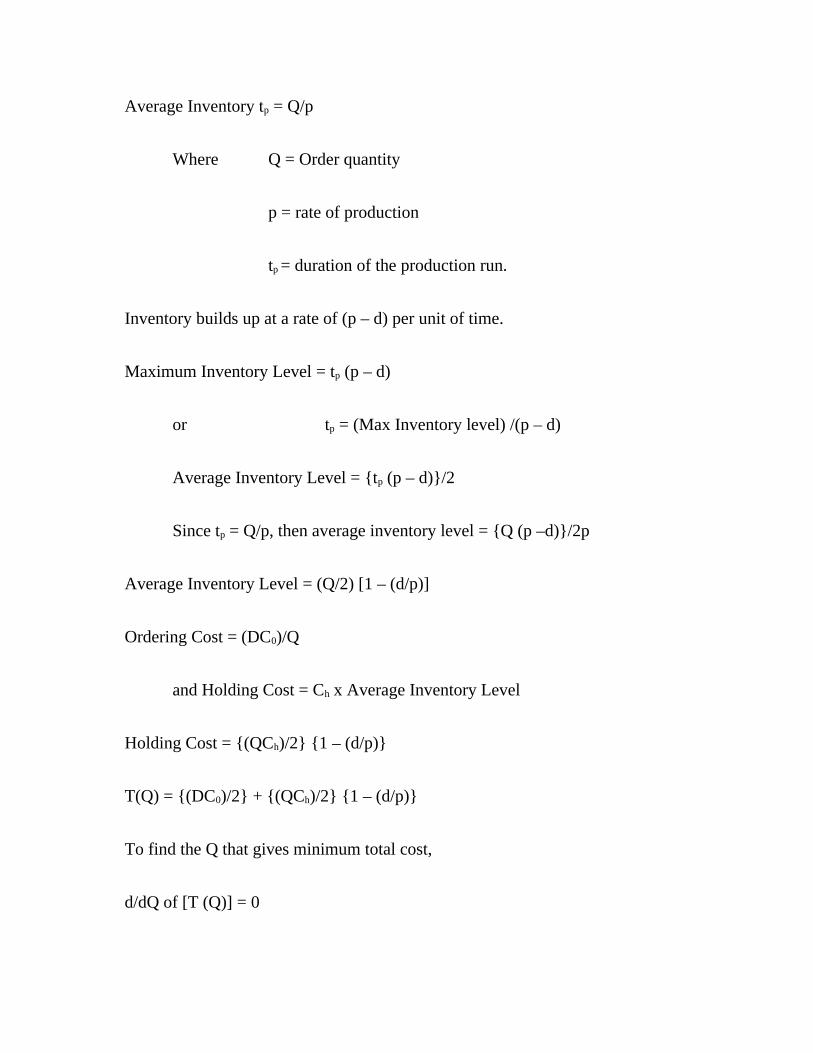
Average Inventory tp = Q/p
Where Q = Order quantity
p = rate of production
tp = duration of the production run.
Inventory builds up at a rate of (p – d) per unit of time.
Maximum Inventory Level = tp (p – d)
or tp = (Max Inventory level) /(p – d)
Average Inventory Level = {tp (p – d)}/2
Since tp = Q/p, then average inventory level = {Q (p –d)}/2p
Average Inventory Level = (Q/2) [1 – (d/p)]
Ordering Cost = (DC0)/Q
and Holding Cost = Ch x Average Inventory Level
Holding Cost = {(QCh)/2} {1 – (d/p)}
T(Q) = {(DC0)/2} + {(QCh)/2} {1 – (d/p)}
To find the Q that gives minimum total cost,
d/dQ of [T (Q)] = 0
[d/dQ of {(DC0)/2}] + [d/dQ of {(QCh)/2} {1 – (d/p)}] = 0
Solving we get
Q = Q* = EOQ = [{2DC0/Ch}]1/2 x [{p/(p –d)}]1/2
T (Q*) = [{2DC0Ch}]1/2 x [{(p –d)/p}]1/2
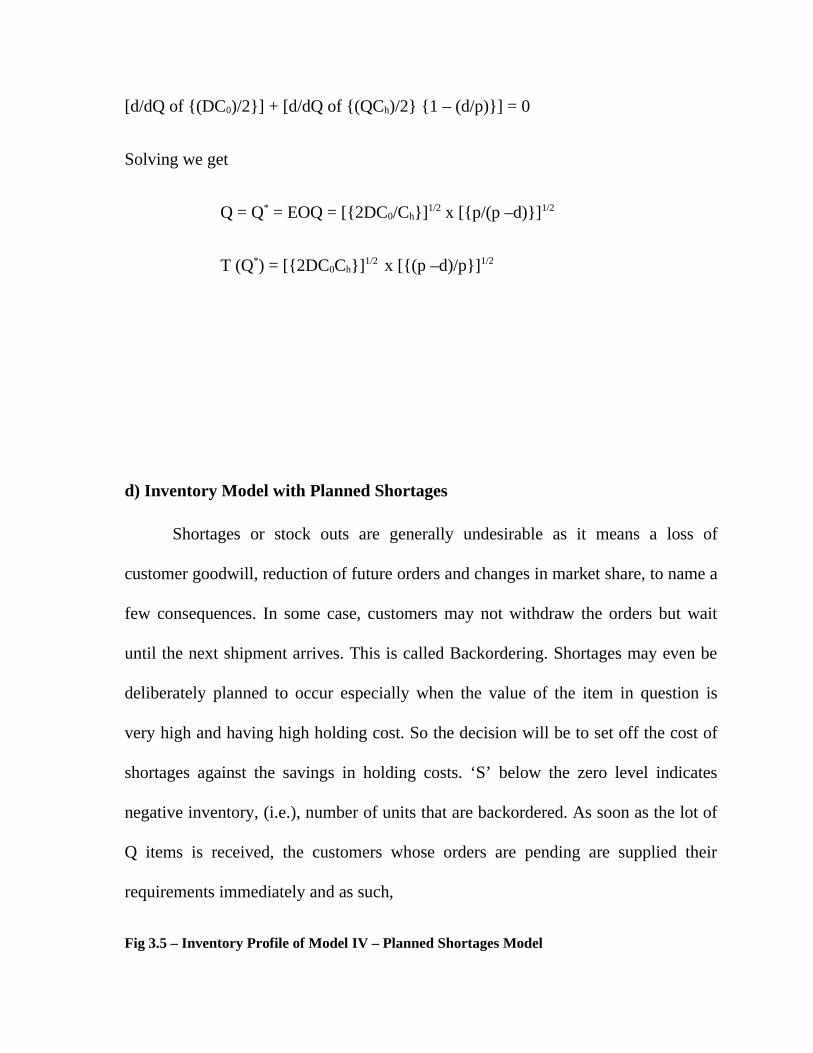
d) Inventory Model with Planned Shortages
Shortages or stock outs are generally undesirable as it means a loss of
customer goodwill, reduction of future orders and changes in market share, to name a
few consequences. In some case, customers may not withdraw the orders but wait
until the next shipment arrives. This is called Backordering. Shortages may even be
deliberately planned to occur especially when the value of the item in question is
very high and having high holding cost. So the decision will be to set off the cost of
shortages against the savings in holding costs. ‘S’ below the zero level indicates
negative inventory, (i.e.), number of units that are backordered. As soon as the lot of
Q items is received, the customers whose orders are pending are supplied their
requirements immediately and as such,
Fig 3.5 – Inventory Profile of Model IV – Planned Shortages Model

Maximum Inventory Level = (Q – S)
Inventory Cycle T is divided into two phases
t1 = Time when inventory is on hand and orders are filled as and when
they occur.
t2 = Time when it is a stock out situation and orders are placed
as Back orders.
T (Q) = O (Q) + H (Q) + S (Q) where S (Q) = Annual Shortage cost.
From the figure,
O (Q) = (DC0)/Q =>Annual Ordering Cost
H (Q) = {(Q – S)/2}Cht1 during a cycle
(Q – S) is sufficient to last a period t1
(Q – S) = t1d => From the Figure
where d = Usage rate
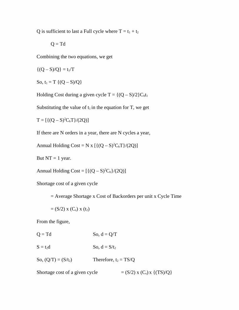
Q is sufficient to last a Full cycle where T = t1 + t2
Q = Td
Combining the two equations, we get
{(Q – S)/Q} = t1/T
So, t1 = T {(Q – S)/Q}
Holding Cost during a given cycle T = {(Q – S)/2}Cht1
Substituting the value of t1 in the equation for T, we get
T = [{(Q – S)2ChT}/(2Q)]
If there are N orders in a year, there are N cycles a year,
Annual Holding Cost = N x [{(Q – S)2ChT}/(2Q)]
But NT = 1 year.
Annual Holding Cost = [{(Q – S)2Ch}/(2Q)]
Shortage cost of a given cycle
= Average Shortage x Cost of Backorders per unit x Cycle Time
= (S/2) x (Cs) x (t2)
From the figure,
Q = Td So, d = Q/T
S = t2d So, d = S/t2
So, (Q/T) = (S/t2) Therefore, t2 = TS/Q
Shortage cost of a given cycle = (S/2) x (Cs) x {(TS)/Q}
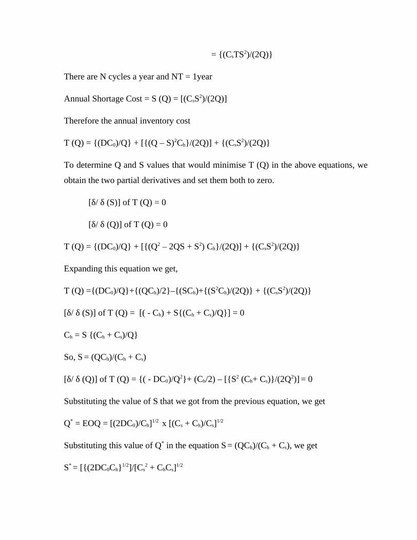
= {(CsTS2)/(2Q)}
There are N cycles a year and NT = 1year
Annual Shortage Cost = S (Q) = [(CsS2)/(2Q)]
Therefore the annual inventory cost
T (Q) = {(DC0)/Q} + [{(Q – S)2Ch}/(2Q)] + {(CsS2)/(2Q)}
To determine Q and S values that would minimise T (Q) in the above equations, we
obtain the two partial derivatives and set them both to zero.
[δ/ δ (S)] of T (Q) = 0
[δ/ δ (Q)] of T (Q) = 0
T (Q) = {(DC0)/Q} + [{(Q2 – 2QS + S2) Ch}/(2Q)] + {(CsS2)/(2Q)}
Expanding this equation we get,
T (Q) ={(DC0)/Q}+{(QCh)/2}–{(SCh)+{(S2Ch)/(2Q)} + {(CsS2)/(2Q)}
[δ/ δ (S)] of T (Q) = [( - Ch) + S{(Ch + Cs)/Q}] = 0
Ch = S {(Ch + Cs)/Q}
So, S = (QCh)/(Ch + Cs)
[δ/ δ (Q)] of T (Q) = {( - DC0)/Q2}+ (Ch/2) – [{S2 (Ch+ Cs)}/(2Q2)] = 0
Substituting the value of S that we got from the previous equation, we get
Q* = EOQ = [(2DC0)/Ch]1/2 x [(Cs + Ch)/Cs]1/2
Substituting this value of Q* in the equation S = (QCh)/(Ch + Cs), we get
S* = [{(2DC0Ch}1/2]/[Cs2 + ChCs]1/2

Substituting these two values in the original T(Q) equation we get
T (Q) = [{(2DC0Ch}1/2] x [(Cs)/(Cs + Ch)]1/2
Besides these deterministic models, there are also a number of probabilistic
models available with parameters like Safety Stock and Service Level included in the
analysis. It is on the basis of these models that the current literature on inventory
management and control has been formalised.
Even though the theoretical models of inventory are all linear in nature, in
reality, the inventory models do not always follow linearity. An example of a realistic
inventory profile is shown in Figure 3.6.
In a realistic inventory model, the demand is not continuous and uniform. It is
discrete and irregular. In the above figure, four cycles are displayed. In the first cycle,
the demand during lead-time (DDLT) is more than the expected demand, but there is
sufficient safety stock (SS) to meet the demand. In the second cycle, the demand is so
great that the amount of SS cannot meet it and this results in a stock-out situation.
The third cycle is a condition where the DDLT is less than the expected demand. The
fourth cycle illustrates a situation where the DDLT just matches the expected
demand. Even when the demand is irregular and unequal, the amount of average
stock held would be nearly (Q/2 + SS). Notice that the DDLT would be sometimes
more and sometimes less that the expected demand. Therefore, an amount equal to
the SS would nearly always be carried. The idea of keeping safety stock is clearly to
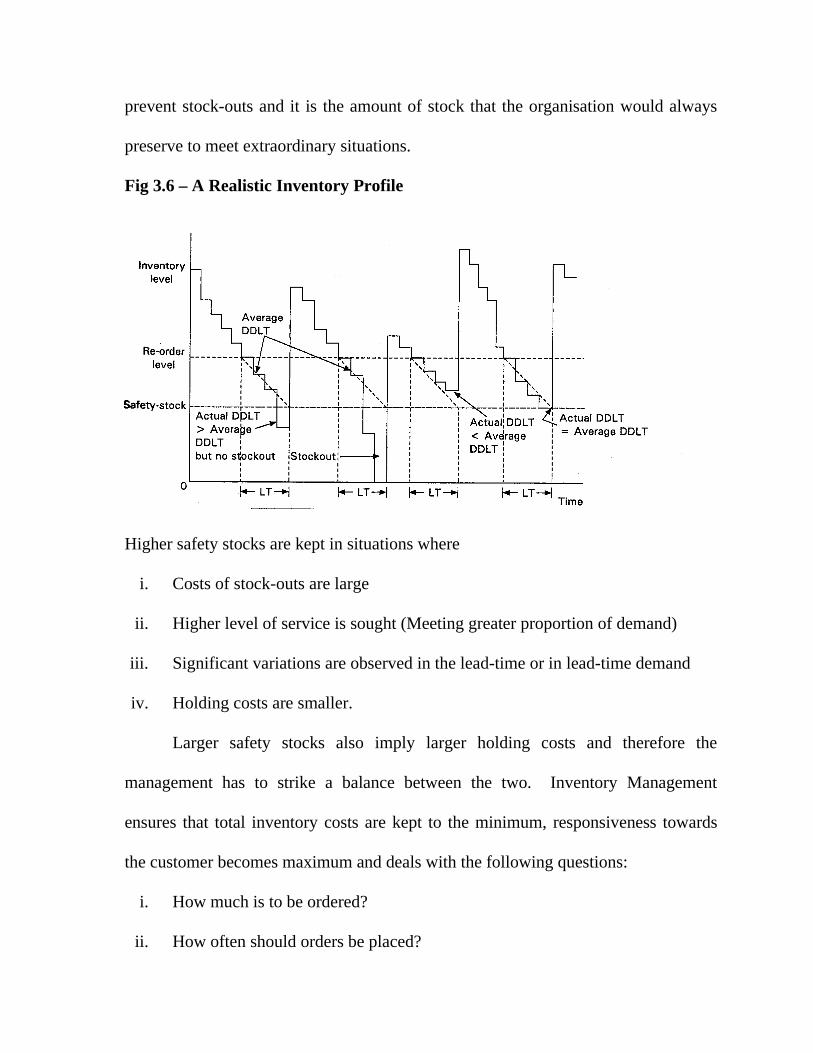
prevent stock-outs and it is the amount of stock that the organisation would always
preserve to meet extraordinary situations.
Fig 3.6 – A Realistic Inventory Profile
Higher safety stocks are kept in situations where
i. Costs of stock-outs are large
ii. Higher level of service is sought (Meeting greater proportion of demand)
iii. Significant variations are observed in the lead-time or in lead-time demand
iv. Holding costs are smaller.
Larger safety stocks also imply larger holding costs and therefore the
management has to strike a balance between the two. Inventory Management
ensures that total inventory costs are kept to the minimum, responsiveness towards
the customer becomes maximum and deals with the following questions:
i. How much is to be ordered?
ii. How often should orders be placed?

iii. When should the order be placed?
iv. How much stock is to be kept as Safety Stock?
The accuracy of the decisions on Inventory Management is directly
proportional to the accuracy of the forecasting methods used and the relevance of the
data that is received about the consumer demand. Hence, information plays a big role
in proper management of inventories. The company’s performance is judged on the
basis of its efficiency of operations and its responsiveness to the consumer.
To ensure that the best returns are achieved on capital and other factors of
production invested in the stock, a balance should be struck between balancing the
service levels with the cost of providing a particular level of service through proper
inventory control. The obvious solution to problems concerning level of service and
responsiveness is to increase the stock levels. This will reduce back-orders, out-of-
stock situations, lead-times and an increase in customer service. Maintaining higher
levels of stock increases the related costs of carrying inventory, insurance, taxes,
obsolescence, warehousing and materials handling. Even though lower stocks reduce
the costs of inventory, lack of readily available products on demand can mar the
goodwill of the organisation.
Kapoor and Kansal (2003) define Inventory control as a set of policies and
procedures by which an organisation determines which materials it will hold in the
stock and the quantity each one of them it will carry. Efforts are made to keep the
safety stock at the lowest level possible. It is also kept proportional to the uncertainty
or risk level. Selective Inventory Control is a methodology based on the concept of
80-20 used in Welfare Economics by a German Economist, Pareto.
Using the same principle, one can find that 20% of total stock contributes to
80% of the value. This 20% of total stock is crucial to the companies as far as
production is concerned. In selective control, inventory of high value items is
controlled because they contribute to give highest returns. Lesser care is assigned for
low value items, as returns are low.
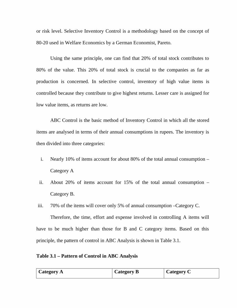
ABC Control is the basic method of Inventory Control in which all the stored
items are analysed in terms of their annual consumptions in rupees. The inventory is
then divided into three categories:
i. Nearly 10% of items account for about 80% of the total annual consumption –
Category A
ii. About 20% of items account for 15% of the total annual consumption –
Category B.
iii. 70% of the items will cover only 5% of annual consumption –Category C.
Therefore, the time, effort and expense involved in controlling A items will
have to be much higher than those for B and C category items. Based on this
principle, the pattern of control in ABC Analysis is shown in Table 3.1.
Table 3.1 – Pattern of Control in ABC Analysis
Category A Category B Category C
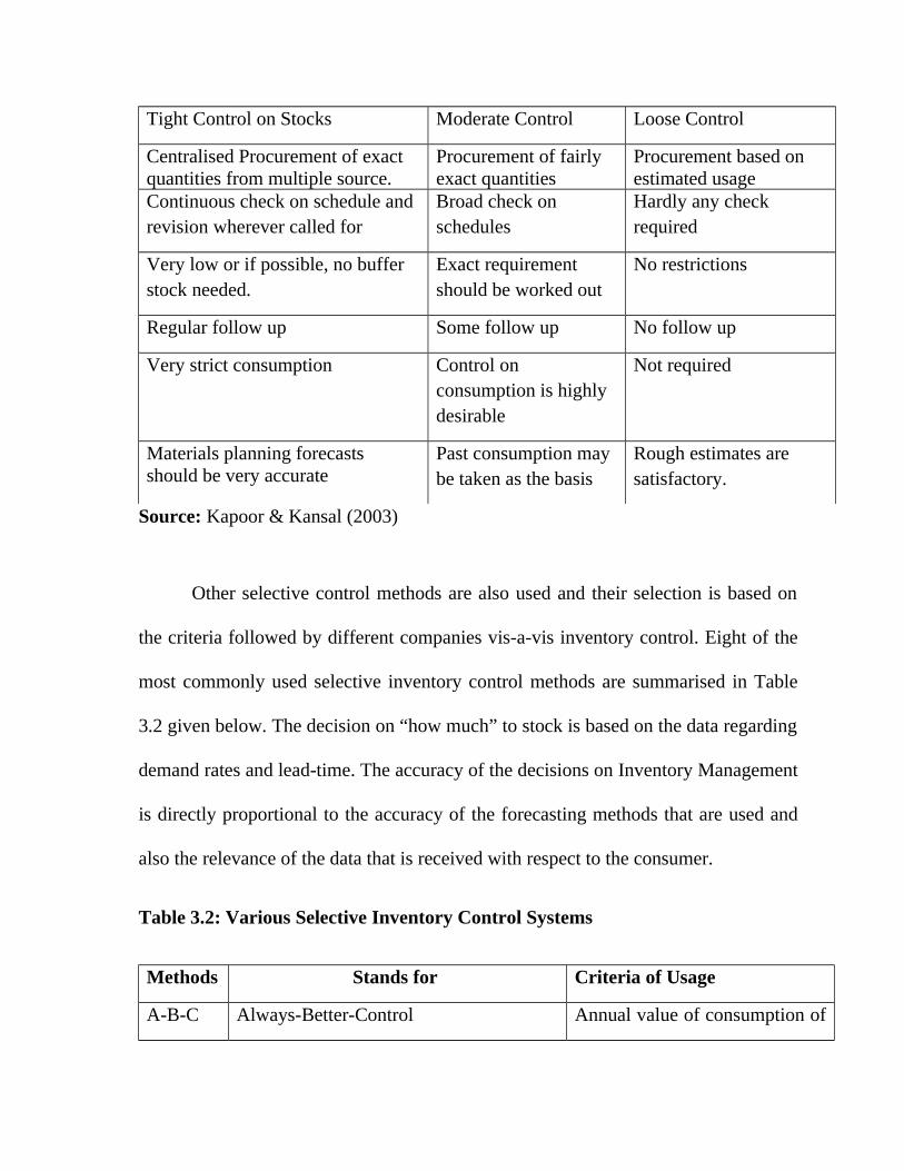
Tight Control on Stocks Moderate Control Loose Control
Centralised Procurement of exact quantities from multiple source.
Procurement of fairly exact quantities
Procurement based on estimated usage
Continuous check on schedule and revision wherever called for
Broad check on schedules
Hardly any check required
Very low or if possible, no buffer stock needed.
Exact requirement should be worked out
No restrictions
Regular follow up Some follow up No follow up
Very strict consumption Control on consumption is highly desirable
Not required
Materials planning forecasts should be very accurate
Past consumption may be taken as the basis
Rough estimates are satisfactory.
Source: Kapoor & Kansal (2003)
Other selective control methods are also used and their selection is based on
the criteria followed by different companies vis-a-vis inventory control. Eight of the
most commonly used selective inventory control methods are summarised in Table
3.2 given below. The decision on “how much” to stock is based on the data regarding
demand rates and lead-time. The accuracy of the decisions on Inventory Management
is directly proportional to the accuracy of the forecasting methods that are used and
also the relevance of the data that is received with respect to the consumer.
Table 3.2: Various Selective Inventory Control Systems
Methods Stands for Criteria of Usage
A-B-C Always-Better-Control Annual value of consumption of
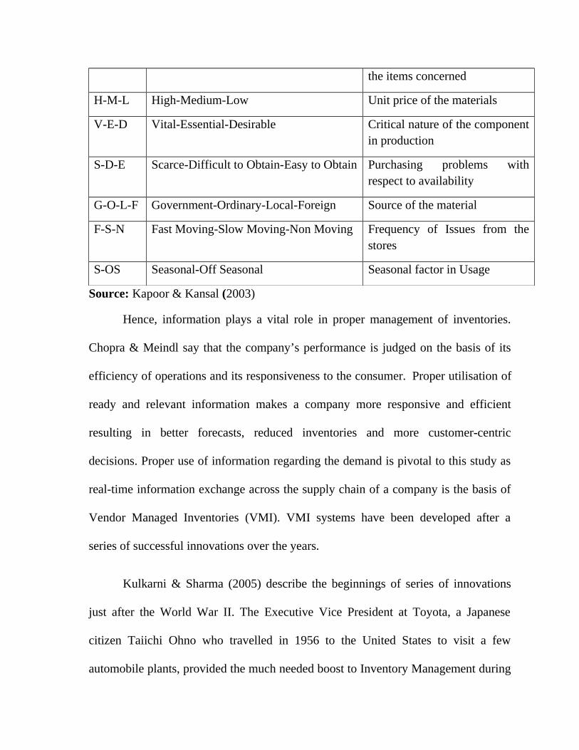
the items concerned
H-M-L High-Medium-Low Unit price of the materials
V-E-D Vital-Essential-Desirable Critical nature of the component in production
S-D-E Scarce-Difficult to Obtain-Easy to Obtain Purchasing problems with respect to availability
G-O-L-F Government-Ordinary-Local-Foreign Source of the material
F-S-N Fast Moving-Slow Moving-Non Moving Frequency of Issues from the stores
S-OS Seasonal-Off Seasonal Seasonal factor in Usage
Source: Kapoor & Kansal (2003)
Hence, information plays a vital role in proper management of inventories.
Chopra & Meindl say that the company’s performance is judged on the basis of its
efficiency of operations and its responsiveness to the consumer. Proper utilisation of
ready and relevant information makes a company more responsive and efficient
resulting in better forecasts, reduced inventories and more customer-centric
decisions. Proper use of information regarding the demand is pivotal to this study as
real-time information exchange across the supply chain of a company is the basis of
Vendor Managed Inventories (VMI). VMI systems have been developed after a
series of successful innovations over the years.
Kulkarni & Sharma (2005) describe the beginnings of series of innovations
just after the World War II. The Executive Vice President at Toyota, a Japanese
citizen Taiichi Ohno who travelled in 1956 to the United States to visit a few
automobile plants, provided the much needed boost to Inventory Management during

the middle of the 20th century. The ‘Supermarkets’ in America caught his eye. Ohno
was amazed by the way in which shoppers selected ‘what’ and ‘how much’ they
wanted all by themselves. Later this materialised into a ‘Pull System’ at Toyota, in
which each production line became a ‘supermarket’ for the next in line. Each line
would make available only the item that the next line wanted and nothing more. This
was possible by the kanban (sign board) system which indicates to the preceding
stage what the next stage wanted as replenishment of components and subassemblies.
This was improved upon by the kaizen system (continuous improvement),
made famous by Masaaki Imai, which stressed on making the right item the first
time. The Japanese even invented machines that shut down as soon as an error in
production is detected so that defective items do not pile up. All these were done with
the intention of reduction of costs due to bad production practices.
Defects were detected using a Cause-Effect Diagram called Ishikawa diagram
(after its creator, Kaoru Ishikawa) or the fishbone diagram, which was a pictorial
display of the possible causes of problems, their origin and the possible replacement
strategies.
During this time, the quality expert, W. Edwards Deming was in Japan
conducting Statistical Quality Control programmes at their production plants. He was
instrumental in popularising the Total Quality Management (TQM) philosophy
among the Japanese. TQM encompassed every aspect of the management of a
company and quality control was not practiced just on the shop floor, but also in the
administrative offices. In time, by the 1970s, Japanese products flooded the
American markets and a glaring difference in the quality as well as cost of goods was
noted. Americans too started replicating the Japanese success story and the Japanese
production system of kanban-kaizan-ishikawa was repackaged for the developed
world as Just-In-Time (JIT) Production in the later years.
Also known as Lean or Stockless production, JIT aims at eliminating sources
of manufacturing waste by producing the right component at the right place at the
right time. An attempt is made to work towards the goal of achieving the “ideal lot
size of one unit” and “a queue size of zero.” As a cushion against possible problems,
underutilised capacity of the plant is used whenever an excess requirement arises
instead of blocking capital in buffer inventory. This results in an improvement of
product quality and a significant reduction in delivery lead-time, breakdowns and
other costs of machine set-up.
A uniform load is given to all work centres through constant daily, repetitive
production. Single digit set-up times are aimed at through better planning, product &
process redesign. Suppliers encourage more frequent deliveries so that economic lot
sizes can be manufactured and inventory kept to a minimum. Production lead-time is
also kept to a minimum by reducing queue length, moving workstations closer,
application of group & cellular layout.
To cut down on unnecessary transportation costs, suppliers are encouraged to
relocate closer to the factory. Preventive maintenance schedules are followed to

avoid machine idle time. Job rotation and cross training are practiced by the work
force so that there is a smooth substitution in case of absenteeism. Workers are given
more responsibility for the quality of the work they do so that they can stop work
whenever a defect is observed. This was called the 'Jidoka’ programme.
Supplier quality assurance is stressed upon and a zero defect programme
implemented. Techniques like ‘JIT Lights’ were used to indicate slow work and
stoppages. The Kanban system of using cards & bins to convey parts between
workstations in small quantities (ideally, one unit) were used, though it is not
compulsory for a JIT programme. A Kanban programme, on the other hand can be
implemented only when JIT is being used.
Cudmore (2003) describes a method called Postponement as being based on
the principle of seeking to design products using common components, platforms or
modules but in which the final assembly takes place only when the final market
destination or customer requirement is known. To have full advantage of the system,
products and processes are designed and engineered in a way that semi-finished
products can be assembled and configured to provide high levels of variety.
Inventory is held only at the generic level and not at the finished goods level. Mass
customisation is possible. There is high flexibility and forecasting at the generic level
is easier.
Flexible Manufacturing Systems or FMS tried to meet the customer
requirement of additional variety of products in shorter and shorter time frames. This
brought about a fundamental shift away from economies of scale to economies of
scope, (i.e.), smaller quantities of a wider range of products. A minimum quantity of
every variant of a product is produced daily so that a minimum stock of every item is
always available. The machines are also so designed that they can be reconfigured
within no time to make the next product. This is practiced by Dell Computers who
are the world’s largest custom-built PC manufacturers. It achieves a strategic fit with
their competitive strategy of providing any configuration asked by the customer in a
few days time. This ensured that very few inventories were kept in stock.
The concept of JIT has transformed the world of Logistics. To make a
company responsive and efficient, a responsive and efficient logistical support is
imperative. It is to ensure that the demand is captured real-time and the right product
is delivered at the right place at the right time. This led to companies using new
concepts in logistics like 3PL (Third Party Logistics) and 4PL (Fourth Party
Logistics).
3PL involves a specialised logistics service provider who has entered into a
contract for a given period with the supplier or shipper. Kulkarni and Sharma (2005)
say that they provide transport, warehousing, freight payment and audit, inventory
and value added services like reengineering of the supply chain with respect to
logistics. Several multinationals like Fed Ex, UPS, and DHL Express are 3PL players.
A 4PL provider is a supply chain integrator that assembles and manages the
resources, capabilities and technology of its own organisation and that of

complementary service providers to deliver a comprehensive supply chain solution. It
is a combination of management consulting and 3PL.
JIT tried to eliminate inventory and allowed buyers and suppliers to have a
coordinated work environment. JIT II or Lance Dixon Bose Configuration was a
modification on JIT which helped to eliminate the buyer and salesman. It empowered
the supplier to post an employee inside the buyer’s production facility and write his
own purchase order, thus giving complete freedom to the supplier to make key
decisions about the supplied product. This was the pre-cursor to the now popular
Vendor Managed Inventory (VMI) system.
3.6 Vendor Managed Inventory
The American Production and Inventory Control Society defines Vendor
Managed Inventory (VMI) as a means of optimising supply chain performance in
which the supplier has access to the customer’s inventory data and is responsible for
maintaining the inventory level required by the customer. It is accomplished by a
process in which re-supply is done by the vendor through regularly scheduled
reviews of on-site inventory.
VMI is the first approach that allows information to be used more
intelligently. This concept is finding its applicability in automobile, apparel and retail
sectors mainly due to the advancements in the field of information technology with
broader bandwidth and gadgets like Bar Code Scanners, Electronic Point of Sales
(EPOS) data capture equipments, Electronic Data Interchange (EDI), Radio
Frequency Identification Devices (RFID) and mainly the Internet. Over the last two
decades, we can clearly see a slow transition in the power of managing a supply
chain shifting from the retailer to the vendor. Chopra et al (2000) calls it as a change
of convenience.
VMI is referred in many ways based on sector of application, ownership
issues and scope of implementation. Lee et al (2000) termed it Quick Response (QR).
Cachon & Fisher (1997) referred to it as Synchronized Consumer Response (SCR),
Continuous Replenishment (CR) or Efficient Consumer Response (ECR). Holmstrom
et al (2000) referred to it as Rapid Replenishment (RR) and Collaborative Planning,
Forecasting and Replenishment (CPFR).
The concept of VMI evolved mainly due to the rising costs experienced
through the supply chain. The errors inherent in the forecasting methods used in a
supply chain will manifest itself in every subsequent process along the chain. This
results in inventories that are either above or below the required levels, both of which
can prove to be dangerous to the company in the long run.
3.7 Bullwhip Effect
The term “bullwhip effect” coined by Lee et al. (1997a,b) refers to an
economic condition relating to materials and product supply and demand. The
bullwhip effect creates large swings in demand on the supply chain resulting from
relatively small but unplanned variations in consumer demand that escalates with
each link in the supply chain. It is a situation where the information about the final
customer's actual demand is distorted from one end of the supply chain to the other.
The errors in demand forecasting causes the Bullwhip Effect (Lee &
Padmanabhan, 1997) which is a phenomenon due to which the size of the inventory
‘shortages’ or ‘excesses’ rise, the further a firm is from the final consumer in a
supply chain. The time lags together with use of batch orders from the buyers
amplifies demand fluctuations as they go up the supply chain and makes the demand
variations more at the supplier’s end than at the buyer’s end.
A bullwhip has a structure where the end that hits the bull is thin (analogous to
actual demand) and the handle of the whip which is held is much thicker than the
cracking end (analogous to the wrongly forecasted demand which is much higher
than the actual demand). Events that trigger the bullwhip effect include increases or
decreases in order frequency and order quantities, batching of orders to reduce the
shipping costs, price reductions or sales quotas as part of sales promotions at the
store, return and refund policies, all of which can create differences between
forecasted figures and actual consumer demand. These triggers can happen at any
point in the supply chain – consumer, retailer, distributor, manufacturer or raw
material supplier. A slight variation at one link gets amplified as the order moves up
the supply chain.

Each level visualizes a greater demand than it actually seeks to fulfil. Once the
amplified need reaches the top of the supply chain, an oscillation is triggered, which
swings the supply and demand variables in the opposite direction. This triggers an
oversupply that drives down demand, with the net result being excess inventory
storage costs, excess inventory procurement costs, lost profits, and substandard
service at each level.
Variations also happen due to uncontrollable reasons like weather, natural
disasters, industrial accidents and fires, strikes, changes in the tax rates and other
political reasons. A recent example can be cited where the Toyota Production System
famed for its Just In Time production ran into rough weather globally due to the
Japanese earthquake and tsunami resulting in demand-supply variations all over the
world, thus necessitating production to be run from places like India, to meet the
variation in demand.
Farther the supply chain partner from the final consumer, more distorted and
amplified is the error in the forecast. Lee et al. (1997a,b) identified that there are five
causes of bullwhip - non-zero lead-times, demand signalling processing, price
variations due to promotions, rationing & gaming and order batching.
The traditional supply chain is a system where each supply chain partner bases
the production or delivery orders solely on the basis of sales to the customer,
inventory levels and at times work-in progress (WIP) targets. Each stage in the
supply chain has information only on what the customers prefer and not on which
products the end customer will actually buy on that day. This lack of visibility of real
demand leads to a lot of guessing which in turn causes problems in the supply chain
if it is not properly designed. This situation is called the Forrester effect.
Houlihan effect is also called rationing effect. As shortages or missed
deliveries occur in the traditional supply chain, customers overload their orders,
leading to bullwhip effect. Some organizations resort to batch ordering to achieve
economies of scale but this can lead to bullwhip effect as actual requirements are not
reconciled. The error in forecasts caused through batch ordering is called Burbridge
effect.
Industrial engineers and economists have over the years tried to reduce
inventories at each stage along the supply chain by capturing the demand position at
each stage more accurately than before. This results in better forecasting and
operational efficiencies and this is achieved through proper management of the four
supply chain drivers – facilities, transport, inventory and information.
To save the costs of financing inventory, companies at times enter into VMI
arrangements just to force their suppliers to manage inventory for the entire supply
chain and shift this cost to them. It was observed in many cases that suppliers simply
took ownership of the inventory without major changes in the management styles.
Holding this inventory increased supplier’s costs and they had to raise their prices
which resulted in no real reduction in costs to the subsequent supply chain members,
as they merely shifted costs back and forth the supply chain.
As Chopra et al (2000) mentioned, attempts to optimise the performance by
the individual links in the supply chain results in the sub-optimisation of the overall
supply chain. Cost reduction can be achieved only if the inventory carried is
positioned in the supply chain at a point where the supply chain effectiveness is
maximised.
Most literature like Lee & Padmanabhan (1997a & 1997b) show that the
unwanted Bull Whip effect can be reduced through advanced information sharing
through the supply chain, which in turn leads to lower inventory levels and better
supply chain performances. Lin and Shao (2000) have found that the sharing of
information in a retailer-supplier partnership is critical to both the parties. Cooray
and Ranatunga (2001) studied the power relationships between the retailer and
supplier and found out a cultural angle to it.
Over the decades, the companies that have implemented VMI have seen more
accurate transfers of information across the supply chain due to the advancements in
Information Technology (IT), Radio Frequency Identification Devices (RFID),
Barcode readers & scanners and Electronic Data Interchange (EDI). This has led to
the capture of demand information as close to the consumer as possible and in very
accurate forecasts. This in turn has reduced the inventory levels throughout the
supply chain.
A typical VMI programme involves a supplier who monitors inventory levels
at the customer’s warehouses using information sharing technology and assumes the
responsibilities of tracking and replenishing that inventory. Aparajit (2005) says that
the basic objective of VMI is to give the manufacturer access to Point of Sales (POS)
information to set the replenishment activity closer to actual sale and also to give the
manufacturer a demand-centric view of replenishment and production planning.
VMI is a backward replenishment programme that uses the exchange of
information between the retailer and the supplier to allow the supplier to manage and
replenish the merchandise at the store or warehouse level. The buyer is charged for
the material only when it is used, so the vendor incurs the carrying cost of stocking
the material in the customer’s facility. The purchase orders are created on the basis
of the demand information exchanged by the retailer/customer. This makes the
manufacturer more customer-centric as the demand data is captured closer to real
time. This also provides improved visibility of information across the supply chain
pipeline and results in fewer stock-outs and greater cost reductions.
In a VMI system, the onus of forecasting and inventory management shifts to
the vendor/supplier/manufacturer (V/S/M) and is not with the
retailer/distributor/customer (R/D/C). EDI is to be established and EPOS systems
have to be set up so that real time sales and inventory data is transferred to the
V/S/M. The supplier creates purchase orders based on the inventory data and fill
rates. Fill rates are the proportion of customer demand that can be satisfied from the
available inventory. The vendor creates and maintains the inventory stock plan for
the retailer. The vendor sends the Advance Shipping Notices before the product is
sent to the retailer’s warehouse. Then, the vendor follows this up with an Invoice to
the retailer. On receipt of the product or consignment, the retailer does invoice
matching and handles the payment. Kumar & Kumar (2001) has illustrated this as
shown in Figure 3.7.
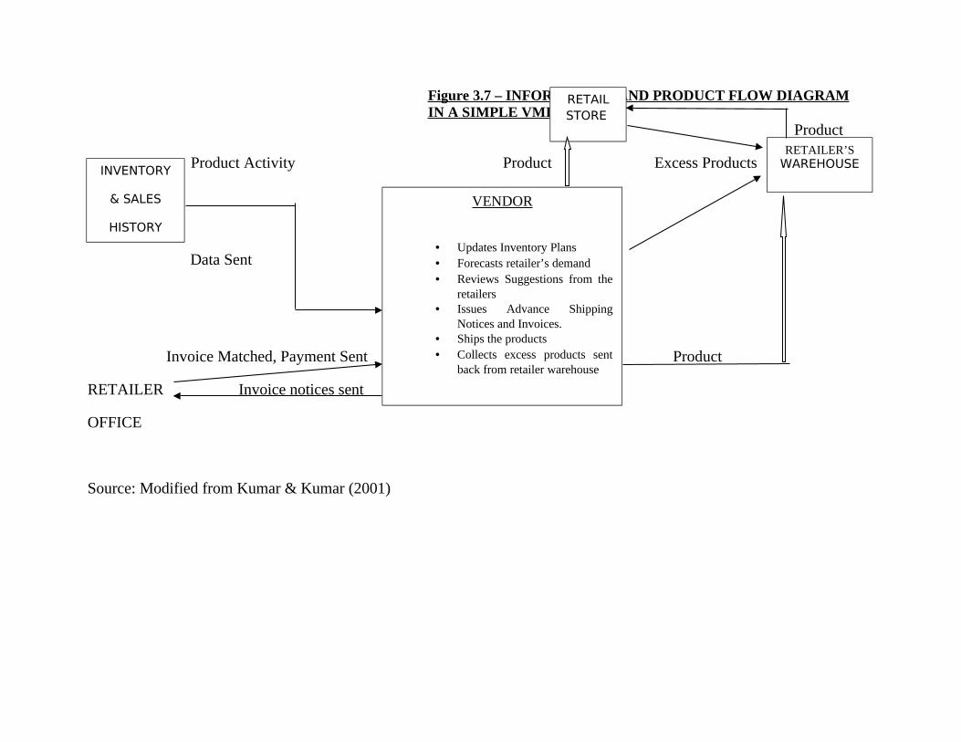
Figure 3.7 – INFORMATION AND PRODUCT FLOW DIAGRAMIN A SIMPLE VMI MODEL
Product
Product Activity Product Excess Products
Data Sent
Invoice Matched, Payment Sent Product
RETAILER Invoice notices sent
OFFICE
Source: Modified from Kumar & Kumar (2001)
INVENTORY
& SALES
HISTORY
RETAIL STORE
RETAILER’SWAREHOUSE
VENDOR
• Updates Inventory Plans• Forecasts retailer’s demand• Reviews Suggestions from the
retailers• Issues Advance Shipping
Notices and Invoices.• Ships the products • Collects excess products sent
back from retailer warehouse
Since VMI uses automatic electronic messages to keep track of the current stock
situation and planned sales forecasts, it also leads to improved inventory turnovers
and lower safety stock. It has been found that ever since Wal-Mart took up the VMI
initiative, the textile industry also has adapted VMI into their operations. Ironically,
the industries that face complex situations are among the last to adopt this.
Supermarkets and malls haves also started adopting this though a little late than
expected. Auto component manufacturers in India have taken this up in earnest too.
A very high level of trust and confidence is necessary between the parties.
Long-term contracts are typically entered into with VMI systems. Yao et al (2005)
mentions that VMI is a collaborative venture that authorises the suppliers to manage
the buyer’s inventory of stock-keeping units (SKU). Customers or retailers no longer
place orders, but instead only share information with the vendor, who takes
responsibility for inventory management. No explicit orders are received by the
vendor, instead an indication of the upper and lower stock limits that are expected to
be kept are intimated. Within these stock-bands, it is the supplier’s responsibility to
forecast and replenish inventory.
VMI is a ‘pull’ replenishment practice which represents the highest level of
partnership where the vendor is the primary decision maker in the order placement
and inventory control processes. Simchi-Livi et al (2000) in their study mentions that
the supplier decides an appropriate inventory level for each product within previously
agreed boundaries and appropriate policies to maintain these levels.
VMI is a reality in the 21st century due to the advancements in the information
technology and telecommunications sector. High speed, high quantity data transfer is
today possible due to leased line and broadband technologies. Immediate and
elaborate data capture is also possible due to barcode scanners, EPOS (Electronic
Point of Sales) Retrieval systems and EDI (Electronic Data Interchange) devices.
Accurate tracking of any tagged device on this planet is now possible with RFID
(Radio Frequency Identification Devices) technology. Internet helps buyers share
sales and inventory information on a real time basis with suppliers, who use several
analysis software to plan production runs, scheduling deliveries, deciding
transportation routes, balancing the load of vehicles and production facilities and also
manage the order volumes and inventory at the buyer’s SKU facilities.
VMI offers the authority to that supply chain partner who has the best
visibility of the inventory position. It uses information more intelligently than in the
traditional inventory systems. VMI uses effective real time sharing of POS data
through EDI systems and analytical software tools to calculate the appropriate order
quantities, product mixes, travel routes and safety stock.
Thus VMI pushes the supply chain decision-making responsibility up the
chain. The v/s/m is in a better position to support the objectives of the entire
integrated supply chain. A wider range of customers and their demand patterns can
be observed resulting in improved forecasting. The effects of promotional

programmes and seasonal changes are automatically appended to the POS data thus
giving a better forecast.
3.8 Models of VMI
i) Authority Transfer Model
Here the inventory management cost and other activities regarding the
inventory are transferred to the vendors by the buying organisation. In its simplest
form, the supplier's representative visits the customer’s premises, to count the
inventory so as to get a picture of the replenishment requirements. Here, though the
customer gets benefits by shifting the responsibilities of inventory management to the
supplier, the whole supply chain costs remains the same. In this model, either the
costs are transferred back to the buying organisation or it eats into the operating
profits of the supplier.
ii) Joint Planning Model
This collaborative planning model consists of two stages – first being the data
sharing stage and the second takes care of forecasts and production schedules that get
jointly developed by the supply chain partners. The ‘buyer’ collaborates with the
supplier on demand and consumption details so that an agreed upon consensus
forecast of future demand is reached which favours the profits of both the companies.

iii) Fully Automated Replenishment Model
This model incorporates the positives of both the above models by aiming to
reduce total supply chain cost by focussing on costs at both buyers’ and supplier’s
premises. At the macro level, it defines the objectives and limitations of the
relationships and the power equations. At micro level, it develops the replenishment
strategy for each SKU. Once the replenishment strategy is developed, the daily
demand and the inventory level at the replenished site are closely monitored via EDI
and all strategies are based on that data.
It is this fully automated replenishment model that is currently the blueprint
for the existing VMI systems. The other two models were modified forms of JIT and
JIT II.
3.9 Global scenario of VMI
V.K. Magupu, whole-time director and Sr. Vice President, IT & Technology
Services, L & T and Chief Executive, L & T Infotech in his keynote address as Chief
Guest at the VMI Conference jointly organised by L&T Infotech and the Indian
Institute of Materials Management in Mumbai in Nov 2004 had said,
“VMI is the next big thing after Just In Time and it has tremendous
potential to create real win-win situations for both the buyer and
vendor. VMI enforces true partnerships between the buyer and vendor;
cleans up an organisation’s processes and establishes an ecosystem,
with VMI being the base motivator for improving efficiency”.
The tie-up between North America’s largest retailer, Wal-Mart and their
suppliers, Proctor & Gamble (P & G) is widely regarded as the first VMI venture. P
& G received sales data directly from the checkout counters which was used for
planning and scheduling of production and delivery to the Wal-Mart stores on a
replenishment basis.
VMI has existed much prior to EDI and other technologies. Much before the
Wal-Mart- P&G arrangement, Frito-Lays delivery trucks replenished retailer’s
shelves without going through the store owners as the involvement from the
management of the stores was found to be non-value adding for them. Even the
practice of JIT II where the supplier posts their representative at the retailer's store is
also “Vendor Managed.”
Lee & Padmanabhan (1997a, 1997b) in their path breaking research paper on
VMI have cited a number of examples worldwide to highlight the usage and results
of VMI implementation, some of which are cited below.
Wal-Mart and P&G had a VMI program together for more than ten years to
manage the inventory and production of disposable diapers, which was later extended
to other suppliers and products. Major retailers like Wal-Mart, K-Mart, Dillard
Department Stores and JC Penney, all have VMI agreements with their vendors.

Their experiences are that high volume, high turnover items are the best candidates
for VMI though it is arguable.
Chopra et al (2000) also cites a few examples in their research works. At K-
Mart, inventory turnover on seasonal items have dramatically increased to more than
10 times and for non-seasonal items to as high as 17-20 times. The customer service
levels have also risen higher than usual after VMI implementation. K-Mart has
anyway scaled back their VMI program to just 50 suppliers from an initial high of
300 confirming Dr. Chopra’s claim that VMI is best with few big vendors.
Grand Union, a New Jersey based grocery retailer with more than 100 stores
and three Distribution Centres improved inventory turnover by close to 80% and
achieved 99% service levels. Warehousing costs and out-of-stock conditions had also
decreased. Grand Union entered into VMI only with vendors who were proven
market leaders in their category and who were comfortable with technology and
supply chain innovations.
ACE Hardware, the largest hardware cooperative has also seen fill rates rise
from 4% to 96% in the past few years after VMI was introduced. Oshawa Foods, a $6
billion Canadian food distributor and retailer had VMI arrangements with Pillsbury,
Quaker and H.J.Heinz which ran into a lot of trouble initially due to hasty
implementation. Once the system was fine-tuned, customer service levels of 99%
were achieved and inventory turns multiplied 3 to 9 times.
Fred Meyer, the 131-unit chain of super centres in the Pacific Northwest
region after its VMI with two main food vendors improved service levels to 98% and
reduced inventories by 30% to 40%.
Hughes (1996) mentions that Panduit, which is one of the world’s largest
electrical component manufacturers (with about 60,000 SKUs in stock), did not see
cost savings in the VMI system in the initial stages. The company markets
exclusively through 1800 distributors in the US, who in turn sell to maintenance &
repair shops, construction firms. Profits were very less due to the heavy competition
in this field. EDI was initially used only for entering orders and not for generating
purchase order acknowledgements, advance shipping notices and invoicing all of
which were done by fax. Since all these were not integrated into a single system, the
full benefits of VMI could not materialise. Later, it developed a turnkey VMI/EDI
system called Qualified Supplier Program (QSP) created by an external vendor,
Advantis for a tailored approach specific to its industry. Panduit persuaded 34 major
suppliers to adopt QSP. Now, Panduit knows exactly what every distributor carries in
their warehouses at any point of time and automatically ships the needed items along
with generating an electronic invoice and advance shipping notice. Whenever the
customers are seen to be maintaining too much stock, Panduit generates a return
order with no restocking charges. So, they now claim to have started providing better
service and out of stock conditions are almost non-existent. This highlights that
industry specific tailoring is needed for certain systems to achieve the actual potential
of VMI.
Cataldo (1996) mentions that Motorola Inc’s semiconductor sector has a VMI
system which uses EDI to provide online visibility of a customer’s inventory and to
forecast data that provides inputs to the planning systems. Six of Motorola’s OEM
(Original Equipment Manufacturers) customers are now using this system which
allows Motorola to determine the quantity of product that a customer needs, time of
shipping and the requisite quantity. Motorola uses an auto scheduling tool known as
The Order Promising System (TOPS) and a shipment tie-up with logistics giant, UPS
called Rapid-NET in congruence with the VMI and has reduced procurement time
from an average of 23 days to 2 days for every execution cycle. Shipments are
handled exclusively by UPS and customers are given a choice to select delivery time
ranging from 1-4 days. Same rate is charged regardless of place of product origin.
Motorola prepays the freight, bills the customer as a separate invoice charge thus
reducing administrative delays.
Carbone (2005) mentions that the OEM provider, Celestica Inc., partners with
key suppliers to provide lowest cost solutions to its customers using VMI and by
stocking at locations that are close to manufacturing facilities, most of which are
outsourced to Electronics Manufacturing Service providers in China, Taiwan etc.
Michaeu (2005) mentions a case about Boeing’s Skin and Spar facility that
has a VMI relationship with Alcoa, its raw material supplier for the plant that makes

large wing products. VMI arrangement has gone a long way in solving the
forecasting and delivery problems. As a result, Boeing started sending weekly
electronic forecasts, weekly electronic inventory counts and purchase orders to
Alcoa. Alcoa in turn changed their order entry process to include the VMI agreement
and using this data for internal production. This has led to a strong and flexible
supply chain, more accurate forecasts and better production decisions.
Lenius (2005) mentions about Elkay which implemented a VMI for water
cooler and fountain products with Indianapolis based Central Supply. VMI is said to
have reduced overstock and labour related to tracking inventories there.
Sucher & McManus (2002) suggest that to streamline its supply chain
operations, Herman Miller, a leader in the industrial furniture industry, has
significantly benefited from employing a supply centre for components, managed by
the component suppliers.
All over the world, VMI is popular among raw material and component
suppliers to electronics industry, electrical sector, construction & aviation industry
and automobile giants. Retailing, grocery and apparel sectors are the other areas
where VMI is slowly becoming the industry norm. In the global scenario, the visible
benefits are reduced stock-outs, overstocking, forecasting errors, better production
scheduling and inventory turns.
Ismim Scouras, Executive Editor of EBN, an online business magazine is of
the opinion that VMI is suitable during times of oversupply as it is easier for
suppliers to control inventory when in plenty. Jennifer Baljko, a renowned columnist
on supply chain trends has maintained throughout that there is still a disparity
between the benefits that OEMs and their suppliers receive out of VMI. In a survey
by Electronic Supply Chain Association and Chainlink Research Inc customers have
reported costs dropping after VMI implementation, while only 11% suppliers said
that their costs have reduced. They say that the initial costs involved in the setting up
of infrastructure has increased their cost of doing business and that they are forced to
enter into VMI agreements only because their customers are forcing them into VMI
to continue in business.
Vendor Managed Inventory implementation has been facilitated by the
improvements in EDI and data capture technology. RFID and its increasing use have
gone a long way in making VMI a feasible option.
3.10 Radio Frequency Identification Devices (RFID)
Mathur (2006) defined RFID as an automatic identification device technology
that is used to remotely store and retrieve data without actual scanning of the data
source. The predecessor to this technology was the bar code scanner used at retail
cash counters which needs actual line of sight scanning to read the data and bill the
product.
In 1946, Léon Theremin invented an espionage device for the erstwhile Soviet
Union, which used radio waves and had applications as a secret listening device. It
has been recognized to be the first device similar to RFID technology. This
technology was introduced in a paper by Harry Stockman (1948).
The first true ancestor of modern RFID was Mario Cardullo’s U.S. Patent
3713148 in 1973 which was demonstrated in 1971 to the New York Port Authority
with applications as a toll and traffic detection device at the ports. The first patent to
be associated with the abbreviation RFID was granted to Charles Walton in 1983 as
U.S. Patent 4384288.
RFID was introduced to initially improve the Supply chain but has found
applications in manufacturing, retailing, warehouse traffic management, military,
medical & healthcare, education sector and e-governance. The companies in India
taking to this technology are steadily on the rise and it has the capability to transform
the business equations.
An RFID system comprises of an RFID Tag or transponder, RFID
transceivers, high capacity servers and related application software. An RFID chip
consists of a tiny computer chip, which is approximately the size of a small dot, on
which are implanted, the code of the product and a small antenna.

RFID can incorporate a variety of electronic architecture and code formats. To
bring in standardization, especially in the retail sector, a code format called EPC
(Electronic Product Code) has been proposed by EPCglobal (which was earlier called
as Auto-ID Centre).
Arora (2006) studied that the generally accepted EPC based RFID format is a
result of a collaborative research work done by Auto-ID Centre, MIT and over 100
huge corporations that included Wal-Mart, US Department of Defense, US Food and
Drug Administration, US Postal Service, Pfizer, Coca Cola, Philips, Microsoft,
Infosys Technologies and IBM Consulting.
The image of an RFID Tag and the Electronic Product Code Structure is shown
below
Fig 3.8 – RFID Tag with the EPC Code and Structure
Source: Auto ID Centre
RFID Tags can be active or passive. Active RFID tags have a limited operating life
and are powered by an internal battery that power the chips to generate signals giving
longer reading range. Active RFIDs are of comparatively larger size costing more
than the passive RFIDs. Passive RFID tags operate without an external power source
by using just the power generated from the reader and the incoming radio signal.
These are lighter than active tags, less expensive, more widely used, have shorter
reading range and have almost unlimited operating life. These have been mentioned
in the paper by Saxena & Doctor (2006).
Low frequency RFID Systems are used in the 30KHz to 500KHz range and
high frequency systems are used in 850MHz to 950MHz and 2.4 GHz to 2.5 GHz
range. The data transmitted can provide identification information, location
information, the product details like batch number, colour, date of purchase, shelf
life, time on shelf till now, price, date of manufacture, time spent in transit, location
of distribution centre, name of last person to hold the item along the supply chain
among other details depending on the level of information required on the tag for
different product categories.
3.11 Key application features of RFID
Raza, Bradshaw & Hague (1999) studied the several application features of
RFID devices when compared to the earlier data storage, retrieval and transaction
processing devices like Bar Code scanners. RFID tags need not be visible to be
read/scanned. The tags can be read quickly from significant distances. A number of
tagged devices can be simultaneously read at a time. As most of the tags come
enclosed in a protective covering, it is difficult to tamper them in normal situations.
Since it can be encased in protective covering, they can be protected from harsh
environments, fluid & chemicals and rough handling. Many tags now come with both
read and write capabilities, rather than just read-only facilitating addition of
information after some significant event in the movement of the tagged item takes
place.
In 1998, a group of researchers at Massachusetts Institute of Technology
(MIT) decided to find a solution for interoperability issues and standardization of the
use of RFID so that related hardware and software costs could be brought down. The
MIT Auto-ID centre which did pioneering research in this field found out that the key
to reducing the cost of RFID Technology was to focus on reducing the functionality
on the tag. A unique identifier called Electronic Product Code (EPC) was devised
which acts as an ID that point to more detailed information of the tagged item. Global
standards also allow interoperability and increase the adoption of the technology
thereby reducing the costs.
In 2003, the intellectual property of MIT Auto ID Centre was transferred to a
joint venture of European Article Numbering International (EANI) and Uniform
Code Council (UCC), which was called as GS1 (Global Standards 1). EPCGlobal
which is a subsidiary of GS1 develops and oversees the implementation of these
standards for the EPC Network. EPCGlobal also maintains the EPC number registry.
The EPC is embedded in an RFID tag and is remotely transferred to the system, thus
reducing the cumbersome work of opening boxes and scanning using barcode
scanners.
3.12 RFID and its role in reduction of Bullwhip Effect
Bullwhip effect causes a lack of visibility into the supply chain by distorting
that replenishment stock data thereby resulting in a wrongly placed order. The
solution for this is a visibility into the supply chain, which modern technology like
RFID enables. Each link in the supply chain has its own ordering routines, reorder
points, and quantities. Ordering to forecasts, rather than to actual need, distorts
inventory.
A company's estimation of its inventory may deviate from the actual
requirement in the market thus creating a shortage or a surplus. A retailer may also
inflate its orders during a shortage, only to find that a shortage was short-lived.
The strongest contributing cause to the bullwhip effect according to Simchi-
Levi & Kaminsky (2000) is a lack of centralized demand information. Each link in
the supply chain uses its own method of estimating inventory instead of using actual
customer demand as a measure. Centralized demand information thus becomes the
solution. But seamless connectivity along a supply chain is rare.
Both Wal-Mart and the Department of Defense (DoD), USA have attempted
to reduce the bullwhip effect by mandating the use of RFID by their suppliers.
Members include Wal-Mart, the DoD, and Procter & Gamble, and hundreds of others
suppliers. Wal-Mart uses RFID to take precise inventories; it then holds its suppliers
accountable to deliver the exact replenishment. The suppliers in turn are required to
tag cases and pallets of the inventory they supply, so that Wal-Mart can conduct a
precise incoming inventory audit. Boeing and the DoD are beginning to mandate
RFID visibility into the shop floors of some key suppliers. RFID follows the work
order, enabling Boeing to see the exact status of a given order.
RFID, along with global positioning systems (GPS) and similar technologies,
are contributing to "The Internet of Things", a term coined by Kevin Ashton, who
was once a brand manager at Procter & Gamble and later co-founded the RFID
company, Thing Magic. The Internet of Things or RFID gives items a unique identity
(much like a URL) and uses the Internet to transmit information about it, such as its
whereabouts and condition. With a well-run Internet of Things, using technologies
like RFID to make items searchable, stock-outs, overstocks, and the bullwhip effect
can (in theory) be vastly reduced.
3.13 Global applications of RFID in retail & Supply Chain Management
Wal-Mart has introduced RFID attached to each pallet and storage box that
comes into/goes out of their stores and distribution centres and almost completely
replaced bar codes. In June 2003, Wal-Mart had communicated to its major suppliers
that in two years, all pallets and boxes should come tagged with RFID. Information
about the contents loaded onto a roller or box can be entered onto the tag and easily
checked. This helps to check if some materials are missing during transport. Also, at
warehouses, a common mistake committed is when a box is loaded into the wrong
loading bay and eventually into the wrong vehicle. By the time, this error is detected,
rectification becomes late, especially in cases of perishable goods. RFID alerts the
warehouse officials by being connected to an alarm system when wrong items are
loaded to the wrong loading area. It can also be incorporated to a receiving station
where a wrongly dispatched item can be identified if delivered wrongly.
Friedman (2005) mentions that the use of RFID at Wal-Mart store has reached
a stage where Wal-Mart can identify those products that move faster on each
weekdays. The purchase patterns of different demographic consumer groups can be
separately analysed. The system can alert the store manager when the temperature at
which the perishable goods are stored in the refrigerator varies from the set limit.
Nowadays, retailers all over the world are tagging their products and the level
of pilferage has come down. Earlier, shoplifting was rampant in busy supermarkets
but now, any unbilled item automatically sets off an alarm at all the exit points.
Retailers are tagging child trolleys of shoppers so that they do not encounter “missing
children” situations and can ensure child security.
The uniqueness of the RFID tags mean that the product can be individually
tracked as it moves from location to location, finally ending up in the customer’s
hands. This can help combat the problems of theft and product loss as mentioned
before but also have advantages in recall campaigns for products with quality
deficiencies. This can help in post-sale tracking and profiling of customers for future
campaigns too.
Throughout the European Union, RFID passes are used for the public
transport systems. This system has now been copied by Canada, Mexico, Israel,
Dubai and Columbia also. All the transport payments and toll charges are monitored
and done through RFID Compliant systems. This reduces a lot of time spent by
logistic companies along the motorway and can speed up the checking & inspection
stages in the logistics. This automatically brings down the cost of transportation.
Another major application is in animal tracking when meat and livestock are
transported throughout a country before it reaches supermarkets. The RFID
implementation helps identify the farm from which the animal has been loaded, its
date of birth, age and nutritional value along with history of any contaminations if
any. The Canadian Cattle Identification Agency began using RFID tags for its
purposes.

RFID finds applications in bookstores and libraries for tracking its inventory.
Other applications are in airline baggage tracking, pharmaceutical items tracking,
building access control, shipping container tracking, truck and trailer tracking. The
pharmaceutical industry is highly vulnerable to counterfeiting with figures suggesting
that 7-8% of world market is counterfeit. RFID technology can help protect against
fraudulent introduction of drugs into the drug supply chain. Pfizer has already
incorporated this system to their drug supply chain.
The automotive sector introduced use of RFID by tagging the car keys. This
application ensures that the car does not start without the actual key. Toyota Avalon
2005, Lexus GS 2006, Toyota Camry 2007, Toyota Prius and companies like Ford
and Honda are introducing car models with this feature being optional. The driver
can even open the doors and start the car with just the presence of the key within
three feet without even taking it out of the pocket.
Tyre manufacturer, Michelin tested RFID embedded tyres in 2003 to offer
tyres in compliance with the United States Transportation, Recall, Enhancement,
Accountability and Documentation (TREAD) Act which aims at safer road transport
for trucks that are involved in logistics operations in the supply chain. Tyres nearing
the expiration date can be recalled ensuring safer vehicles on the highways. The
Malaysian government has introduced RFID passports for proper tracking of travel
history of its citizens.
3.14 Applications of RFID in Indian Retail & Supply Chain Management
Retailers, textiles, aviation, energy and auto sectors in India are switching to
this new concept over the last five years due to the successful implementations
elsewhere. This is also necessitated by pressures on them by suppliers from abroad to
comply with global business practices, failing which they run the risk of losing global
clients.
Pai (2006) mentions that Infosys Technologies is a founding member of EPC
and Wipro Technologies have been associated with Auto-ID Lab at MIT for some
years now. Both these companies play a big role in the EPC which provides
standards for implementation of the technology. Similarly, Gemini Traze RFID Pvt
Limited is India’s first RFID tag manufacturing unit at Sriperumbudur Electronic
Park near Chennai. It rolls out 45 million units per year which would be increased to
100 million units per year later on.
Kishore Biyani’s Future group company, Pantaloon has piloted an RFID
project at one of its warehouses in Tarapur using more than thousand RFID tags as
mentioned in Biyani & Baishya (2007). It selected a few lines of apparel for the
RFID pilot project. The application was developed by Wipro Infotech and integrated
Oracle database. Nowadays, we witness major retailers using flying saucer shaped
plastic knob like structure on dresses that are on display at apparel stores which are
removed when they are billed. This helps in tracking of goods and security from
pilferage as it lets out an alarm at the exit door if not billed properly.

Mathur (2006) mentions about Madura Garments who also experimented with
RFID and has incorporated them in their Planet Fashion stores as well as factories
and warehouses. The national carrier Air India is planning to use RFID for tracking
capital assets. Leading oil companies have begun pilot tests to use RFID for LPG
cylinder tracking, The Indian railways is also comprehending on these lines for
tracking wagons and containers. Maruti Udyog Limited has already started using
RFIDs for component and spare parts tracking at their Gurgaon plant. Ashok Leyland
is also using this for the same purpose. It has tremendous advantages as there are
more than 20,000 parts in most vehicles and tracking the movement of each one of
them through the supply chain is a mind-blowing task. Mahindra & Mahindra are
also using RFID in some of the manufacturing processes like Pre-treatment of Body
Shell and Electro-deposition that are done in harsh conditions.
In the pharma sector, Ranbaxy Labs and Pfizer use it for counterfeit
protection. Airport Authority of India is considering RFID for the cargo and
passenger goods management. Saxena & Doctor (2006) explains about applications
outside of retail and auto sectors, citing the libraries like Jayakar Library of Pune
University and Dhanvantri Library of Jammu University who have adopted RFID.
Hyderabad Central University has introduced RFID embedded degree certificates.
The municipal corporation at Hyderabad in 2006 had introduced RFID for keeping
track of garbage collection & disposal trucks and their drivers to monitor them due to
instances of reported malpractice in collection & disposal. Applications are there in
healthcare where new born babies can be RFID tagged so that they are properly
monitored in hospitals. It can be used to improve security and in military uses for
proper tracking of supplies to the armed forces. There are applications possible in
Electricity/Water meters which can help make the manual recording and reading
automatic, remote and fault free. The applications are enormous and far-reaching,
and India has just begun. RFID tagged employees can be monitored better by
knowing their location in different areas of the retail facility. A person spending too
much time in the restroom can be alerted to go back to the store and an overworked
person can be asked to take rest.
Therefore, the possibilities of RFID implementations once the technology
stabilizes are exciting, wide ranging and multifaceted. The next chapter looks at the
review of literature and the findings of other studies conducted all over the world on
the subject of VMI Implementations.


