Chapter - mat.uniroma2.itliverani/SysDyn12/chap5.pdf · Chapter 5 Global behavior ... it is always...

Chapter 5

Global behavior: more stu↵ is out there

very Dynamical System studied so far exhibited fairly simplemotions, allowing for a detailed understanding of its behavior. Yet, wehave not addressed yet the problem of long time predictions in systemswith more than two dimensions.

Although this is not the proper occasion for an historical excursus,it is worthwhile to stress that the first Dynamical Systems widely in-vestigated have been the planetary motions. Not surprisingly the mainemphasis in such investigations was accurate prediction of future posi-tions. Nevertheless, exactly from the e↵ort of predicting accurately fu-ture motions stemmed the consciousness of the existence of very seriousobstructions to such a program. Specifically, in the work of Poincare[Poi87] appeared for the first time the phenomena of instability withrespect to initial conditions, a central concept in the understanding ofmodern Dynamical Systems. In fact, we will see briefly that such insta-bility phenomena can be already observed in very simple systems–suchas a periodically forced pendulum–that exhibit a so called “homoclinictangle” [Mos01, PT93].

The realization that many relevant systems are very sensitive withrespect to the initial conditions dealt a strong blow to the idea thatit is always possible to predict the future behavior of a system,1 yet

1Without going to the extreme of some authors of the eighteen century arguingthat, given the present state of the universe, a su�ciently powerful mind (maybeGod) could predict all the future. Think, more modestly, of an isolated system andimagine to use some numerical scheme to try to solve the equations of motion foran arbitrarily long time with an arbitrary precision.

96

5.1. A PENDULUM–THE MODEL AND A QUESTION 97

the work of many physicist (and we must mention at least Boltzmann)and mathematicians (in particular, the so called Russian School withpeople like Kolmogorov, Anosov, Sinai, but also some western math-ematicians, like Birkho↵, Smale, Ruelle and Bowen, gave importantcontributions) led to the understanding that, although precise predic-tions where not possible, it was possible and, at times, even easy tomake statistical predictions. The concept of statistical properties ofa Dynamical System will be addressed in the following chapters Thischapter is dedicated to making precise, in a simple example, the natureof the above mentioned instability.

5.1 A pendulum–The model and a question

We will study a seemingly trivial example: a forced pendulum. To bemore concrete, let us imagine a pendulum of length l = 1 meter, massm = 1 kilogram and remember that the gravitational constant (on theearth surface) is approximately g = 9.8 meters per second squared.The Hamiltonian of the system reads [Gal83]

H =1

2l2mp2 �mgl cos ✓, (5.1.1)

where ✓ is the angle, counted counterclockwise, formed by the pendu-lum with the vertical direction (✓ = 0 corresponds to the configura-tion in which the pendulum assumes the lowest possible position) andp = l2m✓ is the associated momentum. Thus (✓, p) are the coordinatesof the pendulum. The phase space M where the motion takes placeconsists of T1 ⇥ R.

The equations of motion associated to the Hamiltonian (5.1.1) rep-resent the motion of an ideal pendulum in the vacuum feeling only theforce of gravity. Clearly, this is an highly idealized situation with nocounterpart in realty. Every system interacts with the rest of the uni-verse. Thus the only hope for the idea of isolated systems to be fruitfulis that the interaction with the exterior does not a↵ect significantly thebehavior of the system. Let us try to see what this can mean in reality.

The first issue is clearly friction. Let us imagine that we have set upthe pendulum in a reasonable vacuum and reduced the friction at thesuspension point so that the loss of energy is negligible on the time scale

98 CHAPTER 5. GLOBAL BEHAVIOR

of few minutes. Does such a system behaves as an isolated pendulumwithin such a time frame? One problem is that the suspension pointis still in contact with the rest of the world. If the pendulum is in alab not so distant from an street (a rather common situation), thenthe tra�c will induce some vibrations. It is then natural to ask: whathappens if the suspension point of the pendulum vibrates?

In fact, nothing much happens for small pendulum oscillations (thisis a consequence of Komogorv-Arnold-Moser theory, an highly non triv-ial fact), but if we start close to the vertical configuration it is con-ceivable that a motion that would be oscillatory for the unperturbedpendulum could gather enough energy from the external force as tochange its nature and become rotatory, this would create a substantialdi↵erence between the unperturbed (ideal) and the perturbed (morerealistic) case.

This is exactly the question we want to address:

Question: Can we really predict the motion for a reasonable time ifthe initial condition is close to the vertical ?

We will assume that the frequency of vibration ! is of the orderof one hertz2 and the amplitude of the oscillations is very very small.Hence, as good mathematicians, we will call such an amplitude ". Inother words, the suspension point moves vertically according to the law" cos!t.

The Hamiltonian of the vibrating pendulum is then given by (seeProblem 5.1)

H"(✓, p, t) =1

2l2mp2 �mgl cos ✓ � "m!2l cos!t cos ✓. (5.1.2)

2One hertz corresponds to one oscillation every second, and it can be the orderof magnitude for the frequency of a vibration transmitted through the ground (Rwaves) at a reasonable distance. Thus we are assuming ! = 2⇡.

5.2. INSTABILITY–UNPERTURBED CASE 99

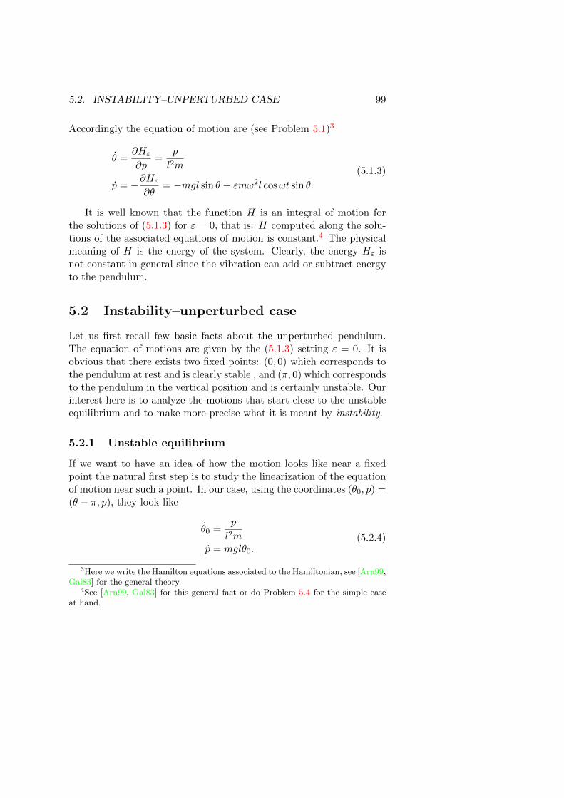
Accordingly the equation of motion are (see Problem 5.1)3

✓ =@H"

@p=

p

l2m

p = �@H"

@✓= �mgl sin ✓ � "m!2l cos!t sin ✓.

(5.1.3)

It is well known that the function H is an integral of motion forthe solutions of (5.1.3) for " = 0, that is: H computed along the solu-tions of the associated equations of motion is constant.4 The physicalmeaning of H is the energy of the system. Clearly, the energy H" isnot constant in general since the vibration can add or subtract energyto the pendulum.

5.2 Instability–unperturbed case

Let us first recall few basic facts about the unperturbed pendulum.The equation of motions are given by the (5.1.3) setting " = 0. It isobvious that there exists two fixed points: (0, 0) which corresponds tothe pendulum at rest and is clearly stable , and (⇡, 0) which correspondsto the pendulum in the vertical position and is certainly unstable. Ourinterest here is to analyze the motions that start close to the unstableequilibrium and to make more precise what it is meant by instability.

5.2.1 Unstable equilibrium

If we want to have an idea of how the motion looks like near a fixedpoint the natural first step is to study the linearization of the equationof motion near such a point. In our case, using the coordinates (✓

0

, p) =(✓ � ⇡, p), they look like

✓0

=p

l2mp = mgl✓

0

.(5.2.4)

3Here we write the Hamilton equations associated to the Hamiltonian, see [Arn99,Gal83] for the general theory.

4See [Arn99, Gal83] for this general fact or do Problem 5.4 for the simple caseat hand.


Let !p =q

gl , the general solution of (5.2.4) is

(✓0

(t), p(t)) = (↵e!p

t + �e�!p

t,ml2!p{↵e!p

t � �e�!p

t}),where ↵ and � are determined by the initial conditions. Note that if theinitial condition has the form ↵(1, ml

pgl) it will evolve as ↵e!p

t(1, mlpgl).

While if the initial condition is of the form �(1, �mlpgl) it will evolve

as �e�!p

t(1, �mlpgl). In other words the directions (1, ml

pgl) and

(1, �mlpgl) are invariant for the linear dynamics. The first direction

is expanded (and because of this is called unstable direction) while thesecond is contracted (stable direction).

��@

@@@@@@@@@@@@@

��

��✓

@@I

@@R

Figure 5.1: Unstable fixed point (phase portrait)

Let us imagine to start the motion from an initial condition of thetype (⇡ + ✓

0

, 0), ✓0

2 [��, �], where � 10�4 represents the precisionwith which we are able to set the initial condition (one tenth of amillimeter); what will happen under the linear dynamics?

Our initial condition correspond to choosing, at time zero, ↵ =� �

2

. As time goes on the coe�cient of � becomes exponentiallysmall while the coe�cient of ↵ increases exponentially, thus a goodapproximation of the position of the pendulum after some time is givenby

✓0

(t) ⇡ ↵e!p

t. (5.2.5)

Since !p ⇡ 3.13 seconds�1, it follows that after about 2.5 seconds theposition of the pendulum can be anywhere up to a distance of about10 centimeters from the unstable position.

5.2. INSTABILITY–UNPERTURBED CASE 101

This means that the unstable position is really unstable and if wetray, as best as we can, to put the pendulum in the unstable equilibrium(always imagining that the friction has been properly reduced) it willtypically fall after few seconds and it will fall in a direction that weare not able to predict (since it depend on the sign of �, our unknownmistake). Nevertheless, after the ideal pendulum starts falling in onedirection the subsequent motion is completely predictable, as we willsee shortly.

An obvious objection to the above analysis is that I did not showthat the linearized equation describes a motion really close to the oneof the original equations. The answer to this question is particularlysimple in this setting and is addressed in the next subsection.

5.2.2 The unstable trajectories (separatrices)

Given the already noted fact that, for " = 0, H is a constant of motion,the phase space M is naturally foliated in the level curves of H, onwhich the motion must take place. This allows us to obtain a fairlyaccurate picture of the motions of the unperturbed pendulum. In fact,the level curves are given by the equations

p2

2l2m�mgl cos ✓ = E

where E is the energy of the motion. It is easy to see that E = �mglcorresponds to the stable fixed point (✓, p) = (0, 0); �mgl < E <

mgl corresponds to oscillations of amplitude arccosh

Emgl

i

; E > mgl

corresponds to rotatory motions of the pendulum. The last case E =mgl is of particular interest to us: obviously it corresponds to theunstable fixed point (⇡, 0), yet there are other two solution that travelon the two curves

p = ±mlp

2lg(1 + cos ✓).

This two curves are the ones that separate the oscillatory motionsfrom the rotatory ones and, for this reasons, are called separatrices.It is very important to understand the motion along such trajectories,luckily the two di↵erential equations

✓ = ±r

2g

l(1 + cos ✓). (5.2.6)


⇢⇡�⇠

�⇡ ⇡

Figure 5.2: Unperturbed pendulum (phase portrait)

can be integrated explicitly (see Problem 5.5) yielding, for ✓(0) = 0,

✓(t) = 4 arctan e±!p

t � ⇡. (5.2.7)

This orbits are asymptotic to the unstable fixed point both at t !+1 and at �1 and, for |t| large, agree with the linear behaviour ofsection 5.2.1. This situation is somewhat atypical as we will see briefly.

5.3 The perturbed case

5.3.1 Reduction to a map

The motion of the above system takes place on the cylinder M =S1 ⇥ R. By the theorem of existence and uniqueness for the solutionsof di↵erential equations follows immediately the possibility to define themaps �t

" : M ! M associating to the point (✓, p) the point reachedby the solution of (5.1.3) at time t, when starting at time 0 from theinitial condition (✓, p). In such a way we define the flow �t

" associatedto the (5.1.3).

Clearly �0

"(✓, p) = (✓, p), that is the map corresponding at time zerois the identity. Moreover, if " = 0 the system is autonomous (the vectorfield does not depend on the time) hence the flow defines a group: foreach t, s 2 R

�t+s0

(✓, p) = �t0

(�s0

(✓, p)).

5.3. THE PERTURBED CASE 103

This corresponds to the obvious fact that the motion for a time t + scan be obtained first as the motion from time 0 to time s, and thenpretending that the time s is the initial time and following the motionfor time t.

Of course, the above fact does not hold anymore when " 6= 0. Inthis case, the maps �t

" depend from our choice of the initial time (if wedefine them by starting from time 1 instead then time 0, in general weobtain di↵erent maps). Nevertheless, due to the fact that the externalforce is periodic something can be saved of the above nice property.

Let us define the map T" : M ! M by

T" = �2⇡!

" ,

then (see Problem 5.3), for each n 2 Z,

Tn" = �

2n⇡

!

" . (5.3.8)

The interest of (5.3.8) is that, for many purposes, we can study themap T" instead than the more complex object �t

". Morally, it meansthat if we look at the system stroboscopically, that is only at the times2⇡! n with n 2 Z, then it behaves like an autonomous (time independent)system.5 Another interesting fact is that the flow �t

" (and hence alsothe map T") is area preserving (see Problem 5.7).6

5.3.2 Perturbed pendulum, " 6= 0

The situation for the case " 6= 0 is more complex and no easy way existsto study these motions.

As a general strategy, to study the behavior of a system (in ourcase the map T") it is a good idea to start by investigating simple casesand then move on from there. In our systems the simplest motionconsists of the equilibrium solutions. These are the time independentsolutions.7 Because of the special type of perturbation chosen the fixed

5This is a very simple case of a very fruitful an general strategy: to look at thesystem only when some special event happens–in our case at each time in which thesuspension point has its maximum height. See 6.2 if you want to know more.

6This also is a special instance of a more general fact: the Hamiltonian natureof the system, see [Arn99, Gal83] if you want to know more.

7That is, equilibrium solutions for the map T"

. These are periodic solutions for

the flows of period 2⇡!

. In fact, T"

x = x means �2⇡! x = x.


points of the system for the case " = 0 remain unchanged when " 6= 0(see Problem 5.8 for a brief discussion of a more general case).

Next, we can study the infinitesimal nature of the fixed points. Itis natural to expect that the nature of the two fixed points does notchange if " is small, yet to verify this requires some checking. We willdiscuss explicitly only the fixed point (⇡, 0).

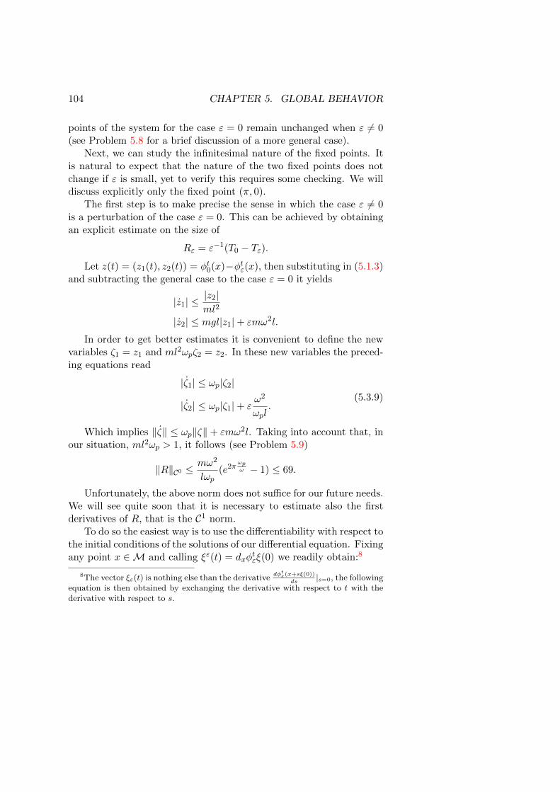
The first step is to make precise the sense in which the case " 6= 0is a perturbation of the case " = 0. This can be achieved by obtainingan explicit estimate on the size of

R" = "�1(T0

� T").

Let z(t) = (z1

(t), z2

(t)) = �t0

(x)��t"(x), then substituting in (5.1.3)

and subtracting the general case to the case " = 0 it yields

|z1

| |z2

|ml2

|z2

| mgl|z1

|+ "m!2l.

In order to get better estimates it is convenient to define the newvariables ⇣

1

= z1

and ml2!p⇣2 = z2

. In these new variables the preced-ing equations read

|⇣1

| !p|⇣2|

|⇣2

| !p|⇣1|+ "!2

!pl.

(5.3.9)

Which implies k⇣k !pk⇣k+ "m!2l. Taking into account that, inour situation, ml2!p > 1, it follows (see Problem 5.9)

kRkC0 m!2

l!p(e2⇡

!

p

! � 1) 69.

Unfortunately, the above norm does not su�ce for our future needs.We will see quite soon that it is necessary to estimate also the firstderivatives of R, that is the C1 norm.

To do so the easiest way is to use the di↵erentiability with respect tothe initial conditions of the solutions of our di↵erential equation. Fixingany point x 2 M and calling ⇠"(t) = dx�t

"⇠(0) we readily obtain:8

8The vector ⇠"

(t) is nothing else than the derivatived�

t

"

(x+s⇠(0))ds

|s=0, the following

equation is then obtained by exchanging the derivative with respect to t with thederivative with respect to s.

5.4. INFINITESIMAL BEHAVIOR (LINEARIZATION) 105

⇠"1

=⇠"2

l2m⇠"2

= �mgl cos ✓ ⇠"1

� "m!2l cos!t cos ✓ ⇠"1

(5.3.10)

One can then estimate the C1 norm of R by estimating k⇠"(2⇡! ) �⇠0(2⇡! )k, since ⇠"(2⇡! ) = D

(✓,p)T"⇠"(0). Doing so one obtains9

kRkC1 2m!2

l!pe3⇡

!

p

! := d1

690. (5.3.11)

5.4 Infinitesimal behavior (linearization)

As a first application of the above considerations let us study the lin-earization of T" at xf = (⇡, 0). From (5.3.10) follows (see Problem5.12)

Dxf

T0

=

cosh 2⇡!p

!

sinh

2⇡!

p

!

ml2!p

ml2!p sinh2⇡!

p

! cosh 2⇡!p

!

!

Dxf

T" = Dxf

T0

+O(d1

") (5.4.12)

The eigenvalues of Dxf

T" are then �" = e2⇡!

p

! + O(d2

"),10 ��1

" ,where d

2

= 2d1

!pml2 ' 4400. In addition, calling v", hv", v0i = 1,the eigenvector associate to �", holds true kv

0

� v"k d3

", d3

=4��1

0

!2

p!2l4d

1

' 1200.11

Clearly, if " is su�ciently small, then �" > 1. This means that thehyperbolic nature of the unstable fixed point remains unchanged under

9The following bounds are not sharp, working more one can obtain better esti-mates but this would not make much of a di↵erence in the sequel.

10In this chapter we will adopt the strict convention that O(x) means a quantitybounded, in absolute value, by x.

11This follows by the fact that the eigenvalues of Dx

f

T0 are e±2⇡!

p

! ' (23)±1, asimple perturbation theory of matrices (see Problems 5.10, 5.11) and the alreadymentioned fact that the map T

"

is area preserving, thus the determinant of itsderivative must be one.


small perturbations (see Problem 5.13 for a case when the perturbationis not so small).12

If one does a similar analysis at the fixed point (0, 0) one finds thatthe eigenvalues have modulus one: that is the infinitesimal motion is arotation around the fixed point, exactly as in the " = 0 case.

Hence the comments made at the end of subsection 5.2.1 for theunperturbed pendulum hold for the perturbed pendulum as well. Onlynow the is no longer an integral of motion (the energy) that controlsglobally the behavior of the system.

Imagining that the map is linear (which is clearly false but, as wewill see, qualitatively not so wrong) this would mean that the distancebetween two trajectories can be expanded by almost a factor 23 in asecond. Initial conditions that are � close at time zero will be about23� far apart after 1 second. If such a state of a↵air could persist(and we will see it may) after one minute the two configurations woulddi↵er roughly by a factor 1080�, which means that not even knowingthe initial condition plus or minus a quark could we predict the finalone. This is certainly a rather worrisome perspective but much morework it is needed to decide if this may be indeed the case.

5.5 Local behavior (Hadamard-Perron Theo-rem)

The next step is to try to go from the above infinitesimal analysis to alocal picture in a small neighborhood of the fixed points.

It is natural to expects that the two fixed points are still stable andunstable respectively, yet this is a far from trivial fact.

The stability of the point (0, 0) can be proven by invoking the socalled KAM Theorem (this exceeds the scope of the present book andwe will not discuss such matters, see [Gal83] for such a discussion).13

12As we will see later in detail, hyperbolicity means that there is a direction inwhich the maps expands (the eigenvector vu

"

associated to the eigenvalue �"

) and adirection in which the map contracts (the eigenvector vs

"

associated to the eigenvalue��1"

)13In some sense this implies that we can indeed predict the motion for an extremely

long time if we consider only oscillations close to the configuration (0, 0), so in thatcase the assumption that the pendulum is isolated is legitimate. Yet, this dependson the precision we are interested in and tends to degenerate if the amplitude of

5.5. LOCAL BEHAVIOR (HADAMARD-PERRON THEOREM)107

The study of the local behavior around the point xf is insteada bit easier and can be performed by applying the Hadamard-PerronTheorem 2.4.2 to conclude that, in a neighborhood of (⇡, 0), there existstwo curves xu" (s) = (✓u" (s), p

u" (s)), x

s"(s) that are invariant with respect

to the map T". Namely, there exists �" > 0 such that T"xs"([��", �"]) ⇢xs"([��", �"]) and T�1

" xu" ([��", �"]) ⇢ xu" ([��", �"]); this are called thelocal stable and unstable manifold of zero, respectively. Essentially�" is determined by the requirement that the non-linear part of T" besmaller than the linear part.

Clearly, for " = 0 xs0

= xu0

= x0

and it coincides with the homoclinicorbit of the unperturbed pendulum. In addition, by Hadarmd-Perronand the estimates of the previous section, we can choose �" such that

kxu" � x0

k 2d3

"kx0

k. (5.5.13)

and the analogous for the stable manifold. We have so obtained a localpicture of the behavior of the map T", yet this does not su�ce to answerto our original question. To do so we need to follow the motion for atleast a full oscillation: this requires really a global information.

To gain a more global knowledge we can try to construct largerinvariant set for the map T". A natural way to do so is to iterate: defineW u = [1

n=0

Tn" x

u([��", �"]). Since T"xu([��", �"]) � xu([��", �"]), it isclear that each time we iterate we get a longer and longer curve. Theset W u is then clearly a manifold and it is called the global unstablemanifold.14

The global manifold, as the name clearly states, it is a global object:it carries information on the dynamics for arbitrarily long times. Yet,the procedure by which it has been defined is far from constructiveand the truth is that, besides the sketchy considerations above, at themoment we know very little of it. The next step is to gain some moredetailed understanding of a large portion of W u.

the oscillations is rather large. A complete analysis would be a very complicatedmatter but we will have an idea of the type of problems that can arise by consideringextremely large oscillations, close to a full rotation of the pendulum.

14Applying the above procedure to the unperturbed problem yields the full sepa-ratrix.


5.6 A more global understanding (the Melnikovmethod)

From the above considerations follows that the stable and unstablemanifolds (✓s"(s), p

s"(s)), (✓

u" (s), p

u" (s)), |s| �", of T" at 0, are " close

to the homoclinic orbit of the unperturbed pendulum, (✓0

(t), p0

(t)),✓0

(0) = 0.Note, however, that while x

0

= (✓0

, p0

) is invariant under the un-perturbed flow, the same does not apply to (✓s,u" (s), ps,u" (s)) under �t

".Indeed the invariant object is the time-space surface (⌧, xs,u" (s, ⌧)) :=(⌧,�⌧

" (✓s"(s), p

s"(s))) where (s, ⌧) 2 [��", �"] ⇥ [0, 2⇡! ] and and ⌧ = t

mod 2⇡! .15

Clearly, we can choose freely the parameterization of our curves insuch a surface and some are more convenient than others. The separa-trix of the unperturbed pendulum is most conveniently parametrizedby time, hence �t(✓

0

(s), p0

(s)) = (✓0

(s + t), p0

(s + t)). We wish toparameterize the perturbed manifold in a convenient way, one simplepossibility could be to impose ✓u" (�s) = ✓

0

(�s), ✓s"(s) = ✓0

(s), yetthis happens to be not very helpful for our goals. To find a more con-venient parameterization it is necessary to do first some preliminaryconsiderations.

To grow the above manifolds, as explained in the previous section,we can start from some remote time �Sn := 2⇡!�1n, n 2 N, (Sn for thestable) and then iterate forward the unstable manifold and backwardthe stable. This is better done by using the flow and the equationsof motion. To this end, it turns out to be specially smart to first useglobal coordinates similar to the ones used to simplify equation (5.3.9)and then to consider local coordinates adapted to the separatrix of theunperturbed pendulum. Namely, let us introduce p =: ml2!pp, ✓ =: ✓.Note that such a change of coordinate is not symplectic, hence we haveto compute the resulting Hamiltonian in the new coordinates. It is

15A standard way to bring the present non-autonomous setting in the more famil-iar autonomous one is to introduce the fake variables (', ⌘) 2 S1 ⇥ R and the new,time independent, Hamiltonian H

"

(✓, p,', ⌘) := H"

(✓, p,') + 2⇡!

⌘. The Hamiltonequations yield '(t) = 2⇡

!

t+'(0) and hence the equations for ✓, p reduce to (5.1.3).Since H

"

is now conserved under the motion we can restrict the system to the threedimensional manifold H

"

= 0. In such a manifold we have the weak stable andunstable manifolds (now flow invariant) (xs,u

"

(s,'),',� 2⇡!

H"

((xs,u

"

(s,'),')).

5.6. MELNIKOV METHOD 109

easy to verify that the Hamiltonian becomes

H" :=!p

2p2 � !p cos ✓ � "

!2

l!pcos!t cos ✓ =: H

0

+ "H1

(5.6.14)

which yields the corrects equations of motion.

˙✓ = !pp

˙p = �!p sin ✓ � "!2

l!pcos!t sin ✓

(5.6.15)

We will use the vector notation x := (✓, p).16 In such coordinates weconsider the stable and unstable manifolds xs"(s), x

u" (s) for the per-

turbed pendulum and the separatrix x0

(s) for the unperturbed pendu-lum and we define

xs,u" (s, t) = �t"x

s,u" (s). (5.6.16)

If we call �t" the flow started at the time �Sn (Sn, respectively),17 and

we consider t = Sm (t = �Sm), m < n, we obtain new curves that aremuch longer than the original ones and still describe the unstable andstable manifolds (albeit with a di↵erent parameterization). Next, wedefine the vectors

⌘1

(s) :=x0

(s)

kx0

(s)k =Jrx0(s)H0

krx0(s)H0

k and ⌘2

(s) :=rx0(s)H0

krx0(s)H0

k .

This form an orthonormal basis of R2 (see Problem 5.14). We canthen consider the map F (a, b) := x

0

(a) + b⌘2

(a). One can check thatdetDF

(a,0) 6= 0, hence F defines a change of coordinates in a neigh-borhood of x

0

. Note that in the new coordinates the unperturbedseparatrix x

0

reads {(a, 0)}.In analogy with a standard approach to the Hadamard-Perron The-

orem (see 2.4.2) it seems natural to have our curves parametrized so

16Using such a notation equations (5.6.15) take the more compact form

x = Jrx

H"

; J =

✓0 1�1 0

◆.

17Remember that the flow started at such times is exactly the same than the flowstarted at time zero, see subsection 5.3.1.


that, in the new coordinates, they have the same first component. Thismeans that we would like to have hxu" (s)�x

0

(s), ⌘1

(s)i = 0. We can ob-viously arrange such a property for the original curve at the tine �Sn,but can we keep it thruought the growth process? A simple possibilityis to flow di↵erent points for di↵erent times as to maintain the wantedproperty. That is to look for a ⌧ such that,18

G(s, t, ⌧) := hxu" (s, t+ ⌧)� x0

(s+ t), ⌘1

(s+ t)i = 0. (5.6.17)

Since, by construction, G(s, 0, 0) = 0 we can apply the implicit functiontheorem, to prove the existence of the wanted function ⌧(s, t). Thenecessary condition to do so is a lower bound on |@⌧G|. Next, settingxu" (s, t+ ⌧) =: x

0

(s+ t) + "xu1

(s, t, ⌧),

@⌧G(s, t, ⌧) = hJrxu

"

(s,t+⌧)H", ⌘1(s+ t)i= krxu

0 (s+t)H0

k+ "O(kD2H"k kxu1

k+ krxu

0H

1

k).(5.6.18)

By (5.5.13) we have kxu" (s)�x0

(s)k kx0

(s)k�1 2d3

", for s �Tn0 . In

addition, from (5.2.7) and Problem 5.6 follows sin ✓0

(t) = 2 sinh!p

t(cosh!

p

t)2'

2e!p

t, for t ⌧ 0. Moreover p0

=q

2(1 + cos ✓0

) = 2(cosh!pt)�1. Then

krx0(t)H0

k � !pp2

e�!p

|t|.Accordingly, remembering equations(5.5.13) and (5.6.18) we can

apply the Implicit Function Theorem provided kxu1

(s, t, ⌧)k 4d3

e�!p

|s+t|

and " (8d3

)�1 ' 10�4. Hence the wanted function ⌧(s, t) is well de-fined and19

@⌧

@t= � @tG

@⌧G= O(64d

3

"). (5.6.19)

It is then convenient to define

�u(s, t) = "�1hxu" (s, t, ⌧)� x0

(s, t), rx0(s+t)H0

i = kxu1

k krx0H0

k.

Using (5.1.3) we can di↵erentiate �u with respect to t and since

18Note that, in so doing, we will construct an object di↵erent from the startingone associated to a fixed Poincare section.

19Indeed, @t

G = hJrx

u

"

H"

�Jrx0H0, ⌘1i+ "hxu

1 , ⌘1i = "O(3!p

kxu

1k+ krx0H1k).

5.6. MELNIKOV METHOD 111

Jrxu

"

H" = Jrx0H" + "JD2

x0H"xu

1

+O( "2

2

kD3H0

k |xu1

|2), we have

d�u

dt(s, t) = "�1hJrxu

"

H"(1 + ⌧),rx0Hi+ hxu1

, D2

x0H

0

Jrx0H0

i

=n

hJrx0H1

, Jrx0H0

i+O(2"!pd3e!p

(t+s)|�u1

|)o

(1 + |⌧ |1)

+O(|⌧ |1|�u1

|!p).

(5.6.20)

We can thus integrate the Gronwald type inequality (5.6.20), (if indoubt, see Problem 5.9), and, assuming 256!pd3" < 1 (roughly " 10�5),

|�u(s, t)| 8!2

l!pe2!p

(t+s).

Hence, kxu1

k 24!2e!p

(t+s)

l!2p

< 4d3

e�!p

|t+s|, provided it holds true t+s (2!p)�1 ln

h

d3l!2p

6!2

i

=: t0

' 0.6.

To gain complete control on the stable manifold we need only todiscuss the issue of the time shift. On the one hand, all is needed is tochange t+ ⌧(s, t) to zero ( mod 2⇡

! ). On the other hand if ⇢ 2 [0, 2⇡! ],then ⇣(⇢) := �⇢

"(x)��⇢0

(y) can be estimated, slightly refining (5.3.9), by

integrating k⇣k (!p + " !2

!p

l )k⇣k+ " !2

!p

l |✓0(t+ s+ ⇢)|. This shows thatwe can extend the unstable manifold till a neighborhood of x

0

(�S2

)and still keep the an inequality of the type kxu" � x

0

k 3d3

kx0

k.Finally, substituting the above estimate in (5.6.20), yields

d�u

dt(s, t) = hJrx0H1

, Jrx0H0

i+O⇣

544 · l�1!2d3

"e2!p

(t+s)⌘

.

Integrating from 0 to Sm, m 2 N for s+ Sm t0

, yields

�u(s, Sm) =

Z Sm

0

{H1

(·, t1

), H}x0(s+t1)dt1 +�u(s, 0) +O

⇣

"d4

e2!p

(s+Sm

)

⌘

=

Z

0

�Sm

{H1

(·, t1

), H}x0(s+Sn

+t1)dt1 +�u(s, 0) +O

⇣

"d4

e2!p

(s+Sm

)

⌘

(5.6.21)

where d4

:= 272 · !2

!p

ld3 ' 4 · 106 and the curly brackets stand for the

so called Poisson brackets ({f, g}x = hJrxf, rxgi).


The stable manifold can be studied similarly, yet it is faster to de-fine the transformation (✓, p) = (�✓, p), and note that ��t

" ( (x)) = (�t

"(x)). Accordingly, xs"(s,�t) = (xu" (�s, t)). Also, one easilychecks that, calling ⌧ s(s, t) the time shift arising from the analogous of(5.6.17), ⌧ s(s,�t) = ⌧(�s, t). In addition, |⌧(s, Sm)| 65d

3

"Sm.Setting �(�) := �u(�s� Sm, Sm) ��s(s+ Sm,�Sm), for all � 2

[�t0

, t0

], we finally have

kxu" (�� Sm, Sm)� xs"(Sm � �, Sm)k 644⇡! � p

!d3

"Sm +�(�)

�(�) =

Z 1

�1{H

1

, H}x0(t+�)dt+O⇣

"2d4

e2!p

|�|⌘

,

(5.6.22)

provided m > 2. The integral in (5.6.22) is called Melnikov integral andprovides an expression, at first order in ", of the distance between thestable and the unstable manifold. All we are left with is to computethe integrals in (5.6.22). This turns out to be an exercise in complexanalysis and it is left to the reader (see Problem 5.15), the result is:20

Z 1

�1{H

1

(·, t), H}x0(t+�)dt = 8⇡ml!4e

� ⇡!

2!p

!2

p(e⇡!

!

p � 1)sin!�.

We have thus gained a very sharp control on the shape of the abovemanifolds.21 In particular, �(±1/4) ' ±76 +O(4 · 107") 6= 0 provided

20A simple computation yields:

{H1, H}x0(t+s) = �!2

lp(t+ s) cos!t sin ✓(t+ s).

Then, by using (5.2.7) and looking at Problem 5.6, one readily obtains:

{H1, H}x0(t) = 4

!2

l

cos!(t� s) sinh!p

t

(cosh!p

t)3.

Finally, use Problem 5.15.21Note that " must be exponentially small with respect to !. In many concrete

problems (notably the so called Arnold di↵usion [?]) it happens that this it is notthe case. One can try to solve such an obstacle by computing the next terms of the" expansion of �. In fact, it turns out that it is possible to express � as a powerseries in " with all the terms exponentially small in ! [?]. Yet this is a quite complextask far beyond our scopes.

5.7. GLOBAL BEHAVIOR (AN HORSESHOE) 113

" 1.5 · 10�6, that is the two manifolds intersect. To understand a bitbetter such an intersection (we would like to know that in the region� 2 [�1/4, 1/4] there is only one transversal intersection) its su�ces tonotice that (5.6.20) provides a control on the angle between xu" and x

0

.This intersections are called homoclinic intersection and their very

existence is responsible for extremely interesting phenomena as can bereadily seen by trying to draw the stable and unstable manifolds (seeFigure 5.3 for an approximate first idea); we will discuss this issue indetail shortly.22

⇢⇡�⇠

�⇡ ⇡

Figure 5.3: Perturbed pendulum

We have gained much more global information on the map T", yet itdoes not su�ce to answer to our question. The next section is devotedto obtaining a really global picture. Up to now we have used mainlyanalytic tools. Next, geometry will play a much more significant role.23

5.7 Global behavior (an horseshoe)

We want to explicitly construct trajectories with special properties. Astandard way to do so is to start by studying the evolution of appro-priate regions and to use judiciously the knowledge so gained. Let us

22Note that the intersection corresponds to an homoclinic orbit for the map T"

(that is, an orbit which approaches the fixed point xf

both in the future and in thepast). This is what it is left of the homoclinic orbit of the unperturbed pendulum.

23What comes next is the first example in this book of what is loosely called a

dynamical argument.


see what this does mean in practice.The starting point is to note that we understand the shape of the

invariant manifold but not very well the dynamics on them, this is ournext task. Since points on the unstable manifolds are pulled apart bythe dynamics, the estimate must be done with a bit of care. In fact, wewill use a way of arguing which it typical when instabilities are present,we will see many other instances of this type of strategy in the sequel.

For each x in the unstable manifold (zero included) let us callDu

xT" := DxT"vu(x), where vu(0) = vu and if x = xu" (t) then vu(x) =kxu" (t)k�1xu" (t), that is the derivative of the map computed along theunstable manifold. A useful idea in the following is the concept of fun-damental domain. Define ↵ : R

+

! R+

by xu" (t) = xu" (↵(t)). Then[t,↵(t)] is a fundamental domain and has the property that, settingti := ↵i(t), the sets ↵i[t

0

, t1

] intersect only at the boundary.

Lemma 5.7.1 (Distortion) For each x, y in the same fundamentaldomain of the unstable manifold, �

0

> 0, and n 2 N such that kTn" xk

�0

, holds24

e��0C2 �

�

�

�

DuxT

n"

DuyT

n"

�

�

�

�

e�0C2 ,

where C2

= supt0

�

�

�

↵(t)↵(t)

�

�

�

.

Proof. The proof is a direct application of the chain rule:

�

�

�

�

DuxT

n"

DuyT

n"

�

�

�

�

=nY

i=1

�

�

�

�

�

DuT ix

T"

DuT iy

T"

�

�

�

�

�

Exp

"

nX

i=1

| log(|DuT ixT")� log(|Du

T iyT"|)|#

Exp

"

nX

i=1

C2

kT ix� T iyk#

= Exp

"

nX

i=1

C2

kxu" (ti)� xu" (ti�1

)k#

eC2�0 .

The other inequality is obtained by exchanging the role of x and y. ⇤

Next we would like to consider the evolution of a small box con-structed around the fix point.

24This quantity is commonly called Distortion because it measures how much themap di↵ers from a linear one (notice that if T is linear then D

x

T

D

y

T

= 1). Although

apparently an innocent quantity, it is hard to overstate its importance in the studyof hyperbolic dynamics.

5.7. GLOBAL BEHAVIOR (AN HORSESHOE) 115

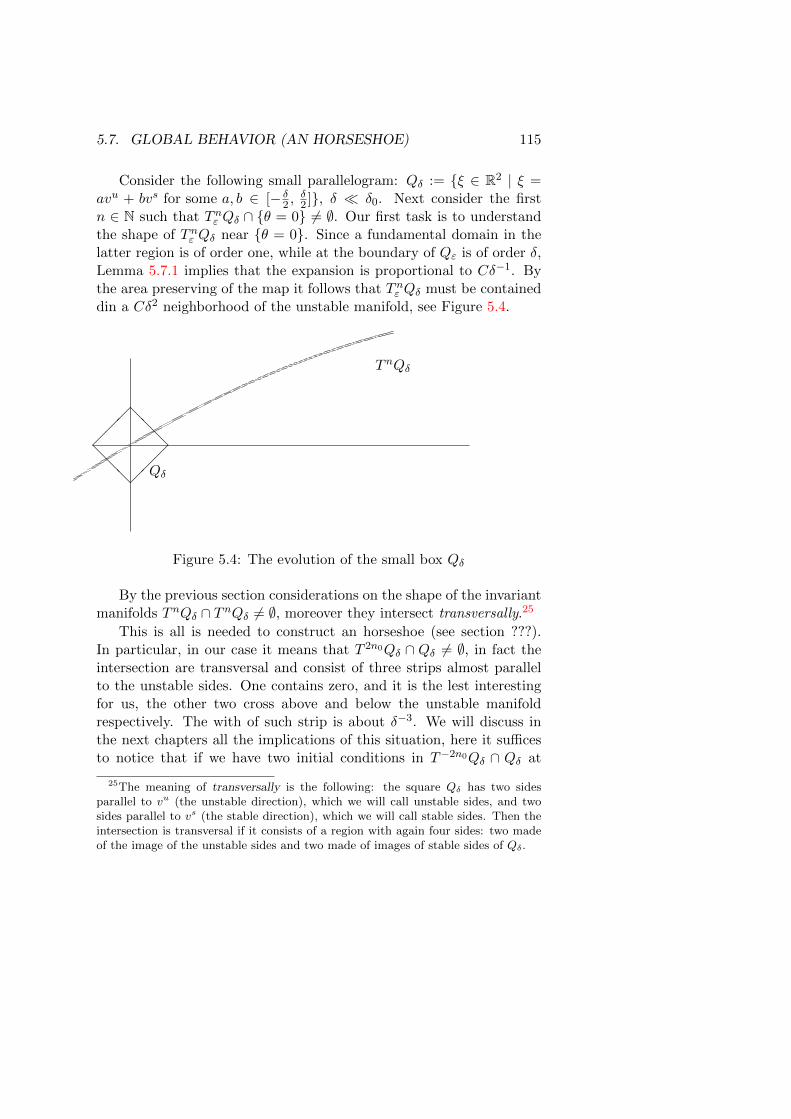
Consider the following small parallelogram: Q� := {⇠ 2 R2 | ⇠ =avu + bvs for some a, b 2 [� �

2

, �2

]}, � ⌧ �0

. Next consider the firstn 2 N such that Tn

" Q� \ {✓ = 0} 6= ;. Our first task is to understandthe shape of Tn

" Q� near {✓ = 0}. Since a fundamental domain in thelatter region is of order one, while at the boundary of Q" is of order �,Lemma 5.7.1 implies that the expansion is proportional to C��1. Bythe area preserving of the map it follows that Tn

" Q� must be containeddin a C�2 neighborhood of the unstable manifold, see Figure 5.4.

@@@

��

��

@@@ Q�

TnQ�

Figure 5.4: The evolution of the small box Q�

By the previous section considerations on the shape of the invariantmanifolds TnQ� \ TnQ� 6= ;, moreover they intersect transversally.25

This is all is needed to construct an horseshoe (see section ???).In particular, in our case it means that T 2n0Q� \ Q� 6= ;, in fact theintersection are transversal and consist of three strips almost parallelto the unstable sides. One contains zero, and it is the lest interestingfor us, the other two cross above and below the unstable manifoldrespectively. The with of such strip is about ��3. We will discuss inthe next chapters all the implications of this situation, here it su�cesto notice that if we have two initial conditions in T�2n0Q� \ Q� at

25The meaning of transversally is the following: the square Q�

has two sidesparallel to vu (the unstable direction), which we will call unstable sides, and twosides parallel to vs (the stable direction), which we will call stable sides. Then theintersection is transversal if it consists of a region with again four sides: two madeof the image of the unstable sides and two made of images of stable sides of Q

�

.


@@@

@@@

��

��

��

@@@@@@�

��

��

��

��

��

��

Figure 5.5: Horseshoe construction

a distance h, after 2n0

iterations the two points will be in Q� againbut at a distance h"�1. Since to decide if after that there will bea rotation or an oscillation we need to know the final position witha precision of order �, we need to know the initial position with aprecision O(�") = O(�3).

Note that in the above construction we have lost almost all thepoints, only the ones that come back to Q� at time 2n

0

are under con-trol. Nevertheless, we can consider the set ⇤ := [k2Z

T

T 2kn0" Q�. This

is clearly a measure zero set, yet it is far from empty (it contains un-countably many points) and it is made of points that at times multipleof 2n

0

are always in Q�. When they arrive in Q� they will rotate if theyare above the separatrices and oscillate otherwise. Let us call this twosubset of Q� R and O. Given a point ⇠ 2 Q� we can associate to it thedoubly infinite sequence � 2 {0, 1}Z by the rule �i = 1 i↵ T 2n0i⇠ 2 R.The reader can check that the correspondence is onto.

5.8 Conclusion–an answer

If " = 10�6 and � is a millimeter then we need to know the initialcondition with a precision of 10�9 meters if we want to decide if thepoint will come back or rotate when it will get almost vertical again(this will happen in about 6 seconds). By the same token if we want toanswer the same question, but for the second time the pendulum getclose to the unstable position, we need to know the initial condition

PROBLEMS 117

with a precision of the order 10�15 meters, and this just to predict themotion for about 12 seconds.26

We can finally answer to our original question:

Answer: NO!

Nevertheless, as we mentioned at the beginning, the above answerit is not the end of the story. In fact, there exists many other veryrelevant questions that can be answered.27 The rest of the book dealswith a particular type of question: can we meaningfully talk about thestatistical behavior of a system?

Problems

5.1. Derive the Lagrangian, Hamiltonian and equations of motionsfor a pendulum attached to a point vibrating with frequency !and amplitude ". (Hint: see [LL76, Gal83] on how to do suchthings. Remember that two Lagrangian that di↵er by a totaltime derivative give rise to the same equation of motions and arethus equivalent.)

5.2. Consider the systems of di↵erential equations x = f(x), x 2 Rn

and f smooth and bounded. Prove that the associated flow form agroup. (Hint: use the uniqueness of the solutions of the ordinarydi↵erential equation)

5.3. Consider the systems of di↵erential equations x = f(x, t), x 2 Rn

and f smooth, bounded and periodic in t of period ⌧ . Let �t bethe associated flow. Define T = �⌧ , prove that Tn = �n⌧ .

26Remark that it is not just a matter of precision on the initial condition, it isalso a matter of how one actually does the prediction. If the method is to integratenumerically the equation of motion, then one has to insure that the precision ofthe algorithm is of the order of 10�15. This maybe achieved by working in doubleprecision but if one wants to make predictions of the order of one minute it is quiteclear that the numerical problem becomes very quickly intractable.

27For example: which type of motions are possible? This is a qualitative question.Such type of questions give rise to the qualitative theory of Dynamical Systems[PT93, HK95], an extremely important part of the theory of dynamical systems,although not the focus here.


5.4. Show that the Hamiltonian is a constant of motion for the pen-dulum. (Hint: Compute the time derivative)

5.5. Prove (5.2.7). (Hint: Write (5.2.6) in the integral form

t =

Z t

0

✓(s)q

2gl (1 + cos ✓(s))

ds.

Using some trigonometry and changing variable obtain

t =

Z ✓(t)

0

1

2!p cos✓2

d✓.

and compute it.)

5.6. If ✓(t) is the motion obtained in the previous problem, show that

sin ✓(t) = 2sinh!pt

(cosh!pt)2; cos ✓(t) =

2

(cosh!pt)2� 1;

cos2✓(t) + ⇡

4=

1

1 + e2!p

t.

5.7. Consider the systems of di↵erential equations x = f(x, t), x 2 Rn

and f smooth. Suppose further that divf = 0 (that isPn

i=1

@fi

@xi

=0). Show that the associated flow preserves the volume. (Hint:note that this is equivalent to saying that | det d�t| = 1, moreoverby the group property and the chain rule for di↵erentiating itsu�ces to check the property for small t. See that d�t = 1+Dft+O(t2) = eDft+O(t2). Finally, remember the formula det eA =eTrA.)

5.8. Let T, T1

: R2 ! R2 be a smooth maps such that T0 = 0 anddet(1 � D

0

T ) 6= 0. Consider the map T" = T + "T1

and showthat, for " small enough, there exists points x" 2 R2 such thatT"x" = x". (Hint: Consider the function F (x, ") = x � T"x andapply the Implicit Function Theorem to F = 0.)

5.9. Let x(t) 2 Rn be a smooth curve satisfying kx(t)k a(t)kx(t)k+b(t), x(0) = x

0

, a, b 2 C0(R,R+

), prove that

kx(t)� x0

k Z t

0

eRt

s

a(⌧)d⌧ [a(s)kx0

k+ b(s)] ds.

PROBLEMS 119

(Hint: Note that kx(t)� x0

k R t0

kx(s)kds. Transform then thedi↵erential inequality into an integral inequality. Show that ifz(t) 0 and z(t) R t

0

z(s)ds, then z(t) 0 for each t. Use thelast fact to compare a function satisfying the obtained integralinequality with the solution of the associated integral equation.)

5.10. Given two by two matrices A,B such that A has eigenvalues� 6= µ, show that the matrix A" = A+"B, for " small enough, haseigenvalues �", µ" analytic as functions of ". Show that the sameholds for the eigenvectors. (Hint:28 consider z in the resolventof A, that is (z � A)�1 exists. Then (z � A") = (z � A)(1 �"(z � A)�1B). Accordingly, if " is small enough, (z � A")�1 =�

P1n=0

"n⇥

(z �A)�1B⇤n

(z � A)�1. Finally, if �, �0 are curveson the complex plane containing � and µ, respectively, verify that

⇧" :=1

2⇡i

Z

�(z �A")

�1dz ⇧0" :=

1

2⇡i

Z

�0(z �A")

�1dz

are commuting projectors and A" = �"⇧" + µ"⇧0". Finally verify

that

�"⇧" :=1

2⇡i

Z

�z(z �A")

�1dz µ"⇧0" :=

1

2⇡i

Z

�0z(z �A")

�1dz.

The statement follows then from the fact that the right hand sideof the above equalities is written as a power series in ".29)

5.11. Given two by two matrices A,B such that A has eigenvalues� 6= µ, show that the matrix A" = A+ "B has eigenvalues �", µ"

such that |�" � �| C"kBk and |µ" � µ| C"kBk . ComputeC. (Hint: By Problem 5.10 we know that �", µ" are di↵erentiablefunction of " and the same holds for the corresponding eigenvectorv", v". Let us discuss �" since the other eigenvalues can be treatedin the same way. One possibility is to use the above formula for�"⇧" to obtain the wanted estimates.

28Of course for matrices one could argue more directly by looking at the char-acteristic polynomial. Yet the strategy below has the advantage to work even ininfinitely many dimensions (that is, for operators over Banach spaces).

29This is a very simple case of the very general problem of perturbation of pointspectrum, see [Kat66] if you want to know more.


In alternative, let v, w, hw, vi = 1 and kvk = 1, be the eigen-vectors of A, with eigenvalue � and of A⇤, with eigenvalue �,respectively. Hence ⇧

0

= v ⌦ w and k⇧0

k = kwk. Normalizev" such that hv", wi = 1. Di↵erentiate then the above constraintand the defining equation (A+"B)v" = �"v" obtaining (the primerefers to the derivative with respect to ")

Av0" +Bv" + "Bv0" = �0"v" + �"v

0"

hv0", wi = 0.

Multiplying the first for w yields �0" = hw,Bv"i+ "hw,Bv0"i. Set-

ting A := A� �⇧0

we have

v0" = (�� A)�1

⇥

Bv" + "Bv0" � �0"v" � (�� ")v

0"

⇤

.

Next, consider "0

such that, for " < "0

holds

kv0"k 4k(�� A)�1k kBk kwk = 4k(�� A)�1k kBk k⇧0

k =: C0

,(5.8.23)

then kv"�vk "C0

and |�0"| kBk kwk(1+2"C

0

). If 4"0

C0

< 1,then, indeed, (5.8.23) holds true. )

5.12. Compute D0

T . (Hint: solve (5.3.10) for " = 0, ✓ = ⇡, p = 0 andt = 2⇡

! .)

5.13. Compute D0

T" and see that, if ! is su�ciently large, the eigen-values have modulus one (the unstable point becomes stable!).

(Hint: setting ⇠ := ⇠1

equation (5.3.10) yields ⇠ = !2

p⇠+"!2

l cos!t⇠.

It is then convenient to write ⇠ := ⇠+"⌘+"2⇣ where ¨⇠ = !2

p ⇠ and

⌘ = !2

p⌘ + !2

l cos!t ⇠. One can look for a solution of the latterequation of the form

⌘ = Ae!p

t cos!t+Be!p

t sin!t+ Ce�!p

t cos!t+De�!p

t sin!t.

This allows to compute D0

T"(↵,�) = (⇠1

(2⇡! ), ⇠2

(2⇡! )) + O("2),where (⇠

1

(0), ⇠2

(0)) = (↵,�). Finally one can verify that, for "small and ! large enough the eigenvalues of D

0

T" are imaginary,hence the equilibrium is linearly stable. )

5.14. Given an Hamiltonian H : R2 ! R, for each solution x(t) of theassociated equations of motion show that hrx(t)H, x(t)i = 0.

NOTES 121

5.15. Compute the following integrals (5.6.22):

Z

Reiat(cosh t)�n sinh t dt,

a 2 R and n 2 N, n > 1.30 (Hint: By a change of variable onecan consider only the case a > 0. Consider the integral on thecomplex plane, show that the integral on the half circle Rei�,� 2 [0,⇡], goes to zero as R ! 1, then check that the poles ofthe integrand, on the complex plane, lie on the imaginary axis,finally use the residue theorem to compute the integrals.)

5.16. Do the same analysis carried out for the pendulum with a vi-brating suspension point in the case of a pendulum subject to anexternal force " cos!t and in presence of a small friction �"2�✓.

Notes

As already mentioned in the text, the first to realize that the motionsarising from di↵erential equations can be very complex was probablyPoincare [Poi87]. At the time the main problem in celestial mechanics(the famous n-body problem) was to find all the integral of motion.Dirichlet and Weierstrass worked on this problem, but Poincare wasthe first to rise serious doubt on the existence of such integrals (whichwould have implied regular motions). For more historical remarks see[Mos01]. In fact, all the content of this chapter is inspired by the moresophisticated, but more qualitative, analysis in [Mos01].

30The result, for a > 0, is:

Z

Reiat(cosh t)�n sinh t = 2⇡i

1X

k=0

�(n�1)n,k

(i 2k+12 ⇡)

(n� 1)!,

where

�n,k

(z) = eiza sinh z

z � i 2k+1

2 ⇡

cosh z

!n

.

For n = 3 the above formula yieldsZ

Reiat(cosh t)�3 sinh t = ⇡a2e�

⇡

2 a(1� e�⇡a)�1.

Date post:	25-Apr-2019
Category:	Documents
Upload:	hathien
View:	219 times
Download:	0 times

Chapter - mat.uniroma2.itliverani/SysDyn12/chap5.pdf · Chapter 5 Global behavior ... it is always...

Documents