Speech and Language Processing. Daniel Jurafsky & James H. Martin. Copyright c© 2017. All

rights reserved. Draft of August 28, 2017.

CHAPTER

8 Neural Networks and NeuralLanguage Models

“[M]achines of this character can behave in a very complicated manner whenthe number of units is large.”

Alan Turing (1948) “Intelligent Machines”, page 6

Neural networks are an essential computational tool for language processing, anda very old one. They are called neural because their origins lie in the McCulloch-Pitts neuron (McCulloch and Pitts, 1943), a simplified model of the human neuronas a kind of computing element that could be described in terms of propositionallogic. But the modern use in language processing no longer draws on these earlybiological inspirations. Instead, a modern neural network is a network of smallcomputing units, each of which takes a vector of input values and produces a singleoutput value.

In this chapter we consider a neural net classifier, built by combining units into anetwork. As we’ll see, this is called a feed-forward network because the computationproceeds iteratively from one layer of units to the next. The use of modern neuralnets is often called deep learning, because modern networks are often deep (havedeep learning

deep many hidden layers).Neural networks share some of the same mathematics and learning architectures

as logistic regression. But neural networks are a more powerful classifier than logis-tic regression, and indeed a neural network with one hidden layer can be shown tolearn any function.

Neural net classifiers are different from logistic regression in another way. Withlogistic regression, we applied the simple and fixed regression classifier to manydifferent asks by developing many rich kinds of feature templates based on domainknowledge. When working with neural networks, it is more common to avoid the useof rich hand-derived features, instead building neural networks that take raw wordsas inputs and learn to induce features as part of the process of learning to classify.This is especially true with nets that are very deep (have many hidden layers), andfor that reason deep neural nets, more than other classifiers, tend to be applied onlarge scale problems that offer sufficient data to learn features automatically.

In this chapter we’ll see feedforward networks as classifiers, and apply them tothe simple task of language modeling: assigning probabilities to word sequencesand predicting upcoming words.

In later chapters we’ll introduce many other aspects of neural models. Chap-ter 9b will introduce recurrent neural networks. Chapter 15 will introduce theuse of neural networks to compute the semantic representations for words calledembeddings. And Chapter 25 and succeeding chapters will introduce the sequence-

2 CHAPTER 8 • NEURAL NETWORKS AND NEURAL LANGUAGE MODELS

to-sequence or seq2seq model (also called the “encoder-decoder model”) for appli-cations involving language generation: machine translation, conversational agents,and summarization.

8.1 Units

The building block of a neural network is a single computational unit. A unit takesa set of real valued numbers as input, performs some computation on them, andproduces an output.

At its heart, a neural unit is taking a weighted sum of its inputs, with one addi-tional term in the sum called a bias term. Thus given a set of inputs x1...xn, a unitbias term

has a set of corresponding weights w1...wn and a bias b, so the weighted sum z canbe represented as:

z = b+∑

i

wixi (8.1)

Often it’s more convenient to express this weighted sum using vector notation;recall from linear algebra that a vector is, at heart, just a list or array of numbers.vector

Thus we’ll talk about z in terms of a weight vector w, a scalar bias b, and an inputvector x, and we’ll replace the sum with the convenient dot product:

z = w · x+b (8.2)

As defined in Eq. 8.2, z is just a real valued number.Finally, instead of using z, a linear function of x, as the output, neural units

apply a non-linear function f to z. We will refer to the output of this function asthe activation value for the unit, a. Since we are just modeling a single unit, theactivation

activation for the node is in fact the final output of the network, which we’ll generallycall y. So the value y is defined as:

y = a = f (z)

(8.3)

We’ll discuss three popular non-linear functions f () below (the sigmoid, thetanh, and the rectified linear ReLU) but it’s convenient to start with the sigmoidsigmoid

function:

y = σ(z) =1

1+ e−z (8.4)

The sigmoid has a number of advantages; it maps the output into the range [0,1],which is useful in squashing outliers toward 0 or 1. And it’s differentiable, which aswe’ll see in Section 8.4 will be handy for learning. Fig. 8.1 shows a graph.

Substituting the sigmoid equation into Eq. 8.2 gives us the final value for theoutput of a neural unit:

y = σ(w · x+b) =1

1+ exp(−(w · x+b))(8.5)

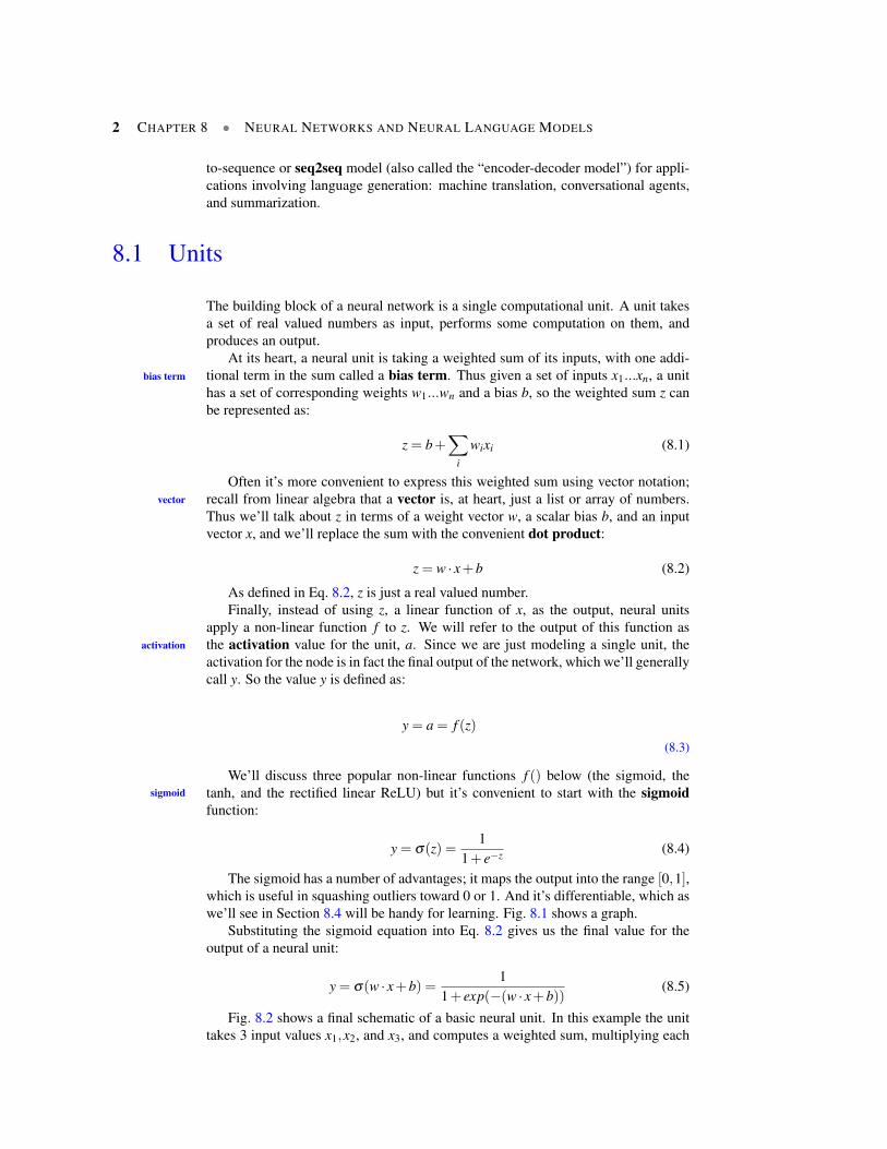
Fig. 8.2 shows a final schematic of a basic neural unit. In this example the unittakes 3 input values x1,x2, and x3, and computes a weighted sum, multiplying each

8.1 • UNITS 3

Figure 8.1 The sigmoid function takes a real value and maps it to the range [0,1]. Becauseit is nearly linear around 0 but has a sharp slope toward the ends, it tends to squash outliervalues toward 0 or 1.

value by a weight (w1, w2, and w3, respectively), adds them to a bias term b, and thenpasses the resulting sum through a sigmoid function to result in a number between 0and 1.

x1 x2 x3

y

w1 w2 w3

∑

b

σ

+1

z

a

Figure 8.2 A neural unit, taking 3 inputs x1, x2, and x3 (and a bias b that we represent as aweight for an input clamped at +1) and producing an output y. We include some convenientintermediate variables: the output of the summation, z, and the output of the sigmoid, a. Inthis case the output of the unit y is the same as a, but in deeper networks we’ll reserve y tomean the final output of the entire network, leaving a as the activation of an individual node.

Let’s walk through an example just to get an intuition. Let’s suppose we have aunit with the following weight vectors and bias:

w = [0.2,0.3,0.9]b = 0.5

What would this unit do with the following input vector:

x = [0.5,0.6,0.1]

4 CHAPTER 8 • NEURAL NETWORKS AND NEURAL LANGUAGE MODELS

The resulting output y would be:

y = σ(w · x+b) =1

1+ e−(w·x+b)=

11+ e−(.5∗.2+.3∗.6+.8∗.1+.5) = e−0.86 = .42

Other nonlinear functions besides the sigmoid are also commonly used. Thetanh function shown in Fig. 8.3a is a variant of the sigmoid that ranges from -1 totanh

+1:

y =ez− e−z

ez + e−z (8.6)

The simplest activation function is the rectified linear unit, also called the ReLU,ReLU

shown in Fig. 8.3b. It’s just the same as x when x is positive, and 0 otherwise:

y = max(x,0) (8.7)

(a) (b)

Figure 8.3 The tanh and ReLU activation functions.

These activation functions have different properties that make them useful fordifferent language applications or network architectures. For example the rectifierfunction has nice properties that result from it being very close to linear. In the sig-moid or tanh functions, very high values of z result in values of y that are saturated,saturated

i.e., extremely close to 1, which causes problems for learning. Rectifiers don’t havethis problem, since the output of values close to 1 also approaches 1 in a nice gentlelinear way. By contrast, the tanh function has the nice properties of being smoothlydifferentiable and mapping outlier values toward the mean.

8.2 The XOR problem

Early in the history of neural networks it was realized that the power of neural net-works, as with the real neurons that inspired them, comes from combining theseunits into larger networks.

One of the most clever demonstrations of the need for multi-layer networks wasthe proof by Minsky and Papert (1969) that a single neural unit cannot computesome very simple functions of its input. In the next section we take a look at thatintuition.

Consider the very simple task of computing simple logical functions of two in-puts, like AND, OR, and XOR. As a reminder, here are the truth tables for thosefunctions:

8.2 • THE XOR PROBLEM 5

AND OR XOR

x1 x2 y x1 x2 y x1 x2 y

0 0 0 0 0 0 0 0 0

0 1 0 0 1 1 0 1 1

1 0 0 1 0 1 1 0 1

1 1 1 1 1 1 1 1 0

This example was first shown for the perceptron, which is a very simple neuralperceptron

unit that has a binary output and no non-linear activation function. The output y ofa perceptron is 0 or 1, and just computed as follows (using the same weight w, inputx, and bias b as in Eq. 8.2):

y ={

0, if w · x+b≤ 01, if w · x+b > 0 (8.8)

It’s very easy to build a perceptron that can compute the logical AND and ORfunctions of its binary inputs; Fig. 8.4 shows the necessary weights.

x1

x2

+1-1

11

x1

x2

+10

11

(a) (b)

Figure 8.4 The weights w and bias b for perceptrons for computing logical functions. Theinputs are shown as x1 and x2 and the bias as a special node with value +1 which is multipliedwith the bias weight b. (a) logical AND, showing weights w1 = 1 and w2 = 1 and bias weightb = −1. (b) logical OR, showing weights w1 = 1 and w2 = 1 and bias weight b = 0. Theseweights/biases are just one from an infinite number of possible sets of weights and biases thatwould implement the functions.

It turns out, however, that it’s not possible to build a perceptron to computelogical XOR! (It’s worth spending a moment to give it a try!)

The intuition behind this important result relies on understanding that a percep-tron is a linear classifier. For a two-dimensional input x0 and x1, the perceptionequation, w1x1+w2x2+b = 0 is the equation of a line (we can see this by puttingit in the standard linear format: x2 =−(w1/w2)x1−b.) This line acts as a decisionboundary in two-dimensional space in which the output 0 is assigned to all inputsdecision

boundarylying on one side of the line, and the output 1 to all input points lying on the otherside of the line. If we had more than 2 inputs, the decision boundary becomes ahyperplane instead of a line, but the idea is the same, separating the space into twocategories.

Fig. 8.5 shows the possible logical inputs (00, 01, 10, and 11) and the line drawnby one possible set of parameters for an AND and an OR classifier. Notice that thereis simply no way to draw a line that separates the positive cases of XOR (01 and 10)from the negative cases (00 and 11). We say that XOR is not a linearly separablelinearly

separablefunction. Of course we could draw a boundary with a curve, or some other function,but not a single line.

6 CHAPTER 8 • NEURAL NETWORKS AND NEURAL LANGUAGE MODELS

00 1

1

x1

x2

00 1

1

x1

x2

00 1

1

x1

x2

a) x1 AND x2 b) x1 OR x2 c) x1 XOR x2

?

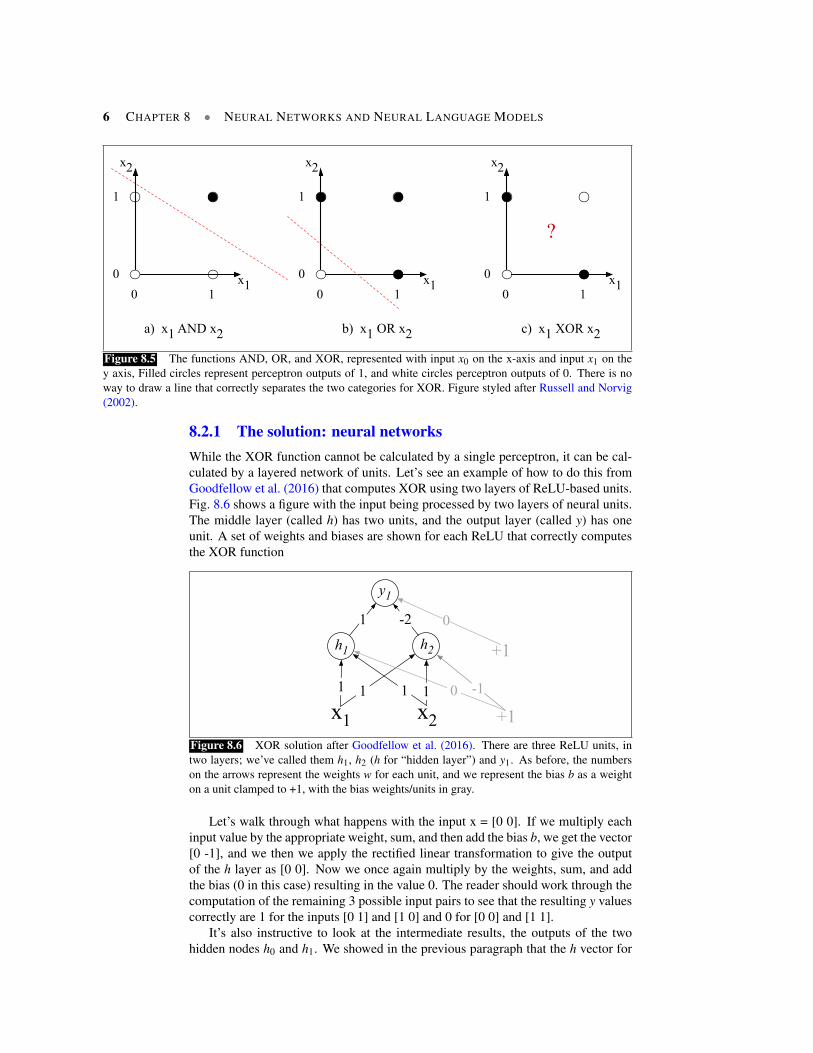
Figure 8.5 The functions AND, OR, and XOR, represented with input x0 on the x-axis and input x1 on they axis, Filled circles represent perceptron outputs of 1, and white circles perceptron outputs of 0. There is noway to draw a line that correctly separates the two categories for XOR. Figure styled after Russell and Norvig(2002).

8.2.1 The solution: neural networksWhile the XOR function cannot be calculated by a single perceptron, it can be cal-culated by a layered network of units. Let’s see an example of how to do this fromGoodfellow et al. (2016) that computes XOR using two layers of ReLU-based units.Fig. 8.6 shows a figure with the input being processed by two layers of neural units.The middle layer (called h) has two units, and the output layer (called y) has oneunit. A set of weights and biases are shown for each ReLU that correctly computesthe XOR function

x1 x2

h1 h2

y1

+1

1 -11 1

1 -2

01

+1

0

Figure 8.6 XOR solution after Goodfellow et al. (2016). There are three ReLU units, intwo layers; we’ve called them h1, h2 (h for “hidden layer”) and y1. As before, the numberson the arrows represent the weights w for each unit, and we represent the bias b as a weighton a unit clamped to +1, with the bias weights/units in gray.

Let’s walk through what happens with the input x = [0 0]. If we multiply eachinput value by the appropriate weight, sum, and then add the bias b, we get the vector[0 -1], and we then we apply the rectified linear transformation to give the outputof the h layer as [0 0]. Now we once again multiply by the weights, sum, and addthe bias (0 in this case) resulting in the value 0. The reader should work through thecomputation of the remaining 3 possible input pairs to see that the resulting y valuescorrectly are 1 for the inputs [0 1] and [1 0] and 0 for [0 0] and [1 1].

It’s also instructive to look at the intermediate results, the outputs of the twohidden nodes h0 and h1. We showed in the previous paragraph that the h vector for

8.3 • FEED-FORWARD NEURAL NETWORKS 7

the inputs x = [0 0] was [0 0]. Fig. 8.7b shows the values of the h layer for all 4inputs. Notice that hidden representations of the two input points x = [0 1] and x= [1 0] (the two cases with XOR output = 1) are merged to the single point h = [10]. The merger makes it easy to linearly separate the positive and negative casesof XOR. In other words, we can view the hidden layer of the network is forming arepresentation for the input.

0

0 1

1

x0

x1

a) The original x space

0

0 1

1

h0

h1

2

b) The new h space

Figure 8.7 The hidden layer forming a new representation of the input. Here is the rep-resentation of the hidden layer, h, compared to the original input representation x. Noticethat the input point [0 1] has been collapsed with the input point [1 0], making it possible tolinearly separate the positive and negative cases of XOR. After Goodfellow et al. (2016).

In this example we just stipulated the weights in Fig. 8.6. But for real exam-ples the weights for neural networks are learned automatically using the error back-propagation algorithm to be introduced in Section 8.4. That means the hidden layerswill learn to form useful representations. This intuition, that neural networks can au-tomatically learn useful representations of the input, is one of their key advantages,and one that we will return to again and again in later chapters.

Note that the solution to the XOR problem requires a network of units with non-linear activation functions. A network made up of simple linear (perceptron) unitscannot solve the XOR problem. This is because a network formed by many layersof purely linear units can always be reduced (shown to be computationally identicalto) a single layer of linear units with appropriate weights, and we’ve already shown(visually, in Fig. 8.5) that a single unit cannot solve the XOR problem.

8.3 Feed-Forward Neural Networks

Let’s now walk through a slightly more formal presentation of the simplest kind ofneural network, the feed-forward network. A feed-forward network is a multilayerfeed-forward

networknetwork in which the units are connected with no cycles; the outputs from units ineach layer are passed to units in the next higher layer, and no outputs are passedback to lower layers. (Later we’ll introduce networks with cycles, called recurrentneural networks.)

For historical reasons multilayer networks, especially feedforward networks, aresometimes called multi-layer perceptrons (or MLPs); this is a technical misnomer,multi-layer

perceptronsMLP since the units in modern multilayer networks aren’t perceptrons (perceptrons are

8 CHAPTER 8 • NEURAL NETWORKS AND NEURAL LANGUAGE MODELS

purely linear, but modern networks are made up of units with non-linearities likesigmoids), but at some point the name stuck.

Simple feed-forward networks have three kinds of nodes: input units, hiddenunits, and output units. Fig. 8.8 shows a picture.

x1 x2

h1 h2

y1

xdin…

h3hdh…

+1

b

…U

W

y2 ydout

Figure 8.8 Caption here

The input units are simply scalar values just as we saw in Fig. 8.2.The core of the neural network is the hidden layer formed of hidden units,hidden layer

each of which is a neural unit as described in Section 8.1, taking a weighted sum ofits inputs and then applying a non-linearity. In the standard architecture, each layeris fully-connected, meaning that each unit in each layer takes as input the outputsfully-connected

from all the units in the previous layer, and there is a link between every pair of unitsfrom two adjacent layers. Thus each hidden unit sums over all the input units.

Recall that a single hidden unit has parameters w (the weight vector) and b (thebias scalar). We represent the parameters for the entire hidden layer by combiningthe weight wi and bias bi for each unit i into a single weight matrix W and a singlebias vector b for the whole layer (see Fig. 8.8). Each element Wi j of the weightmatrix W represents the weight of the connection from the ith input unit xi to the thejth hidden unit h j.

The advantage of using a single matrix W for the weights of the entire layer isthat now that hidden layer computation for a feedforward network can be done veryefficiently with simple matrix operations. In fact, the computation only has threesteps: multiplying the weight matrix by the input vector x, adding the bias vector b,and applying the activation function f (such as the sigmoid, tanh, or rectified linearactivation function defined above).

The output of the hidden layer, the vector h, is thus the following, assuming thesigmoid function σ :

h = σ(Wx+b) (8.9)

Notice that we’re apply the σ function here to a vector, while in Eq. 8.4 it wasapplied to a scalar. We’re thus allowing σ(·), and indeed any activation functionf (·), to apply to a vector element-wise, so f [z1,z2,z3] = [ f (z1), f (z2), f (z3)].

Let’s introduce some constants to represent the dimensionalities of these vectorsand matrices. We’ll have din represent the number of inputs, so x is a vector ofreal numbers of dimensionality din, or more formally x ∈ Rdin . The hidden layer

8.3 • FEED-FORWARD NEURAL NETWORKS 9

has dimensional dh, so h ∈ Rdh and also b ∈ Rdh (since each hidden unit can take adifferent bias value). And the weight matrix W has dimensionality W ∈ Rdh×din .

Take a moment to convince yourself that the matrix multiplication in Eq. 8.9 willcompute the value of each hi j as

∑dini=1 wi jxi +b j.

As we saw in Section 8.2, the resulting value h (for hidden but also for hypoth-esis) forms a representation of the input. The role of the output layer is to takethis new representation h and compute a final output. This output could be a real-valued number, but in many cases the goal of the network is to make some sort ofclassification decision, and so we will focus on the case of classification.

If we are doing a binary task like sentiment classification, we might have a singleoutput node, and its value y is the probability of positive versus negative sentiment.If we are doing multinomial classification, such as assigning a part-of-speech tag, wemight have one output node for each potential part-of-speech, whose output valueis the probability of that part-of-speech, and the values of all the output nodes mustsum to one. The output layer thus gives a probability distribution across the outputnodes.

Let’s see how this happens. Like the hidden layer, the output layer has a weightmatrix (let’s call it U), but it often doesn’t have a bias vector b, so we’ll eliminateit in our examples here. The weight matrix is multiplied by the input vector (h) toproduce the intermediate output z.

z =Uh

There are dout output nodes, so z ∈ Rdout , weight matrix U has dimensionalityU ∈ Rdout×dh , and element Ui j is the weight from unit j in the hidden layer to unit iin the output layer.

However, z can’t be the output of the classifier, since it’s a vector of real-valuednumbers, while what we need for classification is a vector of probabilities. There isa convenient function for normalizing a vector of real values, by which we meannormalizing

converting it to a vector that encodes a probability distribution (all the numbers liebetween 0 and 1 and sum to 1): the softmax function.softmax

For a vector z of dimensionality D, the softmax is defined as:

softmax(zi) =ezi∑kj=1 ez j

1≤ i≤ D (8.10)

Thus for example given a vector z=[0.6 1.1 -1.5 1.2 3.2 -1.1], softmax(z) is [0.055 0.090 0.0067 0.10 0.74 0.010].

You may recall that softmax was exactly what is used to create a probability dis-tribution from a vector of real-valued numbers (computed from summing weightstimes features) in logistic regression in Chapter 7; the equation for computing theprobability of y being of class c given x in multinomial logistic regression was (re-peated from Eq. 8.11):

p(c|x) =

exp

(N∑

i=1

wi fi(c,x)

)∑c′∈C

exp

(N∑

i=1

wi fi(c′,x)

) (8.11)

10 CHAPTER 8 • NEURAL NETWORKS AND NEURAL LANGUAGE MODELS

In other words, we can think of a neural network classifier with one hidden layeras building a vector h which is a hidden layer representation of the input, and thenrunning standard logistic regression on the features that the network develops in h.By contrast, in Chapter 7 the features were mainly designed by hand via featuretemplates. So a neural network is like logistic regression, but (a) with many layers,since a deep neural network is like layer after layer of logistic regression classifiers,and (b) rather than forming the features by feature templates, the prior layers of thenetwork induce the feature representations themselves.

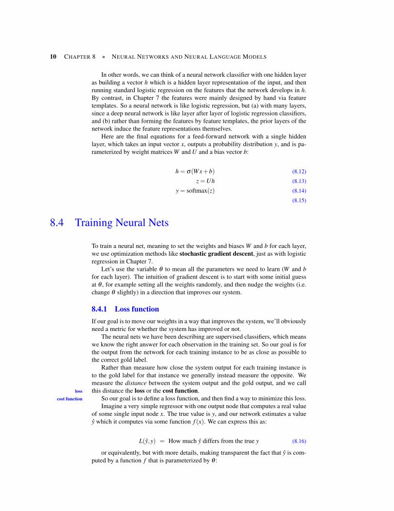
Here are the final equations for a feed-forward network with a single hiddenlayer, which takes an input vector x, outputs a probability distribution y, and is pa-rameterized by weight matrices W and U and a bias vector b:

h = σ(Wx+b) (8.12)

z =Uh (8.13)

y = softmax(z) (8.14)

(8.15)

8.4 Training Neural Nets

To train a neural net, meaning to set the weights and biases W and b for each layer,we use optimization methods like stochastic gradient descent, just as with logisticregression in Chapter 7.

Let’s use the variable θ to mean all the parameters we need to learn (W and bfor each layer). The intuition of gradient descent is to start with some initial guessat θ , for example setting all the weights randomly, and then nudge the weights (i.e.change θ slightly) in a direction that improves our system.

8.4.1 Loss functionIf our goal is to move our weights in a way that improves the system, we’ll obviouslyneed a metric for whether the system has improved or not.

The neural nets we have been describing are supervised classifiers, which meanswe know the right answer for each observation in the training set. So our goal is forthe output from the network for each training instance to be as close as possible tothe correct gold label.

Rather than measure how close the system output for each training instance isto the gold label for that instance we generally instead measure the opposite. Wemeasure the distance between the system output and the gold output, and we callthis distance the loss or the cost function.loss

cost function So our goal is to define a loss function, and then find a way to minimize this loss.Imagine a very simple regressor with one output node that computes a real value

of some single input node x. The true value is y, and our network estimates a valuey which it computes via some function f (x). We can express this as:

L(y,y) = How much y differs from the true y (8.16)

or equivalently, but with more details, making transparent the fact that y is com-puted by a function f that is parameterized by θ :

8.4 • TRAINING NEURAL NETS 11

L( f (x;θ),y) = How much f (x) differs from the true y (8.17)

A common loss function for such a network (or for the similar case of linearregression) is the mean-squared error or MSE between the true value y(i) and themean-squared

errorMSE system’s output y(i), the average over the m observations of the square of the error in

y for each one:

LMSE(y,y) =1n

m∑i=1

(y(m)− y(i))2 (8.18)

While mean squared error makes sense for regression tasks, mostly in this chap-ter we have been considering nets as probabilistic classifiers. For probabilistic classi-fiers a common loss function—also used in training logistic regression—is the crossentropy loss, also called the negative log likelihood. Let y be a vector over the Ccross entropy

lossclasses representing the true output probability distribution. Assume this is a hardclassification task, meaning that only one class is the correct one. If the true classis i, then y is a vector where yi = 1 and y j = 0 ∀ j 6= i. A vector like this, with onevalue=1 and the rest 0, is called a one-hot vector. Now let y be the vector outputfrom the network. The loss is simply the log probability of the correct class:

L(y,y) =− log p(yi) (8.19)

Why the negative log probability? A perfect classifier would assign the correctclass i probability 1 and all the incorrect classes probability 0. That means the higherp(yi) (the closer it is to 1), the better the classifier; p(yi) is (the closer it is to 0), theworse the classifier. The negative log of this probability is a beautiful loss metricsince it goes from 0 (negative log of 1, no loss) to infinity (negative log of 0, infiniteloss). This loss function also insures that as probability of the correct answer ismaximized, the probability of all the incorrect answers is minimized; since they allsum to one, any increase in the probability of the correct answer is coming at theexpense of the incorrect answers.

Given a loss function1 our goal in training is to move the parameters so as tominimize the loss, finding the minimum of the loss function.

8.4.2 Following GradientsHow shall we find the minimum of this loss function? Gradient descent is a methodthat finds a minimum of a function by figuring out in which direction (in the spaceof the parameters θ ) the function’s slope is rising the most steeply, and moving inthe opposite direction.

The intuition is that if you are hiking the Grand Canyon and trying to descendmost quickly down to the river you might look around yourself 360 degrees, findthe direction where the ground is sloping the steepest, and walk downhill in thatdirection.

Although the algorithm (and the concept of gradient) are designed for directionvectors, let’s first consider a visualization of the the case where, θ , the parameter ofour system, is just a single scalar, shown in Fig. 8.9.

Given a random initialization of θ at some value θ1, and assuming the loss func-tion L happened to have the shape in Fig. 8.9, we need the algorithm to tell us

1 See any machine learning textbook for lots of other potential functions like the useful hinge loss.

12 CHAPTER 8 • NEURAL NETWORKS AND NEURAL LANGUAGE MODELS

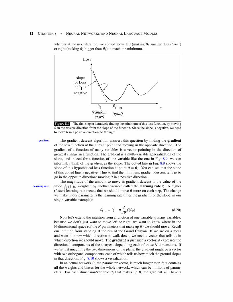
whether at the next iteration, we should move left (making θ2 smaller than theta1)or right (making θ2 bigger than θ1) to reach the minimum.

θ

Loss

(random start)

θ1 θmin

slopeof Lossat θ1 is

negative

(goal)

Figure 8.9 The first step in iteratively finding the minimum of this loss function, by movingθ in the reverse direction from the slope of the function. Since the slope is negative, we needto move θ in a positive direction, to the right.

The gradient descent algorithm answers this question by finding the gradientgradient

of the loss function at the current point and moving in the opposite direction. Thegradient of a function of many variables is a vector pointing in the direction ofgreatest change in a function. The gradient is a multi-variable generalization of theslope, and indeed for a function of one variable like the one in Fig. 8.9, we caninformally think of the gradient as the slope. The dotted line in Fig. 8.9 shows theslope of this hypothetical loss function at point θ = θ0. You can see that the slopeof this dotted line is negative. Thus to find the minimum, gradient descent tells us togo in the opposite direction: moving θ in a positive direction.

The magnitude of the amount to move in gradient descent is the value of theslope d

dθf (θ0) weighted by another variable called the learning rate η . A higherlearning rate

(faster) learning rate means that we should move θ more on each step. The changewe make in our parameter is the learning rate times the gradient (or the slope, in oursingle-variable example):

θt+1 = θt −ηd

dθf (θ0) (8.20)

Now let’s extend the intuition from a function of one variable to many variables,because we don’t just want to move left or right, we want to know where in theN-dimensional space (of the N parameters that make up θ ) we should move. Recallour intuition from standing at the rim of the Grand Canyon. If we are on a mesaand want to know which direction to walk down, we need a vector that tells us inwhich direction we should move. The gradient is just such a vector; it expresses thedirectional components of the sharpest slope along each of those N dimensions. Ifwe’re just imagining the two dimensions of the plane, the gradient might be a vectorwith two orthogonal components, each of which tells us how much the ground slopesin that direction. Fig. 8.10 shows a visualization:

In an actual network θ , the parameter vector, is much longer than 2; it containsall the weights and biases for the whole network, which can be millions of param-eters. For each dimension/variable θ j that makes up θ , the gradient will have a

8.4 • TRAINING NEURAL NETS 13

Figure 8.10 Visualization of the gradient vector in two dimensions.

component that tells us the slope with respect to that variable. Essentially we’re ask-ing: “How much would a small change in that variable θ j influence the loss functionL?”

In each dimension θ j, we express the slope as a partial derivative ∂

∂θ jof the loss

function. The gradient is then defined as a vector of these partials:

∇θ L( f (x;θ),y)) =

∂

∂θ1L( f (x;θ),y)

∂

∂θ2L( f (x;θ),y)

...∂

∂θmL( f (x;θ),y)

(8.21)

The final equation for updating θ based on the gradient is thus

θt+1 = θt −η∇L( f (x;θ),y) (8.22)

8.4.3 Computing the GradientComputing the gradient requires the partial derivative of the loss function with re-spect to each parameter. This can be complex for deep networks, where we arecomputing the derivative with respect to weight parameters that appear all the wayback in the very early layers of the network, even though the loss is computed onlyat the very end of the network.

The solution to computing this gradient is known as error backpropagationerror back-propagation

or backprop (Rumelhart et al., 1986), which turns out to be a special case of back-ward differentiation. In backprop, the loss function is first modeled as a computationgraph, in which each edge is a computation and each node the result of the compu-tation. The chain rule of differentiation is then used to annotate this graph with thepartial derivatives of the loss function along each edge of the graph. We give a briefoverview of the algorithm in the next subsections; further details can be found in anymachine learning or data-intensive computation textbook.

Computation Graphs

TBD

14 CHAPTER 8 • NEURAL NETWORKS AND NEURAL LANGUAGE MODELS

Error Back Propagation

TBD

8.4.4 Stochastic Gradient DescentOnce we have computed the gradient, we can use it to train θ . The stochastic gradi-ent descent algorithm (LeCun et al., 2012) is an online algorithm that computes thisgradient after each training example, and nudges θ in the right direction. Fig. 8.11shows the algorithm.

function STOCHASTIC GRADIENT DESCENT(L(), f (), x, y) returns θ

# where: L is the loss function# f is a function parameterized by θ

# x is the set of training inputs x(1), x(2), ..., x(n)

# y is the set of training outputs (labels) y(1), y(2), ..., y(n)

θ←small random valueswhile not done

Sample a training tuple (x(i), y(i))Compute the loss L( f (x(i);θ),y(i)) # How far off is f (x(i)) from y(i)?g←∇θ L( f (x(i);θ),y(i)) # How should we move θ to maximize loss ?θ←θ − ηk g # go the other way instead

Figure 8.11 The stochastic gradient descent algorithm, after (Goldberg, 2017).

Stochastic gradient descent is called stochastic because it chooses a single ran-dom example at a time, moving the weights so as to improve performance on thatsingle example. That can result in very choppy movements, so an alternative versionof the algorithm, minibatch gradient descent, computes the gradient over batches ofminibatch

training instances rather than a single instance.The learning rate ηk is a parameter that must be adjusted. If it’s too high, the

learner will take steps that are too large, overshooting the minimum of the loss func-tion. If it’s too low, the learner will take steps that are too small, and take too long toget to the minimum. It is most common to being the learning rate at a higher value,and then slowly decrease it, so that it is a function of the iteration k of training.

8.5 Neural Language Models

Now that we’ve introduced neural networks it’s time to see an application. The firstapplication we’ll consider is language modeling: predicting upcoming words fromprior word context.

Although we have already introduced a perfectly useful language modeling paradigm(the smoothed N-grams of Chapter 4), neural net-based language models turn out tohave many advantages. Among these are that neural language models don’t needsmoothing, they can handle much longer histories, and they can generalize overcontexts of similar words. Furthermore, neural net language models underlie manyof the models we’ll introduce for generation, summarization, machine translation,and dialog.

8.5 • NEURAL LANGUAGE MODELS 15

On the other hand, there is a cost for this improved performance: neural netlanguage models are strikingly slower to train than traditional language models, andso for many tasks traditional language modeling is still the right technology.

In this chapter we’ll describe simple feedforward neural language models, firstintroduced by Bengio et al. (2003). We will turn to the recurrent language model,more commonly used today, in Chapter 9b.

A feedforward neural LM is a standard feedforward network that takes as inputat time t a representation of some number of previous words (wt−1,wt−2, etc) andoutputs a probability distribution over possible next words. Thus, like the traditionalLM the feedforward neural LM approximates the probability of a word given theentire prior context P(wt |wt−1

1 ) by approximating based on the N previous words:

P(wt |wt−11 )≈ P(wt |wt−1

t−N+1) (8.23)

In the following examples we’ll use a 4-gram example, so we’ll show a net toestimate the probability P(wt = i|wt−1,wt−2,wt−3).

8.5.1 EmbeddingsThe insight of neural language models is in how to represent the prior context. Eachword is represented as a vector of real numbers of of dimension d; d tends to liebetween 50 and 500, depending on the system. These vectors for each words arecalled embeddings, because we represent a word as being embedded in a vectorembeddings

space. By contrast, in many traditional NLP applications, a word is represented as astring of letters, or an index in a vocabulary list.

Why represent a word as a vector of 50 numbers? Vectors turn out to be areally powerful representation for words, because a distributed representation allowswords that have similar meanings, or similar grammatical properties, to have similarvectors. As we’ll see in Chapter 15, embedding that are learned for words like“cat” and “dog”— words with similar meaning and parts of speech—will be similarvectors. That will allow us to generalize our language models in ways that wasn’tpossible with traditional N-gram models.

For example, suppose we’ve seen this sentence in training:

I have to make sure when I get home to feed the cat.

and then in our test set we are trying to predict what comes after the prefix “I forgotwhen I got home to feed the”.

A traditional N-gram model will predict “cat”. But suppose we’ve never seenthe word “dog” after the words ”feed the”. A traditional LM won’t expect “dog”.But by representing words as vectors, and assuming the vector for “cat” is similar tothe vector for “dog”, a neural LM, even if it’s never seen “feed the dog”, will assigna reasonably high probability to “dog” as well as “cat”, merely because they havesimilar vectors.

Representing words as embeddings vectors is central to modern natural languageprocessing, and is generally referred to as the vector space model of meaning. Wewill go into lots of details on the different kinds of embeddings in Chapter 15 andChapter 152.

Let’s set aside—just for a few pages—the question of how these embeddingsare learned. Imagine that we had an embedding dictionary E that gives us, for eachword in our vocabulary V , the vector for that word.

Fig. 8.12 shows a sketch of this simplified FFNNLM with N=3; we have a mov-ing window at time t with a one-hot vector representing each of the 3 previous words

16 CHAPTER 8 • NEURAL NETWORKS AND NEURAL LANGUAGE MODELS

(words wt−1, wt−2, and wt−3). These 3 vectors are concatenated together to producex, the input layer of a neural network whose output is a softmax with a probabilitydistribution over words. Thus y42, the value of output node 42 is the probability ofthe next word wt being V42, the vocabulary word with index 42.

h1 h2

y1

h3 hdh…

…

U

W

y42 y|V|

Projection layer 1⨉3dconcatenated embeddings

for context words

Hidden layer

Output layer P(w|u) …

in thehole... ...ground there lived

word 42embedding for

word 35embedding for

word 9925embedding for

word 45180

wt-1wt-2 wtwt-3

dh⨉3d

1⨉dh

|V|⨉dh P(wt=V42|wt-3,wt-2,wt-3)

1⨉|V|

Figure 8.12 A simplified view of a feedforward neural language model moving through a text. At eachtimestep t the network takes the 3 context words, converts each to a d-dimensional embeddings, and concate-nates the 3 embeddings together to get the 1×Nd unit input layer x for the network. These units are multipliedby a weight matrix W and bias vector b and then an activation function to produce a hidden layer h, which isthen multiplied by another weight matrix U . (For graphic simplicity we don’t show b in this and future pictures).Finally, a softmax output layer predicts at each node i the probability that the next word wt will be vocabularyword Vi. (This picture is simplified because it assumes we just look up in a dictionary table E the “embeddingvector”, a d-dimensional vector representing each word, but doesn’t yet show us how these embeddings arelearned.)

The model shown in Fig. 8.12 is quite sufficient, assuming we learn the em-beddings separately by a method like the word2vec methods of Chapter 152. Themethod of using another algorithm to learn the embedding representations we usefor input words is called pretraining. If those pretrained embeddings are sufficientpretraining

for your purposes, then this is all you need.However, often we’d like to learn the embeddings simultaneously with training

the network. This is true when whatever task the network is designed for (sentimentclassification, or translation, or parsing) places strong constraints on what makes agood representation.

Let’s therefore show an architecture that allows the embeddings to be learned.To do this, we’ll add an extra layer to the network, and propagate the error all theway back to the embedding vectors, starting with embeddings with random valuesand slowly moving toward sensible representations.

For this to work at the input layer, instead of pre-trained embeddings, we’regoing to represent each of the N previous words as a one-hot vector of length |V |, i.e.,with one dimension for each word in the vocabulary. A one-hot vector is a vectorone-hot vector

that has one element equal to 1—in the dimension corresponding to that word’sindex in the vocabulary— while all the other elements are set to zero.

8.5 • NEURAL LANGUAGE MODELS 17

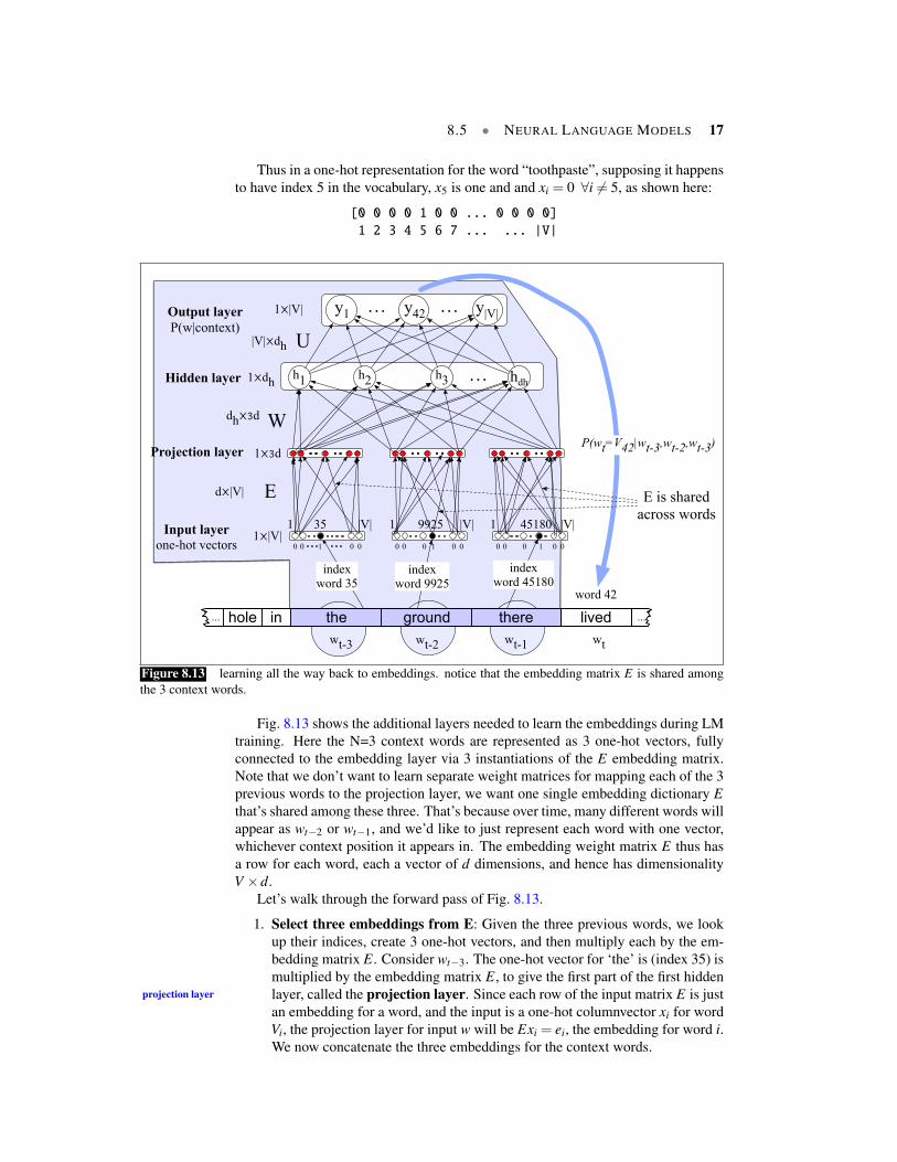
Thus in a one-hot representation for the word “toothpaste”, supposing it happensto have index 5 in the vocabulary, x5 is one and and xi = 0 ∀i 6= 5, as shown here:

[0 0 0 0 1 0 0 ... 0 0 0 0]

1 2 3 4 5 6 7 ... ... |V|

h1 h2

y1

h3 hdh…

…

U

W

y42 y|V|

Projection layer 1⨉3d

Hidden layer

Output layer P(w|context)

…

in thehole... ...ground there lived

word 42

wt-1wt-2 wtwt-3

dh⨉3d

1⨉dh

|V|⨉dh

P(wt=V42|wt-3,wt-2,wt-3)

1⨉|V|

Input layerone-hot vectors

indexword 35

0 0 1 00

1 |V|35

0 0 1 00

1 |V|45180

0 0 1 00

1 |V|9925

0 0

index word 9925

index word 45180

E

1⨉|V|

d⨉|V| E is sharedacross words

Figure 8.13 learning all the way back to embeddings. notice that the embedding matrix E is shared amongthe 3 context words.

Fig. 8.13 shows the additional layers needed to learn the embeddings during LMtraining. Here the N=3 context words are represented as 3 one-hot vectors, fullyconnected to the embedding layer via 3 instantiations of the E embedding matrix.Note that we don’t want to learn separate weight matrices for mapping each of the 3previous words to the projection layer, we want one single embedding dictionary Ethat’s shared among these three. That’s because over time, many different words willappear as wt−2 or wt−1, and we’d like to just represent each word with one vector,whichever context position it appears in. The embedding weight matrix E thus hasa row for each word, each a vector of d dimensions, and hence has dimensionalityV ×d.

Let’s walk through the forward pass of Fig. 8.13.

1. Select three embeddings from E: Given the three previous words, we lookup their indices, create 3 one-hot vectors, and then multiply each by the em-bedding matrix E. Consider wt−3. The one-hot vector for ‘the’ is (index 35) ismultiplied by the embedding matrix E, to give the first part of the first hiddenlayer, called the projection layer. Since each row of the input matrix E is justprojection layer

an embedding for a word, and the input is a one-hot columnvector xi for wordVi, the projection layer for input w will be Exi = ei, the embedding for word i.We now concatenate the three embeddings for the context words.

18 CHAPTER 8 • NEURAL NETWORKS AND NEURAL LANGUAGE MODELS

2. Multiply by W: We now multiply by W (and add b) and pass through therectified linear (or other) activation function to get the hidden layer h.

3. Multiply by U: h is now multiplied by U4. Apply softmax: After the softmax, each node i in the output layer estimates

the probability P(wt = i|wt−1,wt−2,wt−3)

In summary, if we use e to represent the projection layer, formed by concatenat-ing the 3 embedding for the three context vectors, the equations for a neural languagemodel become:

e = (Ex1,Ex2, ...,Ex) (8.24)

h = σ(We+b) (8.25)

z =Uh (8.26)

y = softmax(z) (8.27)

8.5.2 Training the neural language modelTo train the model, i.e. to set all the parameters θ = E,W,U,b, we use the SGD al-gorithm of Fig. 8.11, with error back propagation to compute the gradient. Trainingthus not only sets the weights W and U of the network, but also as we’re predictingupcoming words, we’re learning the embeddings E for each words that best predictupcoming words.

Generally training proceedings by taking as input a very long text, concatenatingall the sentences, start with random weights, and then iteratively moving through thetext predicting each word wt . At each word wt , the categorial cross-entropy (negativelog likelihood) loss is:

L =− log p(wt |wt−1, ...,wt−n+1) (8.28)

The gradient is computed for this loss by differentiation:

θt+1 = θt −η∂ log p(wt |wt−1, ...,wt−n+1)

∂θ(8.29)

And then backpropagated through U , W , b, E.

8.6 Summary

• Neural networks are built out of neural units, originally inspired by humanneurons but now simple an abstract computational device.

• Each neural unit multiplies input values by a weight vector, adds a bias, andthen applies a non-linear activation function like sigmoid, tanh, or rectifiedlinear.

• In a fully-connected, feedforward network, each unit in layer i is connectedto each unit in layer i+1, and there are no cycles.

• The power of neural networks comes from the ability of early layers to learnrepresentations that can be utilized by later layers in the network.

• Neural networks are trained by optimization algorithms like stochastic gra-dient descent.

BIBLIOGRAPHICAL AND HISTORICAL NOTES 19

• Error back propagation is used to compute the gradients of the loss functionfor a network.

• Neural language modeling uses a network as a probabilistic classifier, tocompute the probability of the next word given the previous N word.

• Neural language models make use of embeddings, dense vectors of between50 and 500 dimensions that represent words in the input vocabulary.

Bibliographical and Historical NotesThe origins of neural networks lie in the 1940s McCulloch-Pitts neuron (McCul-loch and Pitts, 1943), a simplified model of the human neuron as a kind of com-puting element that could be described in terms of propositional logic. By the late1950s and early 1960s, a number of labs (including Frank Rosenblatt at Cornell andBernard Widrow at Stanford) developed research into neural networks; this phasesaw the development of the perceptron (Rosenblatt, 1958), and the transformationof the threshold into a bias, a notation we still use (Widrow and Hoff, 1960).

The field of neural networks declined after it was shown that a single perceptronunit was unable to model functions as simple as XOR (Minsky and Papert, 1969).While some small amount of work continued during the next two decades, a majorrevival for the field didn’t come until the 1980s, when practical tools for buildingdeeper networks like error back propagation became widespread (Rumelhart et al.,1986). During the 1980s a wide variety of neural network and related architectureswere developed, particularly for applications in psychology and cognitive science(Rumelhart and McClelland 1986b, McClelland and Elman 1986, Rumelhart andMcClelland 1986a,Elman 1990), for which the term connectionist or parallel dis-connectionist

tributed processing was often used (Feldman and Ballard 1982, Smolensky 1988).Many of the principles and techniques developed in this period are foundationalto modern work, including the idea of distributed representations (Hinton, 1986),of recurrent networks (Elman, 1990), and the use of tensors for compositionality(Smolensky, 1990).

By the 1990s larger neural networks began to be applied to many practical lan-guage processing tasks as well, like handwriting recognition (LeCun et al. 1989,LeCun et al. 1990) and speech recognition (Morgan and Bourlard 1989, Morganand Bourlard 1990). By the early 2000s, improvements in computer hardware andadvances in optimization and training techniques made it possible to train even largerand deeper networks, leading to the modern term deep learning (Hinton et al. 2006,Bengio et al. 2007). We cover more related history in Chapter 9b.

There are a number of excellent books on the subject. Goldberg (2017) has asuperb and comprehensive coverage of neural networks for natural language pro-cessing. For neural networks in general see Goodfellow et al. (2016) and Nielsen(2015).

The description in this chapter has been quite high-level, and there are manydetails of neural network training and architecture that are necessary to successfullytrain models. For example various forms of regularization are used to prevent over-fitting, including dropout: randomly dropping some units and their conntectionsdropout

from the network during training (Hinton et al. 2012, Srivastava et al. 2014). Fasteroptimization methods than vanilla stochastic gradient descent are often used, suchas Adam (Kingma and Ba, 2015).

20 CHAPTER 8 • NEURAL NETWORKS AND NEURAL LANGUAGE MODELS

Since neural networks training and decoding require significant numbers of vec-tor operations, modern systems are often trained using vector-based GPUs (GraphicProcessing Units). A number of software engineering tools are widely availableincluding TensorFlow (Abadi et al., 2015) and others.

Bibliographical and Historical Notes 21

Abadi, M., Agarwal, A., Barham, P., Brevdo, E., Chen, Z.,Citro, C., Corrado, G. S., Davis, A., Dean, J., Devin, M.,Ghemawat, S., Goodfellow, I., Harp, A., Irving, G., Isard,M., Jia, Y., Jozefowicz, R., Kaiser, L., Kudlur, M., Lev-enberg, J., Mane, D., Monga, R., Moore, S., Murray, D.,Olah, C., Schuster, M., Shlens, J., Steiner, B., Sutskever,I., Talwar, K., Tucker, P., Vanhoucke, V., Vasudevan, V.,Viegas, F., Vinyals, O., Warden, P., Wattenberg, M., Wicke,M., Yu, Y., and Zheng, X. (2015). TensorFlow: Large-scale machine learning on heterogeneous systems.. Soft-ware available from tensorflow.org.

Bengio, Y., Ducharme, R., Vincent, P., and Jauvin, C. (2003).A neural probabilistic language model. Journal of machinelearning research, 3(Feb), 1137–1155.

Bengio, Y., Lamblin, P., Popovici, D., and Larochelle, H.(2007). Greedy layer-wise training of deep networks. InNIPS 2007, pp. 153–160.

Elman, J. L. (1990). Finding structure in time. Cognitivescience, 14(2), 179–211.

Feldman, J. A. and Ballard, D. H. (1982). Connectionistmodels and their properties. Cognitive Science, 6, 205–254.

Goldberg, Y. (2017). Neural Network Methods for NaturalLanguage Processing, Vol. 10 of Synthesis Lectures on Hu-man Language Technologies. Morgan & Claypool.

Goodfellow, I., Bengio, Y., and Courville, A. (2016). DeepLearning. MIT Press.

Hinton, G. E. (1986). Learning distributed representationsof concepts. In COGSCI-86, pp. 1–12.

Hinton, G. E., Osindero, S., and Teh, Y.-W. (2006). A fastlearning algorithm for deep belief nets. Neural computa-tion, 18(7), 1527–1554.

Hinton, G. E., Srivastava, N., Krizhevsky, A., Sutskever,I., and Salakhutdinov, R. R. (2012). Improving neuralnetworks by preventing co-adaptation of feature detectors.arXiv preprint arXiv:1207.0580.

Kingma, D. and Ba, J. (2015). Adam: A method for stochas-tic optimization. In ICLR 2015.

LeCun, Y., Boser, B., Denker, J. S., Henderson, D., Howard,R. E., Hubbard, W., and Jackel, L. D. (1989). Backpropa-gation applied to handwritten zip code recognition. Neuralcomputation, 1(4), 541–551.

LeCun, Y., Boser, B. E., Denker, J. S., Henderson, D.,Howard, R. E., Hubbard, W. E., and Jackel, L. D. (1990).Handwritten digit recognition with a back-propagation net-work. In NIPS 1990, pp. 396–404.

LeCun, Y. A., Bottou, L., Orr, G. B., and Muller, K.-R.(2012). Efficient backprop. In Neural networks: Tricksof the trade, pp. 9–48. Springer.

McClelland, J. L. and Elman, J. L. (1986). The TRACEmodel of speech perception. Cognitive Psychology, 18, 1–86.

McCulloch, W. S. and Pitts, W. (1943). A logical calculus ofideas immanent in nervous activity. Bulletin of Mathemat-ical Biophysics, 5, 115–133. Reprinted in Neurocomput-ing: Foundations of Research, ed. by J. A. Anderson and ERosenfeld. MIT Press 1988.

Minsky, M. and Papert, S. (1969). Perceptrons. MIT Press.

Morgan, N. and Bourlard, H. (1989). Generalization and pa-rameter estimation in feedforward nets: Some experiments.In Advances in neural information processing systems, pp.630–637.

Morgan, N. and Bourlard, H. (1990). Continuous speechrecognition using multilayer perceptrons with hiddenmarkov models. In ICASSP-90, pp. 413–416.

Nielsen, M. A. (2015). Neural networks and Deep learning.Determination Press USA.

Rosenblatt, F. (1958). The perceptron: A probabilistic modelfor information storage and organization in the brain.. Psy-chological review, 65(6), 386–408.

Rumelhart, D. E., Hinton, G. E., and Williams, R. J. (1986).Learning internal representations by error propagation. InRumelhart, D. E. and McClelland, J. L. (Eds.), ParallelDistributed Processing, Vol. 2, pp. 318–362. MIT Press.

Rumelhart, D. E. and McClelland, J. L. (1986a). On learn-ing the past tense of English verbs. In Rumelhart, D. E. andMcClelland, J. L. (Eds.), Parallel Distributed Processing,Vol. 2, pp. 216–271. MIT Press.

Rumelhart, D. E. and McClelland, J. L. (Eds.). (1986b). Par-allel Distributed Processing. MIT Press.

Russell, S. and Norvig, P. (2002). Artificial Intelligence: AModern Approach (2nd Ed.). Prentice Hall.

Smolensky, P. (1988). On the proper treatment of connec-tionism. Behavioral and brain sciences, 11(1), 1–23.

Smolensky, P. (1990). Tensor product variable binding andthe representation of symbolic structures in connectionistsystems. Artificial intelligence, 46(1-2), 159–216.

Srivastava, N., Hinton, G. E., Krizhevsky, A., Sutskever, I.,and Salakhutdinov, R. (2014). Dropout: a simple way toprevent neural networks from overfitting.. Journal of Ma-chine Learning Research, 15(1), 1929–1958.

Widrow, B. and Hoff, M. E. (1960). Adaptive switching cir-cuits. In IRE WESCON Convention Record, Vol. 4, pp.96–104.