CHAPTER Strength of Materials This chapter reviews concepts of strength of materials (also known as mechanics of materials). The methods to calculate stresses and strains for various types of loading are a necessary precursor to the process of structural design, wherein those calculated maximum stresses are checked against allowable stresses (allowable stress design). Exter- nal loads imposed on structures produce internal loads such as axial force (normal to cross section), transverse shear force (in the plane of the cross section), bending moment (about major and minor in-plane axes), and torsion (moment about the axis normal to the cross section). The externally imposed loads and the internal loads are in equilibrium. These internal loads are then responsible for creating internal stresses such as normal stress and shear stress. Sign Convention for Stresses The naming convention for stress components on a 3D element uses two subscripts—the first indicating the plane on which the stress component acts and the second indicating the direction of the stress component. Thus, τ xy indicates the (shear) stress component acting on the x-face (face whose outward normal is in the x direction, or a face parallel to the yz plane). In Fig. 101.1, this face is shown shaded. In three dimensions, there are three normal stress components (σ xx , σ yy , and σ zz ) while there are six shear stress components (τ xy , τ yx , τ xz , τ zx , τ yz , τ zy ). It can be shown that τ xy = τ yx , τ xz = τ zx , τ yz = τ zy , which leaves only six independent stress components: three normal (σ xx , σ yy , σ zz ) and three shear (τ xy , τ xz , τ yz ). The stress components on the x-plane are shown in Fig. 101.1. This chapter reviews computation of internal normal and shear stress produced by axial load, normal and shear stress produced by transverse loads, and shear stress pro- duced by torsion. In addition, the membrane stresses produced by internal pressure in thick- and thin-walled pressure vessels are also reviewed. 101 1
Transcript
CHAPTER
Strength of Materials
This chapter reviews concepts of strength of materials (also known as mechanics of materials). The methods to calculate stresses and strains for various types of loading are a necessary precursor to the process of structural design, wherein those calculated maximum stresses are checked against allowable stresses (allowable stress design). Exter-nal loads imposed on structures produce internal loads such as axial force (normal to cross section), transverse shear force (in the plane of the cross section), bending moment (about major and minor in-plane axes), and torsion (moment about the axis normal to the cross section). The externally imposed loads and the internal loads are in equilibrium. These internal loads are then responsible for creating internal stresses such as normal stress and shear stress.
Sign Convention for StressesThe naming convention for stress components on a 3D element uses two subscripts—the first indicating the plane on which the stress component acts and the second indicating the direction of the stress component. Thus, τ
xy indicates the (shear) stress component
acting on the x-face (face whose outward normal is in the x direction, or a face parallel to the yz plane). In Fig. 101.1, this face is shown shaded. In three dimensions, there are three normal stress components (σ
xx, σ
yy, and σ
zz) while there are six shear stress
components (τxy, τ
yx, τ
xz, τ
zx, τ
yz, τ
zy). It can be shown that τ
xy = τyx , τ
xz = τzx, τ
yz = τzy, which
leaves only six independent stress components: three normal (σxx
, σyy , σ
zz) and three
shear (τxy, τ
xz, τ
yz). The stress components on the x-plane are shown in Fig. 101.1.
This chapter reviews computation of internal normal and shear stress produced by axial load, normal and shear stress produced by transverse loads, and shear stress pro-duced by torsion. In addition, the membrane stresses produced by internal pressure in thick- and thin-walled pressure vessels are also reviewed.
Centroid of an Area by IntegrationThe center of gravity of any object is calculated as the weighted average of the centers of gravity of subobjects that constitute the object. When the area is subdivided into infinitesimal elements, this weighted average is calculated by integration. For an area, the location of the centroid (x
c, y
c) is given by
xxdA
dAy
ydA
dAc c= =∫
∫∫∫
(101.1)
where x and y represent the coordinates of the center of the element dA being integrated.
NOTE Practical applications where the centroid location needs to be calculated, e.g., to find section properties of certain built-up shapes, the shape is often composed of geometrically well-known parts. In that case, the weighted average of these parts can be computed, rather than the much more complex integration approach.
Centroid of a Compound Area—Weighted AverageWhen one is dealing with a compound shape (which is a combination of a finite number of known shapes), the composite formula may be applied. The coordinates of the centroid are given by the weighted average of the coordinates of individual parts:
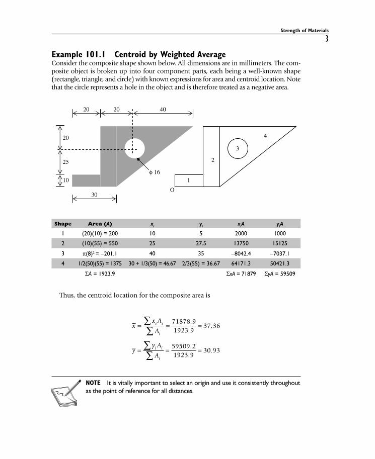
Example 101.1 Centroid by Weighted AverageConsider the composite shape shown below. All dimensions are in millimeters. The com-posite object is broken up into four component parts, each being a well-known shape (rectangle, triangle, and circle) with known expressions for area and centroid location. Note that the circle represents a hole in the object and is therefore treated as a negative area.
The in-plane axes passing through the geometric centroid are also called the elastic neutral axes (ENAs) of the shape. Under the influence of bending moments, if the stresses remain elastic and linear, the bending strain and stress are zero at the neutral axis.
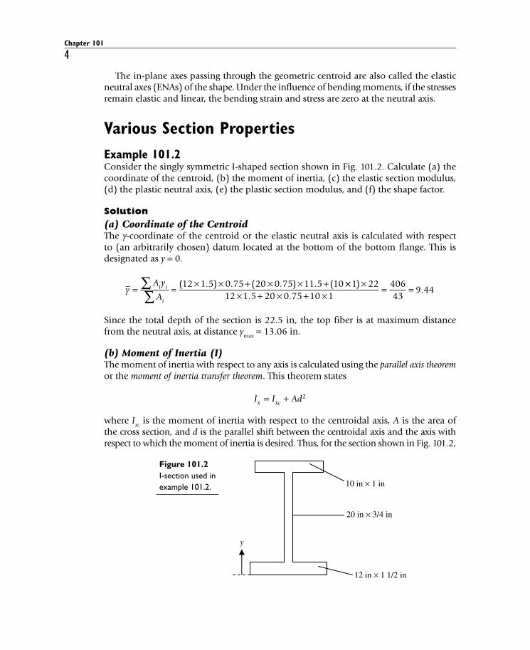
Various Section PropertiesExample 101.2Consider the singly symmetric I-shaped section shown in Fig. 101.2. Calculate (a) the coordinate of the centroid, (b) the moment of inertia, (c) the elastic section modulus, (d) the plastic neutral axis, (e) the plastic section modulus, and (f) the shape factor.
Solution(a) Coordinate of the CentroidThe y-coordinate of the centroid or the elastic neutral axis is calculated with respect to (an arbitrarily chosen) datum located at the bottom of the bottom flange. This is designated as y = 0.
Since the total depth of the section is 22.5 in, the top fiber is at maximum distance from the neutral axis, at distance ymax = 13.06 in.
(b) Moment of Inertia (I)The moment of inertia with respect to any axis is calculated using the parallel axis theorem or the moment of inertia transfer theorem. This theorem states
I I Adx xc= + 2
where Ixc is the moment of inertia with respect to the centroidal axis, A is the area of
the cross section, and d is the parallel shift between the centroidal axis and the axis with respect to which the moment of inertia is desired. Thus, for the section shown in Fig. 101.2,
the moment of inertia about the neutral axis is calculated as the sum of the moments of inertia of the three rectangles—top flange, web, and bottom flange. For each of these rectangles, the local centroidal moment of inertia is given by bh3/12.
INA = × × + × −
+ × ×
112
12 1 5 18 0 75 9 44
112
34
20
3 2
3
. ( . . )
++ × −
+ × × + × − =
15 11 5 9 44
112
10 1 10 22 9 44
2
3 2
( . . )
( . ) 33504 7. in4
NOTE For any shape, the moment of inertia about its centroidal axis has the minimum value. In other words, any other axis parallel to the centroidal axis would produce a greater magnitude of moment of inertia.
(c) Elastic Section Modulus (S)The elastic section modulus of a section is defined as the ratio I/ymax, where ymax rep-resents the distance from the elastic neutral axis to the fiber which is furthest from it. Thus, for the I-section shown in Fig. 101.2, the section modulus is given as
SIcxxc= = =3504 7
13 06268 4
..
. in3
(d) Plastic Neutral Axis (PNA)The plastic neutral axis (PNA) is the line that divides the section into two equal halves. For the section shown, the total area is
A = 18 + 15 + 10 = 43 in2
Therefore, half the area is 21.5 in2.Working upward from the bottom flange, since the area of the bottom flange is 18 in2,
the needed area from the web is 21.5 − 18.0 = 3.5 in2. Therefore, the depth of the web needed is 3.5/0.75 = 4.67 in.
Measured from the bottom, the coordinate of the PNA is yPNA = 1.5 + 4.67 = 6.17 in.
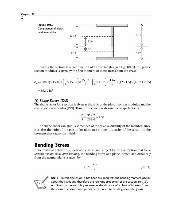
(e) Plastic Section Modulus (Z)The plastic section modulus (Z) is calculated as the sum of the first moments of the two “halves” of the section. Figure 101.3 shows the parts of the I-section with respect to the PNA (y = 6.17). It is convenient to split each T-shaped “half” into its two component rectangles.
Treating the section as a combination of four rectangles (see Fig. 101.3), the plastic section modulus is given by the first moment of these areas about the PNA:
Zx = × × + ×⎛⎝⎜
⎞⎠⎟
× + ×( ) . ..
.10 1 15 8334
15 3315 33
234
4 6674 67
212 1 5 4 67 0 75
352 2
⎛⎝⎜
⎞⎠⎟
× + × × +
=
.( . ) ( . . )
. iin3
(f) Shape Factor (Z/S)The shape factor for a section is given as the ratio of the plastic section modulus and the elastic section modulus (Z/S). Thus, for the section shown, the shape factor is
ZS
= =352 2268 4
1 31..
.
The shape factor can give us some idea of the relative ductility of the member, since it is also the ratio of the plastic (or ultimate) moment capacity of the section to the moment that causes first yield.
Bending StressIf the material behavior is linear and elastic, and subject to the assumption that plane sections remain plane after bending, the bending stress at a plane located at a distance y from the neutral plane, is given by
σb
MyI
= −
(101.3)
NOTE In this discussion, it has been assumed that the bending moment occurs about the x axis and therefore the relevant properties of the section are Ix, Sx, etc. Similarly, the variable y represents the distance of a plane of interest from the x axis. The same concept can be extended to bending about the y axis.
16.33
6.17
15.83
5.42
7.66
2.33
Figure 101.3 Computation of plastic section modulus.
This stress distribution is linear, zero at the neutral plane, and has maximum value at the plane furthest from the neutral plane (y = ymax). Therefore, the maximum bending stress is given by
σmax
max
max
= = =M y
IM
I yMS
x
x
x
x
x
x (101.4)
As the moment is increased, the maximum bending stress reaches the yield stress (Fy).
The moment that causes first yield in the section is given by
M S Fx yyield =
(101.5)
The basis for the following discussion is the elastoplastic model—commonly used for modeling structural steel behavior. In this model, shown in Fig. 101.4, the stress-strain relationship for steel is assumed to be linear and elastic up to the yield point, and then perfectly plastic (E = 0) thereafter. According to this model, the stress remains constant at the yield stress F
y, once the yield strain is exceeded.
Therefore, as the moment is increased beyond Myield, the outer fibers begin to yield and the “plastic behavior zone” gradually progresses inward. The ultimate limit of such a stress distribution is when the plastic zones progress all the way to the neutral axis (all planes at or beyond yield strain). According to the elastoplastic model, there is no more capacity for increased internal stress within the section and therefore, the internal moment capacity is at its maximum. Any increase in load beyond this point will cause the formation of an instability which exhibits itself as a “hinge-like” collapse mechanism. This is referred to as plastic hinge formation. The moment that causes plastic hinge forma-tion is the ultimate moment capacity of the section. This moment can be calculated as
Combined Axial and Bending StressFor a section subject to an eccentric axial load, the total stress is given by
σmax,min = ± = ± = ±
⎡⎣⎢
⎤⎦⎥
PA
MyI
PA
PeyAr
PA
eyr2 21
(101.7)
where r is the radius of gyration of the section.For elements such as prestressed concrete beams, the underlying design philosophy is to avoid (or minimize) tensile stress in the cross section. This may be accomplished by keep-ing the eccentricity of the prestressing force within the “kern” of the cross section. The geo-metric limits of the kern may be calculated by setting the minimum stress equal to zero.
1 02
2
± = ⇒ =eyr
er
ymaxmax
(101.8)
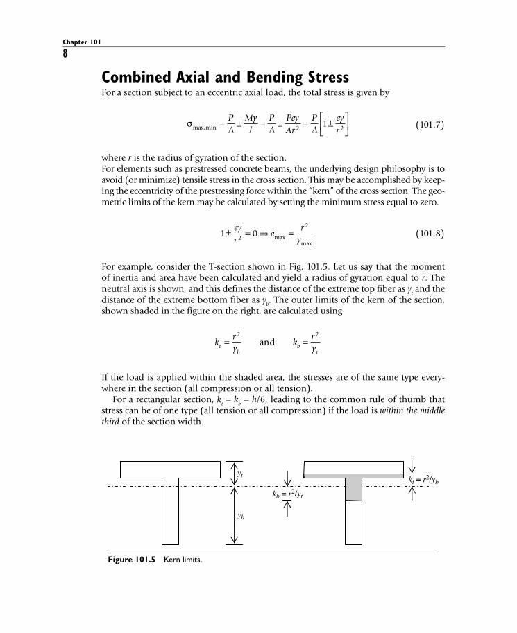
For example, consider the T-section shown in Fig. 101.5. Let us say that the moment of inertia and area have been calculated and yield a radius of gyration equal to r. The neutral axis is shown, and this defines the distance of the extreme top fiber as y
t and the
distance of the extreme bottom fiber as yb. The outer limits of the kern of the section,
shown shaded in the figure on the right, are calculated using
k
ry
kryt
bb
t
= =2 2
and
If the load is applied within the shaded area, the stresses are of the same type every-where in the section (all compression or all tension).
For a rectangular section, kt = k
b = h/6, leading to the common rule of thumb that
stress can be of one type (all tension or all compression) if the load is within the middle third of the section width.
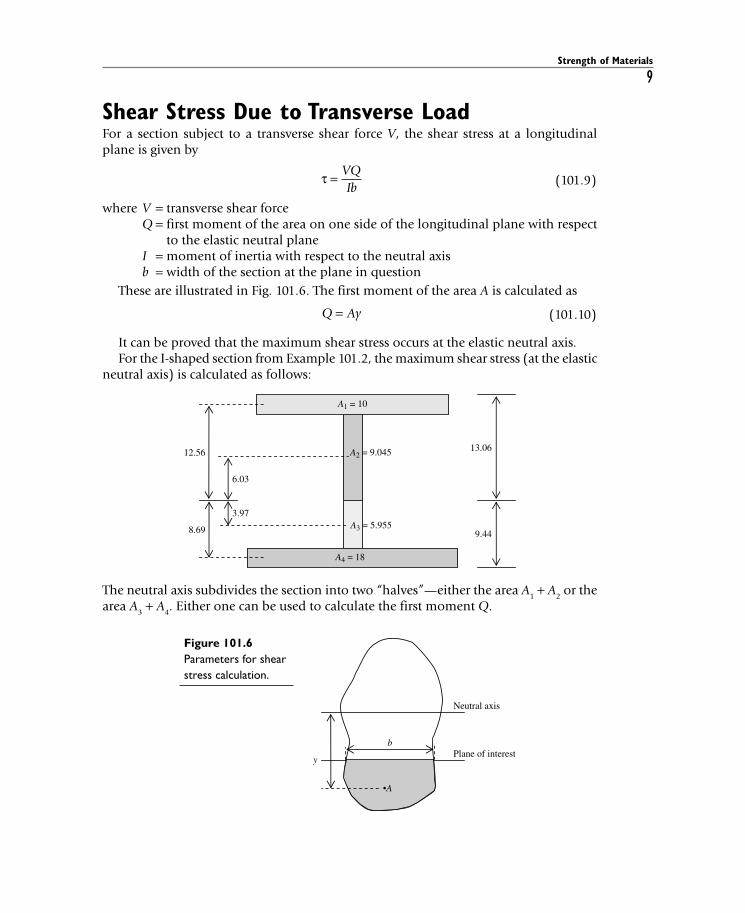
Shear Stress Due to Transverse LoadFor a section subject to a transverse shear force V, the shear stress at a longitudinal plane is given by
τ = VQ
Ib (101.9)
where V = transverse shear force Q = first moment of the area on one side of the longitudinal plane with respect
to the elastic neutral plane I = moment of inertia with respect to the neutral axis b = width of the section at the plane in question
These are illustrated in Fig. 101.6. The first moment of the area A is calculated as
Q Ay= (101.10)
It can be proved that the maximum shear stress occurs at the elastic neutral axis. For the I-shaped section from Example 101.2, the maximum shear stress (at the elastic
neutral axis) is calculated as follows:
13.06
9.44
12.56
8.69
6.03
3.97
A1 = 10
A2 = 9.045
A3 = 5.955
A4 = 18
The neutral axis subdivides the section into two “halves”—either the area A1 + A2 or the area A3 + A4. Either one can be used to calculate the first moment Q.
Neutral axis
Plane of interestb
y
•A
Figure 101.6 Parameters for shear stress calculation.
Using the top half, we have Q = × + × =10 12 56 9 045 6 03 180 1. . . . .in3 Using the bottom half, we have Q = × + × =5 955 3 97 18 8 69 180 1. . . . .in3 If this section is subject to a trans-verse shear stress V = 90 kips, the shear stress can then be calculated as follows. Note that the moment of inertia was previously calculated as I = 3504.7 in4.
τ = = ××
=VQIb
90 180 13504 7 0 75
6 17.
. .. ksi
For I-sections, the flanges play a very small role in resisting shear. Thus, an approximate estimate of the maximum shear stress may be made by distributing the shear force “uniformly” over the web only. In this case, this estimate is given by
τ ≈ =×
=VAw
9020 0 75
6 0.
. ksi
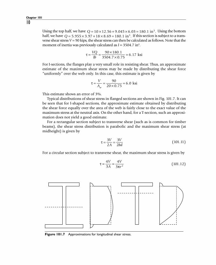
This estimate shows an error of 3%. Typical distributions of shear stress in flanged sections are shown in Fig. 101.7. It can
be seen that for I-shaped sections, the approximate estimate obtained by distributing the shear force equally over the area of the web is fairly close to the exact value of the maximum stress at the neutral axis. On the other hand, for a T-section, such an approxi-mation does not yield a good estimate.
For a rectangular section subject to transverse shear (such as is common for timber beams), the shear stress distribution is parabolic and the maximum shear stress (at midheight) is given by
τ = =3
232
VA
Vbd
(101.11)
For a circular section subject to transverse shear, the maximum shear stress is given by
τ
π= =4
34
3 2
VA
Vr
(101.12)
Figure 101.7 Approximations for longitudinal shear stress.
Shear Stress Due to Torsion—Circular SectionsWhen a solid circular section (radius R) is subjected to torsion, the shear stress between adjacent planes is given by
τ = Tr
J (101.13)
where J is the polar moment of inertia of the section, given by
J
R= π 4
2 (101.14)
Thus, the maximum shear stress in a solid circular shaft due to a torque T is given by
τ
π πmax /= =TR
RTR4 32
2
(101.15)
For a hollow cylindrical shaft (inner radius R1 and outer radius R2), the polar moment of inertia is given by
J
R R=
−π( )24
14
2 (101.16)
and the maximum shear stress is given by
τ
πmax ( )=
−2 2
24
14
TRR R
(101.17)
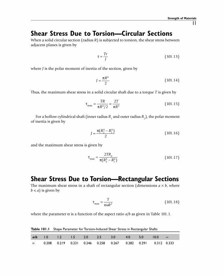
Shear Stress Due to Torsion—Rectangular SectionsThe maximum shear stress in a shaft of rectangular section (dimensions a × b, where b < a) is given by
τ
αmax = Tab2
(101.18)
where the parameter α is a function of the aspect ratio a/b as given in Table 101.1.
Shear Stress Due to Torsion—Thin-Walled SectionsEconomy of weight leads to hollow thin-walled sections being commonly used for structural members subject to significant torsional moments. The thin-walled assump-tion is considered approximately valid when the wall thickness is less than about 1/20 of the lateral dimension. The maximum shear stress in a thin-walled hollow shaft is given by
τmax = T
A tm2 (101.19)
where T = applied torque A
m = area enclosed by the closed wall centerline of the section (see Fig. 101.8)
t = thickness of the thinnest part of the wall
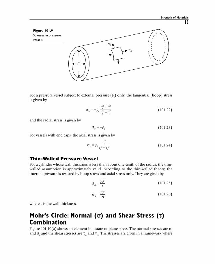
Stresses in Pressure VesselsA cylindrical pressure vessel is shown in Fig. 101.9. The inner radius is r
i and the outer
radius is ro.
For a pressure vessel subject to internal pressure (pi) only, the tangential (hoop)
For a pressure vessel subject to external pressure (po) only, the tangential (hoop) stress
is given by
σh o
o i
o i
pr rr r
= −+−
2 2
2 2
(101.22)
and the radial stress is given by
σr op= −
(101.23)
For vessels with end caps, the axial stress is given by
σa i
i
o i
pr
r r=
−
2
2 2
(101.24)
Thin-Walled Pressure VesselFor a cylinder whose wall thickness is less than about one-tenth of the radius, the thin-walled assumption is approximately valid. According to the thin-walled theory, the internal pressure is resisted by hoop stress and axial stress only. They are given by
σh
ip rt
=
(101.25)
σa
ip rt
=2
(101.26)
where t is the wall thickness.
Mohr’s Circle: Normal (σ) and Shear Stress (τ) CombinationFigure 101.10(a) shows an element in a state of plane stress. The normal stresses are σ
the axes are the “traditional” x-y axes—a horizontal x axis and a vertical y axis. Some-times, the engineer might be more interested in stresses oriented along a different set of axes. A “rotated” element (rotated counterclockwise through angle θ) is shown in Fig. 101.10(b). This element has “new” stress components—σ
x’ and σy’, τx’y’ and τ
y’x’.This “new” stress-state is not independent of the original stress-state, but rather a
function of it (transformed). The transformation relations are given by Eqs. (101.27).
σσ σ σ σ
θ τ θ
σσ σ σ
′
′
=+
+−
+
=+
−
xx y x y
xy
yx y
2 22 2
2
cos sin
xx yxy
x yx y
xy
−−
= −−
+′ ′
σθ τ θ
τσ σ
θ τ
22 2
22
cos sin
sin coos 2θ
(101.27)
A very convenient way of (graphically) expressing these results is through Mohr’s circle. By eliminating θ from Eqs. (101.27), we can write
σσ σ
τσ σ
′ ′ ′−+⎛
⎝⎜
⎞
⎠⎟ + −( ) =
−⎛
⎝⎜
⎞
⎠⎟ +x
x yx y
x y
20
2
22
2
ττxy2
(101.28)
σy
σxσx
τxy
τxy
τyx
τyx
σy ′
σy ′
σx′
σx′
τy ′x′
τy ′x′
τx′y′
τx′y′
θ
θ
(a) (b)
Figure 101.10 Stresses on 2D element (a) original (b) transformed.
This represents the equation of a circle with center at
σ σx y+⎛
⎝⎜
⎞
⎠⎟2
0,
and radius
R x yxy=
−⎛
⎝⎜
⎞
⎠⎟ +
σ στ
2
2
2
See Fig. 101.11. Each point on Mohr’s circle represents the stress-state along a particular plane. Maximum and minimum normal stresses are designated σmax and σmin respectively.
These are also called the principal stresses. Note that these principal directions have only normal stress, i.e., the principal directions are free of shear stress.
σ σ σσ σ σ σ
τmax min, = ± =+
±−⎛
⎝⎜
⎞
⎠⎟ +ave R x y x y
xy2 2
2
2
(101.29)
The maximum and minimum values of σx’ are calculated by setting d dxσ θ′ =/ 0 . These
normal stresses (principal stresses) occur at two specific values of θ, given by
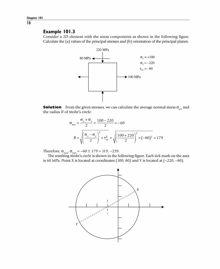
Example 101.3Consider a 2D element with the stress components as shown in the following figure. Calculate the (a) values of the principal stresses and (b) orientation of the principal planes.
100 MPa
220 MPa
80 MPa σx = +100
σy = –220
τxy = –80
Solution From the given stresses, we can calculate the average normal stress σave and the radius R of Mohr’s circle:
σσ σ
σ στ
ave =+
= − = −
=−⎛
⎝⎜
⎞
⎠⎟ +
x y
x yxyR
2100 220
260
2
2
22
2
2100 2202
80 179= +⎛⎝⎜
⎞⎠⎟
+ − =( )
Therefore, σmax, σmin = −60 ± 179 = 119, −239. The resulting Mohr’s circle is shown in the following figure. Each tick mark on the axes
is 60 MPa. Point X is located at coordinates (100, 80) and Y is located at (−220, −80).
The values of maximum and minimum normal stress can also be calculated by taking the derivative of σ
x’ with respect to θ.
σσ σ σ σ
θ τ θ
σθ
σ
′
′
=+
+−
+
= − −
xx y x y
xy
xx
dd
2 22 2cos sin
( σσ θ τ θ
θτ
σ σ
y xy
xy
x y
)sin cos
tan( )
2 2 2 0
22 2 8
+ =
=−
= × − 00100 220
160320
0 5+
= − = − .
This yields 2θ = tan−1 (−0.5) = −26.6° or 153.4°.Substituting 2θ = −26.6°, we get σ
x’ = −60 + 160 × 0.894 + 80 × 0.447 = 119. Substitut-ing 2θ = 153.4°, we get σ
x’ = −60 − 160 × 0.894 − 80 × 0.447 = −239. Note that the point with normal stress σ = 119 is located at a position which is 26.6° clockwise (thus nega-tive) with respect to the point X and σ = −239 is located at a position which is 153.4° counterclockwise (thus positive) with respect to X.
Indeterminate Problems in Strength of MaterialsA (statically) indeterminate problem is one for which equations of static equilibrium are necessary but not sufficient for a complete solution. In such cases, compatibility equations must be used in addition to equilibrium equations.
Example 101.4A composite short column has a steel core (diameter 10 in) surrounded by a snug brass sleeve (inner diameter 10 in, outer diameter 12 in). The column is loaded uniformly (using loading plates) in compression. If the compressive load is 200 kips, what is the stress in the steel? Assume Esteel = 29000 ksi and Ebrass = 17000 ksi.
Solution The only equilibrium equation available is
Psteel + Pbrass = 200 kips
This is not enough to solve for the two unknowns, Psteel and Pbrass. The additional equa-tion is the compatibility equation that states
Δsteel = Δbrass
Asteel = π ⁄4 (10)2 = 78.54 in2
Abrass = π ⁄4 (122 − 102) = 34.56 in2
P LA E
P LA E
PA EA E
PS
S S
B
B BS
S S
B BB= ⇒ = = ×78 54
34 5629.
.0000
170003 877× =P PB B.
Thus,
4.877 Pbrass = 200 k ⇒ Pbrass = 41 k and Psteel = 159 k
Stress in the steel (assuming uniform distribution of load):
σsteel = 159/78.54 = 2.02 ksi
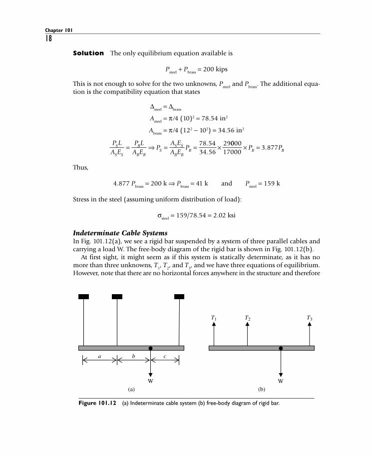
Indeterminate Cable SystemsIn Fig. 101.12(a), we see a rigid bar suspended by a system of three parallel cables and carrying a load W. The free-body diagram of the rigid bar is shown in Fig. 101.12(b).
At first sight, it might seem as if this system is statically determinate, as it has no more than three unknowns, T1, T2, and T3, and we have three equations of equilibrium. However, note that there are no horizontal forces anywhere in the structure and therefore
W
T1 T2 T3
a b c
W(a) (b)
Figure 101.12 (a) Indeterminate cable system (b) free-body diagram of rigid bar.
applying the ΣFx = 0 equation would simply result in a trivial equation of the form 0 = 0.
Thus, we have only two useful equations at our disposal: ΣFy = 0 and ΣM
z = 0. Therefore,
the system is first-order indeterminate (two equations, three unknowns).The two equations of static equilibrium are
F T T T W
M T a W a b T a b
y = ⇒ + + − =
= ⋅ − ⋅ + + ⋅ +
∑∑
0 01 2 3
1 2 3( ) ( ++ =c) 0
The third equation is implicit in a single word in the statement of the problem—”rigid” bar. If the bar is (for all practical purposes), infinitely more rigid than the rest of the components of the system, then we can assume that, as the force W pulls down on the assembly, the cables stretch and the bar moves downward, but in such a way that the bar remains straight (no bending deformation). As a result, the deflected shape of the assembly will look somewhat as shown in Fig. 101.13.
Applying similar triangles, as shown in Fig. 101.14
Δ Δ Δ Δ
Δ Δ Δ Δ
Δ
2 1 3 2
3 2 2 1
1
−=
−+
− = + −
+
a b c
a b c
b c
( ) ( )( )
( ) −− + + + =( )a b c aΔ Δ2 3 0
a
Δ1 Δ2Δ3
b + cFigure 101.13 Deflection of rigid bar.
a b + c
Δ2 – Δ1
Δ3 – Δ2
Δ3Δ2Δ1Figure 101.14 Compatibility of deflections using similar triangles.
This is our missing third equation. The three equations can now be solved simultane-ously to calculate T1, T2, and T3.
Example 101.5 A rigid bar ABC is suspended by three cables as shown. Data for the three cables are given in the table following. All cables are steel (E = 29000 ksi).
Cable Length (ft) Diameter (in)
1 4.0 0.25
2 3.0 0.40
3 5.0 0.30
12
3
2 ft
20 k
x
6 ft
AB
C
Find the distance (x) at which the 20-kip load must be applied such that the bar ABC remains horizontal.