Chapter Two

Fourier Series

1. Introduction. All of the eigenfunctions found in the last chapter for the eigenvalue

problem

φ′′(x) = µφ(x)

subject to the various boundary conditions were combinations of sines and cosines and thus

periodic functions. We recall that a function f defined on (−∞,∞) is periodic with period

p if

f(x+ p) = f(x) for all x ∈ (−∞,∞).

Since f(x +mp) = f(x + (m − 1)p) = · · · = f(p) it follows that any periodic function with

period p also has period mp for any integer m. For example, the functions sin(mωx) and

cos(mωx) have period p = 2π/mω since

sin(mω(x+ p)) = sin(mωx+ 2π).

Note that this identity implies that 2π/ω is the period common for all these functions for

m = 1, 2, . . . .

It now follows that the orthogonal projection Pf of a square integrable function f defined

on [0, L] into the span of trigonometric functions is automatically defined on (−∞,∞), and

if all of these functions have a common period p then Pf is periodic on the whole line with

period p. Let us look at the eigenfunction expansions discussed in Chapter ST. If

MN = span{sinλnx}, λn = nπ/L, n = 1, 2, . . .

then Pf has period 2L. Moreover, since each sine function is odd it follows that Pf is an

odd 2L periodic function on (−∞,∞). If

MN = span{sinλnx}, λn =(π

2+ nπ

)/L, n = 0, 1, 2, . . .

then Pf is an odd periodic function with period 4L. Moreover, it follows from the addition

formula

sin(x+ y) = sin x cos y + cos x sin y

that

sin

(π2

+ nπ)(L + ∆L)

L= sin

(π2

+ nπ)(L− ∆L)

Lfor ∆L > 0

1

so that this 4L periodic function is also even with respect to x = L. Similarly, if

MN = span{cosλnx}, λn =(π

2+ nπ

)/L, n = 0, 1,

then Pf is an even approximation of f defined on (−∞,∞) with period 4L. Moreover, the

addition formula

cos(x+ y) = cos x cos y − sin x sin y

shows that

Pf(L+ ∆L) = −Pf(L− ∆L)

so that Pf also is odd with respect to x = L.

However, the orthogonal projection Pf into the span of eigenfunctions associated with

boundary conditions like

u(0) = 0, u′(L) = u(L)

is not periodic on (−∞,∞) because in general sin λmx and sinλnx have no common period.

Let us now turn to the eigenfunctions{cos mπx

L, sin nπx

L

}associated with

φ′′(x) = µφ(x)

φ(0) = φ(L)

φ′(0) = φ′(L).

The Sturm-Liouville theory assures that the orthogonal projection Pf of a function f in

L2[0, L] converges in the mean square sense to f . However, for these functions a great

deal more is known about their approximating properties than just mean square conver-

gence. These periodic functions are the basis of Fourier series approximations to continuous

and discontinuous periodic functions which are widely used in signal recognition and data

compression and, of course in diffusion and vibration studies. We shall give next a fairly

self-contained outline of the mathematics of Fourier series.

Let X be the linear space of all continuous, piecewise smooth functions that are periodic

with period 2L for some L > 0 with the usual definitions of addition and scalar multiplica-

tion. (The function f is piecewise continuous if it has at most a finite number of jump

discontinuities on any finite interval. It is piecewise smooth if it is piecewise continuous

2

and on every finite interval has a piecewise continuous derivative except at possible a finite

number of points.) It is easy to verify that with inner product

(f, g) =

L∫

−L

f(x)g(x)dx,

the sequence

{1, cos

πx

L. sin

πx

L, cos 2

πx

L, sin 2

πx

L, cos 3

πx

L, sin 3

πx

L, . . .

}

is an orthogonal sequence. It is clear that the inner product (1, 1) = 2L and also easy to

verify that

(sinn

πx

L, sinn

πx

L

)=

L∫

−L

sin2 nπt

Ldt = L, and

(cos n

πx

L, cosn

πx

L

)=

L∫

−L

cos2 nπt

Ldt = L.

Thus for an integer N , the best least squares approximation Sn(x) of f ∈ X by a linear

combination of

{1, cos

πx

L. sin

πx

L, cos 2

πx

L, sin 2

πx

L, cos 3

πx

L, sin 3

πx

L, . . . , cosN

πx

L, sinN

πx

L

}

is given by

Sn(x) =a0

2+

N∑

n=1

(an cosn

πx

L+ bn sinn

πx

L

),

where

an =1

L

L∫

−L

f(t) cosnπt

Ldt, and bn =

1

L

L∫

−L

f(t) sinnπt

Ldt.

The seriesa0

2+

∞∑

n=1

(an cosn

πx

L+ bn sinn

πx

L

)

is called the Fourier series of f , named for the French mathematician Joseph Fourier

(1768-1830), who introduced it in his solutions of the heat equation−more of this later. The

fact that a series is the Fourier series of a function f is usually indicated by the notation

f ∼

a0

2+

∞∑

n=1

(an cosn

πx

L+ bn sinn

πx

L

).

The coefficients an and bn are called the Fourier coefficients of f .

3

Proposition 2.1. Suppose an and bn are the Fourier coefficients of f . Then the series∞∑

j=1

(a2k + b2k) converges.

Proof : Applying Bessell’s inequality to the orthonormal sequence

{1√2L,

1√L

cosπx

L,

1√L

sinπx

L,

1√L

cos 2πx

L,

1√L

sin 2πx

L,

1√L

cos 3πx

L,

1√L

sin 3πx

L, . . .

}

gives us

a20L

2+ L

∞∑

n=1

(a2n + b2n) ≤

2L∫

0

(f(x))2dx,

from which the proposition follows at once. The next proposition is an easy consequence

of Riemann’s Lemma.

Proposition 2.2. limn→∞

L∫−L

f(t) cosnπtLdt = lim

n→∞

L∫−L

f(t) sinnπtLdt = 0.

Is the given orthogonal sequence is an approximating basis? That is a good question

which we shall address in this chapter. We shall also investigate not only mean convergence

of this series in several different subspaces of X, but also other types of convergence.

2. Convergence. Before we come to grips with convergence questions regarding the

Fourier series, a brief review of the convergence of sequences of functions is in order. We

shall look at three different types of convergence. Let us recall the definitions.

Definition. A sequence (fn) of functions all with domain D is said to converge point-

wise to the function f if for each x ∈ D it is true that fn(x) → f(x).

Definition. A sequence (fn) of functions all with domain D is said to converge uni-

formly to the function f if given an ε > 0, there is an integer N so that |fn(x) − f(x)| < ε

for all n ≥ N and all x ∈ D.

Definition. A sequence (fn) of functions all with domain D = [a, b] is said to converge

in the mean to the function f ifb∫

a

[fn(x) − f(x)]2 dx→ 0.

A few examples will help illuminate these definitions. For each positive integer n ≥ 2

and for x ∈ [0, 1], let

fn(x) =

n2x if 0 ≤ x ≤ 1/n−n2(x− 1

n) + n if 1/n < x ≤ 2/n

0 if 2/n < x ≤ 1.

Thus, fn looks like

4

(1/n,n)

2/n

It should be clear that for each x ∈ [0, 1], we have limn→∞

fn(x) = 0. Thus the sequence

(fn) converges pointwise to the function f(x) = 0. Note that this sequence does not, however,

converge uniformly to f(x) = 0. In fact, for every n, there is an x ∈ [0, 1] such that

|fn(x) − f(x)| ≥ n.

Next, note that1∫

0

(fn(x))2 dx =2

3n,

which tells us that (fn) does not converge in the mean to f .

Next, for each integer n ≥ 1 and x ∈ [0, 1], let

fn(x) =

{n− n3x if 0 ≤ x ≤ 1/n3

0 if 1/n3 < x ≤ 1.

A picture:

1/n^3

n

5

It is clear that1∫0

(fn(x))2dx = 13n

, and so our sequence converges in the mean to f(x) = 0.

Clearly it does not converge pointwise or uniformly.

We see next that uniform convergence is the nicest of the three.

Theorem 2.3. Suppose the sequence (fn) of functions with domain [a, b] converges

uniformly to the function f . Then (fn) converges pointwise to f and also converges in the

mean to f .

Proof : It is obvious that the sequence converges to f pointwise. For convergence in the

mean, let ε > 0 and choose n sufficiently large to insure that |fn(x) − f(x)| <√ε/(b− a)

for all x ∈ [a, b]. Then

b∫

a

|fn(x) − f(x)|2 dx <b∫

a

ε

b− adx = ε.

Hence, (fn) converges in the mean to f .

We shall make use of the so-called Weierstrass M-test, named for the German

mathematician Karl Weierstrass (1815-1897), given in the following theorem.

Theorem 2.4. Consider the series of functions∞∑

n=0

gn(x) for x ∈ [a, b]. If for all n,

we have |gn(x)| ≤ Mn for all x ∈ [a, b] and if∞∑

n=0

Mn converges, then∞∑

n=0

gn(x) converges

uniformly and absolutely on [a, b].

Proof : First, we show absolute convergence. Let ε > 0. Choose N so thatn∑

k=m

Mk <

ε for n,m > N. Then for n,m > N,

n∑

k=m

|gk(x)| ≤n∑

k=m

Mk.

Thus∞∑

n=0

|gn(x)| converges to a limit function G(x).

Now, to see the convergence to G(x) is uniform, let ε > 0 and choose N so thatn∑

k=m

Mk < ε/2 for all n ≥ N .

∣∣∣∣∣

n∑

k=0

gk(x) −G(x)

∣∣∣∣∣ ≤∣∣∣∣∣

m∑

k=0

gk(x) −G(x)

∣∣∣∣∣ +

∣∣∣∣∣

n∑

k=m

gk(x)

∣∣∣∣∣

≤∣∣∣∣∣

m∑

k=0

gk(x) −G(x)

∣∣∣∣∣ +n∑

k=m

Mk

6

3. Uniform convergence of Fourier series. Suppose f is a piecewise smooth con-

tinuous function of period 2L. We shall show that the Fourier series

f ∼

a0

2+

∞∑

n=1

(an cosn

πx

L+ bn sinn

πx

L

),

converges uniformly to some function g. Notice that this will not establish that the orthog-

onal sequence

{1, cos

πx

L. sin

πx

L, cos 2

πx

L, sin 2

πx

L, cos 3

πx

L, sin 3

πx

L, . . .

}

in the space of continuous piecewise smooth functions with the usual inner product is an

approximating basis because it does not say that the function g is the function f with which

we started. This is in fact the case, but a proof of must wait until later.

Theorem 2.5. If f is a piecewise smooth continuous function, the Fourier series of f

converges uniformly.

Proof : Let g(x) = f ′(x) at all points where f has a derivative. Define g(x) = 0 at

the other points—recall there are only a finite number of them on any any bounded interval.

Let

an =1

L

L∫

−L

f(t) cosnπt

Ldt, bn =

1

L

L∫

−L

f(t) sinnπt

Ldt,

An =1

L

L∫

−L

g(t) cosnπt

Ldt, and Bn =

1

L

L∫

−L

g(t) sinnπt

Ldt

be the Fourier coefficients of f and g. Integration by parts tells us that for n ≥ 1,

An = nbn and Bn − nan.

Hence,n∑

j=1

(a2j + b2j)

1/2 =

n∑

j=1

1

j(A2

j +B2j )

1/2.

From the Cauchy-Schwartz inequality, we see that

n∑

j=1

(a2j + b2j)

1/2 =n∑

j=1

1

j(A2

j +B2j )

1/2 ≤[

n∑

j=1

1

j2

]1/2 [n∑

j=1

(A2j +B2

j )

]1/2

.

7

We know∞∑

j=1

1j2 converges and Proposition 1 tells us that

∞∑j=1

(A2j + B2

j ) converges. Hence

∞∑j=1

(a2j + b2j)

1/2 converges also. Observing that a cos θ+ b sin θ = (a2n + b2n)1/2 sin(θ+ϕ), where

tanϕ = a/b, we see that∣∣∣an cosn

πx

L+ bn sin n

πx

L

∣∣∣ ≤ (a2n + b2n)1/2

The Weierstrass M-test now tells us that the Fourier series

a0

2+

∞∑

n=1

(an cosn

πx

L+ bn sinn

πx

L

)

converges uniformly and absolutely.

It is worth repeating what this theorem does not say. It does not tell us that the

uniform limit of the series is the function f .

4. Pointwise convergence of Fourier series. A few preliminary results are in order

first.

Proposition 2.6. If θ is not an integral multiple of 2π, then

1

2+

n∑

k=1

cos kθ =sin(n + 1

2)θ

2 sin(θ/2).

Proof : Let

S =1

2+

n∑

k=1

cos kθ.

Then

2S sinθ

2= sin

θ

2+

n∑

k=1

2 cos kθ sinθ

2.

We remember that

2 cosα sin β = sin(α + β) − sin(α− β)

so the above equation becomes

2S sinθ

2= sin

θ

2+

n∑

k=1

[sin(k +

1

2)θ − sin(k − 1

2)θ

]

= sinθ

2+

n∑

k=1

sin(k +1

2)θ −

n∑

k=1

sin(k − 1

2)θ

= sinθ

2+

n∑

k=1

sin(k +1

2)θ −

n−1∑

k=0

sin(k +1

2)θ

= sin(n+1

2)θ.

8

Hence,

S =sin(n+ 1

2)θ

2 sin θ2

.

Proposition 2.7. If k is an integer, then limθ→2kπ

sin(n+ 1

2)θ

2 sin θ

2

= n+ 12.

Definition. The function

Dn(θ) =1

2+

n∑

k=1

cos kθ =

{sin(n+ 1

2)θ

2 sin θ

2

if θ 6= 2kπ

n+ 12

if θ = 2kπ

is continuous and periodic with period 2π. (This function is called the Dirichlet kernel,

named for the German mathematician Lejeune Dirichlet (1805-1859). )

Integrate the formula in Proposition 2.6 to get

Proposition 2.8.2π∫0

Dn(θ)dθ = π.

Notation. The left and right hand limits of f at x are denoted by f(x−) and f(x+),

respectively. In other words

f(x−) = limh→0

f(x− h), and f(x+) = limh→0

f(x + h), where h > 0.

Theorem 2.9. Let f be a piecewise smooth function of period 2π. The the Fourier series

of f converges pointwise to the function

f̃(x) =f(x+) + f(x−)

2.

Proof : Let

f ∼

a0

2+

∞∑

n=1

(an cosnx + bn sinnx) .

Note that because f is piecewise smooth f and f̃ differ at at most a finite number of points

on any bounded interval. Thus the Fourier series for f and f̃ are the same.

Now then,

an cos nx+ bn sin nx =1

π

2π∫

0

f̃(t) [cosnt cosnx + sinnt sin nx] dt

=1

π

2π∫

0

f̃(t) cosn(x− t)dt.

Hence,

Sn(x) =a0

2+

N∑

n=1

(an cos nx+ bn sin nx) =1

π

2π∫

0

f̃(t)

[1

2+

N∑

n=0

cosn(x− t)

]dt,

9

and so from Proposition 2.6, we have

SN(x) =a0

2+

N∑

n=1

(an cosnx + bn sinnx) =1

π

2π∫

0

f̃(t)sin(N + 1

2)(x− t)

2 sin((x− t)/2)dt,

or,

SN(x) =1

π

2π∫

0

f̃(t)DN(x− t)dt =1

π

2π∫

0

f̃(x− t)DN (t)dt.

We also have

SN(x) = − 1

π

−2π∫

0

f̃(x + t)DN(−t)dt =1

π

2π∫

0

f̃(x + t)DN(t)dt.

(Remember that the Dirichlet kernel is an even function and DN and f̃ both have period

2π.)

Next from Proposition 2.8,

SN(x) − f̃(x) = SN(x) − f̃(x)1

π

2π∫

0

DN(t)dt

=1

π

2π∫

0

[f̃(x− t) − f̃(x)

]DN (t)dt,

and

SN(x) − f̃(x) =1

π

2π∫

0

[f̃(x + t) − f̃(x)

]DN(t)dt.

Adding these two, we have

2[SN(x) − f̃(x)] =1

π

2π∫

0

[f̃(x− t) + f̃(x+ t) − 2f̃(x)]DN(t)dt.

Next observe that the integrand in this expression is an even function. Thus,

SN(x) − f̃(x) =1

π

π∫

0

[f̃(x− t) + f̃(x+ t) − 2f̃(x)]DN(t)dt

Next, note that 2f̃(x) = f(x+) + f(x−), and so we have

SN(x) − f̃(x) =1

π

π∫

0

[f̃(x− t) + f̃(x + t) − f(x+) − f(x−)]DN (t)dt

=1

π

π∫

0

[f̃(x− t) − f(x−)]DN (t)dt+1

π

π∫

0

[f̃(x+ t) − f(x+)]DN (t)dt.

10

We shall show that

limN→∞

(SN(x) − f̃(x)

)= 0

by showing that

limN→∞

π∫

0

[f̃(x− t) − f(x−)]DN (t)dt = limN→∞

π∫

0

[f̃(x+ t) − f(x+)]DN(t)dt = 0.

First, look at [f̃(x− t) − f(x−)]DN (t).Observe that the function F defined by

F (t) =f̃(x− t) − f(x−)

t

t

2 sin t/2

is perfectly nice at t = 0:

limt→0+

f̃(x− t) − f(x−)

t= f ′(x−) and lim

t→0+

t

2 sin t/2= 1.

Thus,

F̃ (t) =

{f̃(x−t)−f(x−)

tt

2 sin t/20 < t ≤ π

f ′(x−) t = 0

is piecewise smooth on [0, π].

Now,

[f̃(x− t) − f(x−)]DN (t) =f̃(x− t) − f(x−)

t

t

2 sin t/2sin(N +

1

2)t

= F̃ (t) cos t/2 sinNt + F̃ (t) sin t/2 cosNt.

Hence,

π∫

0

[f̃(x− t) − f(x−)]DN (t)dt =

π∫

0

F̃ (t) cos t/2 sinNtdt +

π∫

0

F̃ (t) sin t/2 cosNtdt.

Finally, observe that

{sin t, sin 2t, sin 3t, . . .} and {cos t, cos 2t, cos 3t, . . .}

are orthogonal sequences with the inner product (u, v) =π∫0

u(t)v(t)dt.The Riemann lemma

then tells us that

limN→∞

π∫

0

F̃ (t) cos t/2 sinNtdt = limN→∞

π∫

0

F̃ (t) sin t/2 cosNtdt = 0.

11

Thus we have finally shown that

limN→∞

π∫

0

[f̃(x−t)−f(x−)]DN (t)dt = limN→∞

π∫

0

F̃ (t) cos t/2 sinNtdt+ limN→∞

π∫

0

F̃ (t) sin t/2 cosNtdt = 0

The demonstration that

limN→∞

π∫

0

[f̃(x+ t) − f(x+)]DN(t)dt = 0

is almost the same and is omitted. This at last proves the theorem.

This result allows use to tidy up the loose ends of Theorem 2.5. Recall that this one

told us that the Fourier series of a continuous piecewise differentiable function f converges

uniformly to something but did not say what. Now we know from the just proved Theorem

2.9 that the something to which the series converges must indeed be f . This is worth stating

explicitly.

Corollary 2.10. If f is continuous, then the series converges uniformly to f .

Remark. Although the theorem refers to functions having period 2π, it applies as well

to other periodic functions; the choice of 2π is simply a computational convenience. Given

a function f having period 2L, apply Theorem 2.9 to the function F (x) = f(xL/π).

Example. Let us find the Fourier series for the function f(x) = x on the interval [−π, π] :

ak =1

π

π∫

−π

f(t) cos ktdt =1

π

π∫

−π

t cos ktdt = 0,

bk =1

π

π∫

−π

f(t) sin ktdt =1

π

π∫

−π

t sin ktdt =1

k2(sin kt− kt cos kt)

∣∣∣∣π

−π

= −2

kcos kπ = (−1)k+1 2

k

The Fourier series is thus

2

∞∑

k=1

(−1)k+1

ksin kx

Now, what does the limit of this series look like? We simply apply Theorem 2.9 to

the periodic extension of f . This results in

12

–3

–2

–1

1

2

3

–5 5 10x

Another example. We shall find the Fourier series of the function g(x) = |x| on the

interval [−1, 1].

a0 =

1∫

−1

|t| dt = 1

an =

1∫

−1

|t| cosnπtdt = 2

1∫

0

t cos nπtdt = 2−1 + (−1)n

n2π2for n ≥ 1;

bn =

1∫

−1

|t| sinnπtdt = 0.

Life can be made a bit simpler by noting that for n ≥ 1

an =

{0 if n even−4

n2π2 if n odd.

Then letting n = 2k + 1, we have the Fourier series

1

2− 4

π2

∞∑

k=0

1

(2k + 1)2cos(2k + 1)πx.

Now, where does this series converge and what does the limit look like? Again, we

simply look at the periodic extension of f . A picture:

0

0.2

0.4

0.6

0.8

1

–4 –2 2 4x

13

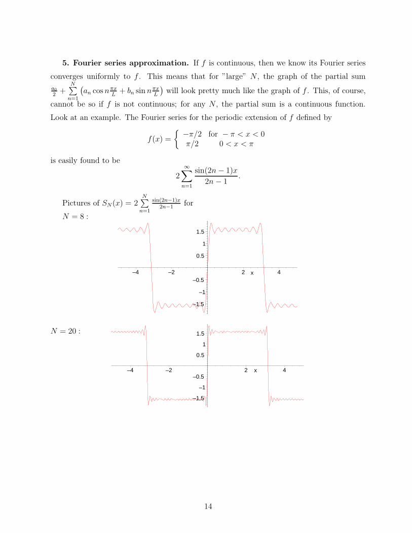
5. Fourier series approximation. If f is continuous, then we know its Fourier series

converges uniformly to f . This means that for ”large” N , the graph of the partial sum

a0

2+

N∑n=1

(an cosnπx

L+ bn sin nπx

L

)will look pretty much like the graph of f . This, of course,

cannot be so if f is not continuous; for any N , the partial sum is a continuous function.

Look at an example. The Fourier series for the periodic extension of f defined by

f(x) =

{−π/2 for − π < x < 0π/2 0 < x < π

is easily found to be

2∞∑

n=1

sin(2n− 1)x

2n− 1.

Pictures of SN (x) = 2N∑

n=1

sin(2n−1)x2n−1

for

N = 8 :

–1.5

–1

–0.5

0.5

1

1.5

–4 –2 2 4x

N = 20 :

–1.5

–1

–0.5

0.5

1

1.5

–4 –2 2 4x

14

N = 30 :

–1.5

–1

–0.5

0.5

1

1.5

–4 –2 2 4x

One might hope that the limiting graph is simply the graph of f with vertical lines

at the points of discontinuity. It is, as the pictures seem to indicate, not to be so. It turns

out that we inevitably have a situation like that indicated in the examples of Section 2 in

which the sequence of functions SN(x) converges pointwise to the limit f , but no matter

how large N is, there will be values of x at which the difference |SN(x) − f(x)| is larger than

some fixed value. Let us see precisely what we are talking about. First with this specific

example, and then in general.

Proposition 2.11. Let

g(x) =

{−π/2 for − π < x < 0π/2 0 < x < π

,

and let

Sn(x) = 2

n∑

k=1

sin(2k − 1)x

2k − 1

be the nth partial sum of the Fourier series for g.Then for given ε > 0, there is an integer N

such that ∣∣∣∣∣∣Sn(

π

2n) −

π∫

0

sin t

tdt

∣∣∣∣∣∣< ε for all n > N.

Proof : First, observe that

d

dxSn(x) = 2

n∑

k=1

cos(2k − 1)x =sin 2nx

sin x

Thus,

Sn(x) =

x∫

0

sin 2nt

sin tdt, and so

Sn(x) −x∫

0

sin 2nt

tdt =

x∫

0

sin 2nt

[1

sin t− 1

t

]dt

15

Now, note that

limt→0

[1

sin t− 1

t

]= 0

and so there is a number K so that∣∣sin 2nt

[1

sin t− 1

t

]∣∣ ≤ K for all t ∈ [−π, π]. Thus

∣∣∣∣∣∣Sn(x) −

x∫

0

sin 2nt

tdt

∣∣∣∣∣∣=

∣∣∣∣∣∣

x∫

0

sin 2nt

[1

sin t− 1

t

]dt

∣∣∣∣∣∣≤ Kx

Let ε > 0 be given and choose δ so that∣∣∣∣∣∣Sn(x) −

x∫

0

sin 2nt

tdt

∣∣∣∣∣∣< ε for 0 < x < δ.

Next, observe thatx∫

0

sin 2nt

tdt =

2nx∫

0

sin t

tdt

so that we have ∣∣∣∣∣∣Sn(x) −

2nx∫

0

sin t

tdt

∣∣∣∣∣∣< ε for 0 < x < δ.

Choose N large enough to ensure that π/2N < δ. Then for n > N , letting x = π/2n, we

have ∣∣∣∣∣∣Sn(x) −

2nx∫

0

sin t

tdt

∣∣∣∣∣∣=

∣∣∣∣∣∣Sn(

π

2n) −

π∫

0

sin t

tdt

∣∣∣∣∣∣< ε,

and the proposition is proved.

Comment. Note that∞∫0

sin ttdt = π/2. Thus Sn( π

2n) −

π∫0

sin ttdt = Sn(

π2n

) − π2

+∞∫π

sin ttdt.

Hence,

limn→∞

[Sn(

π

2n) − π

2

]= lim

n→∞

[Sn(

π

2n) − g(

π

2n)]

= −∞∫

π

sin t

tdt ≈ 0.281 14.

You can see this in the graphs pictured above.

Let us reflect on what all this tells us. We know that for fixed x 6= 0 in the interval

(−π, π), the sequence (sn(x)) converges to π/2. Thus we can have Sn(x) as close to π/2 ≈1. 570 8 as we wish by choosing n large enough. There is, on the other hand, an x (viz.,

x = π/2n) such that Sn(x) is as close toπ∫0

sin ttdt ≈ 1. 851 9 as we wish. As we shall see

in the sequel, this behavior is not restricted just to this particular function, but is seen at

16

any point at which the piecewise smooth function f fails to be continuous. This behavior is

called the Gibbs Phenomenon, in honor of the American physicist, J. Willard Gibbs

(1839-1903).

Now we seen about the general case.

Theorem 2.12. Suppose f is piecewise smooth and continuous everywhere on the

interval [−π, π] except at x = 0.Let fn(x) be the nth partial sum of the Fourier series for f .

Then

limn→∞

[fn(

π

2n) − f(

π

2n)]

= [f(0+) − f(0−)]−1

π

∞∫

π

sin t

tdt

Proof : Let ψ(x) = f(x) − 12[f(0+) + f(0−)] − 1

π[f(0+) − f(0−)] g(x), where g is

the function defined in Proposition 2.11.Then

ψ(0+) = f(0+) − 1

2[f(0+) + f(0−)] − 1

π[f(0+) − f(0−)]

π

2= 0, and

ψ(0−) = f(0−) − 1

2[f(0+) + f(0−)] +

1

π[f(0+) − f(0−)]

π

2= 0.

Thus ψ is continuous at 0 and hence everywhere on the given interval. In particular, the

sequence (ψn(x)) of partial sums of its Fourier series converges uniformly to ψ.Hence,

limn→∞

[ψn(

π

2n) − ψ(

π

2n)]

= 0.

Now

ψn(π

2n) − ψ(

π

2n) = fn(

π

2n) − f(

π

2n) − 1

π[f(0+) − f(0−)]

(gn(

π

2n) − π

2

);

and so

limn→∞

{fn(

π

2n) − f(

π

2n) − 1

π[f(0+) − f(0−)]

(gn(

π

2n) − π

2

)}= 0.

Thus,

limn→∞

[fn(

π

2n) − f(

π

2n)]

= limn→∞

1

π[f(0+) − f(0−)]

(gn(

π

2n) − π

2

)

= [f(0+) − f(0−)]−1

π

∞∫

π

sin t

tdt

Comment. The theorem shows that the Gibbs Phenomenon ”overshoot” at the jump

discontinuity is −1π

∞∫π

sin ttdt ≈ 8. 949 0× 10−2 times the total jump of f .

17

6. Cosine and sine series. In our discussion of orthogonal collections of eigenfunctions,

we also considered the approximation of functions by a series of cosine functions and sine

functions. We shall now look at these in more detail. Mercifully, most of the results are easy

consequence of what we have done for the Fourier series.

Let X be the linear space of all continuous, piecewise smooth functions that are

periodic with period L for some L > 0. Then we know the collection

{1, cos

πx

L. cos 2

πx

L, cos 3

πx

L, . . .

}

is an approximating base that is orthogonal with respect to the inner product (f, g) =L∫0

f(t)g(t)dt. For f ε X, we thus have mean convergence to f of the series

A0

2+

∞∑

n=1

An cosnπx

L, where

An =(f, cos nπx

L)

(cosnπxL, cosnπx

L)

=2

L

L∫

0

f(t) cosnπt

Ldt.

Now, let f̃ be defined by

f̃(x) =

{f(−x) for − L < x < 0f(x) for 0 ≤ x < L

.

Observe that f̃ is an even function.

Now, compute the Fourier series for f̃ (more precisely. for the periodic extension of

f̃ .):

an =1

L

L∫

−L

f̃(t) cosnπt

Ldt = an =

2

L

L∫

0

f(t) cosnπt

Ldt = An,

since the integrand is an even function. And

bn =1

L

L∫

−L

f̃(t) sin nπt

Ldt = 0,

since the integrand is an odd function. In other words, the above series

A0

2+

∞∑

n=1

An cosnπx

L

18

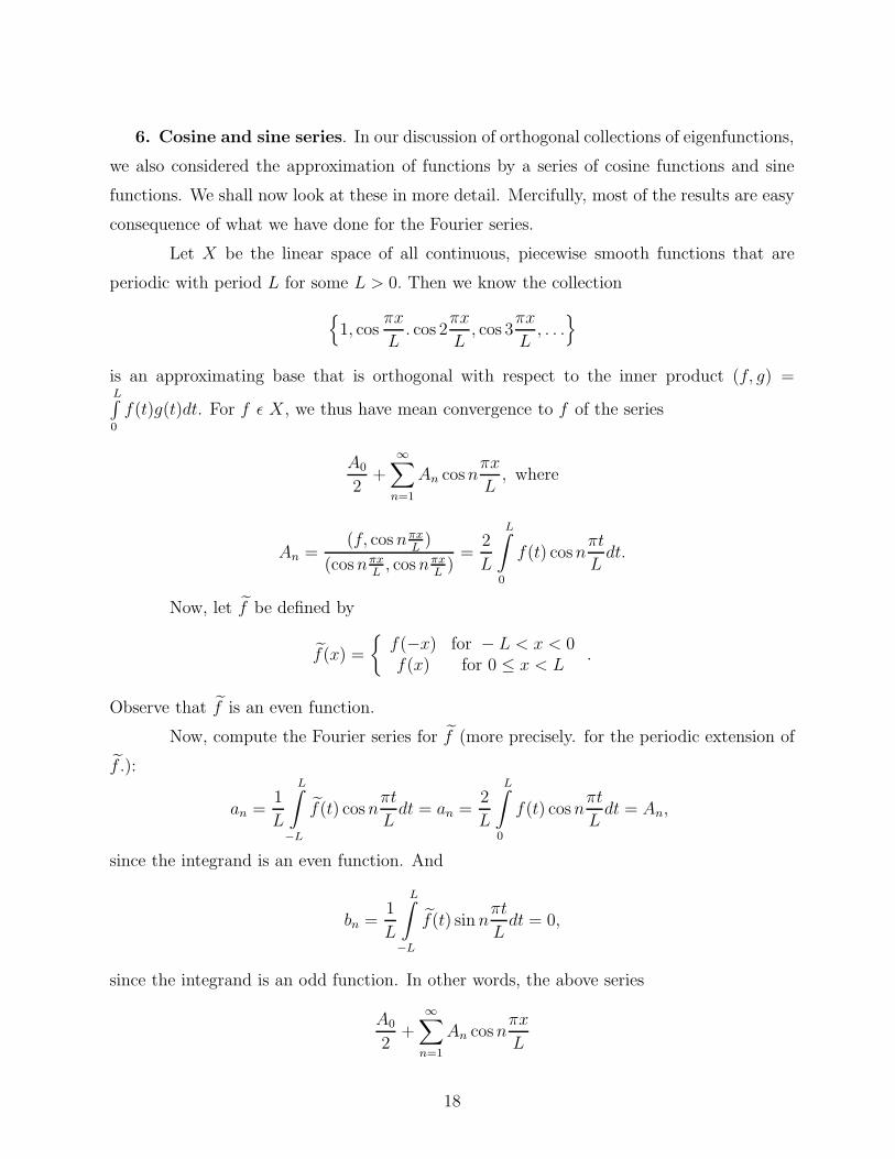
is “really” the Fourier series for the extension f̃ . This means we know all about it! The series

is usually called the Fourier cosine series for f .

Example. Let f be defined by f(x) = x for 0 ≤ x ≤ π. Then f̃ , the even extension of

f looks like

The cosine series is

c(x) =π

2+

2

π

∞∑

k=1

(−1)k − 1

k2cos kx;

and it converges to this:

The collection {sin

πx

L, sin 2

πx

L, sin 3

πx

L, . . .

}

is also an orthogonal approximating basis for the space X. It is easy to show that the

Fourier sine series for a function f

∞∑

n=1

Bn sinnπx

L,

19

where

Bn =2

L

L∫

0

f(t) sinnπt

Ldt

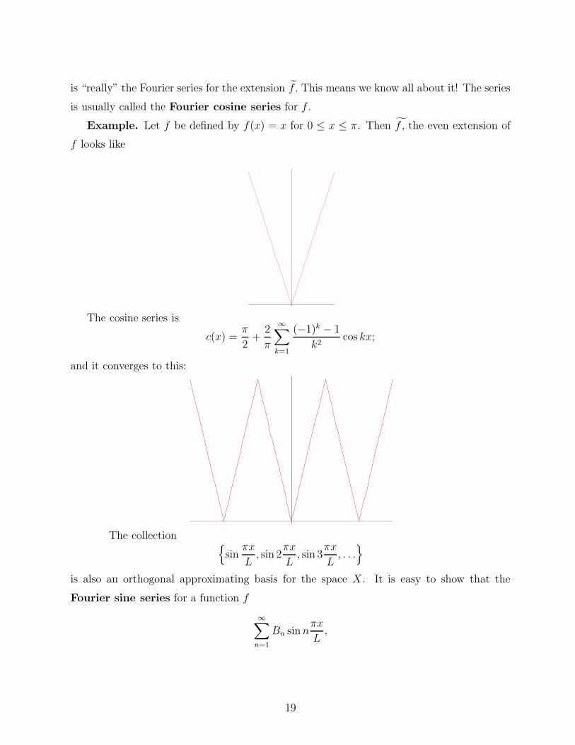
is the Fourier series of the odd periodic extension f̂ of f :

f̂(x) =

{−f(−x) −L < x < 0f(x) 0 ≤ x < L

.

Example. Let f be as in the previous example. Then f̂ looks like

–3

–2

–1

0

1

2

3

–3 –2 –1 1 2 3x

Here is the sine series:

s(x) = 2∞∑

k=1

(−1)k+1

ksin kx.

The limit of this series is thus

–3

–2

–1

1

2

3

–8 –6 –4 –2 2 4 6 8x

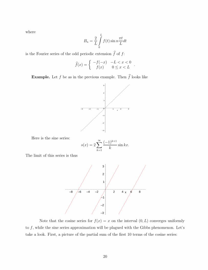
Note that the cosine series for f(x) = x on the interval (0, L) converges uniformly

to f , while the sine series approximation will be plagued with the Gibbs phenomenon. Let’s

take a look. First, a picture of the partial sum of the first 10 terms of the cosine series:

20

0.5

1

1.5

2

2.5

3

0 0.5 1 1.5 2 2.5 3x

0

0.5

1

1.5

2

2.5

3

0.5 1 1.5 2 2.5 3x

Although on the interval (0, π) both the cosine and the sine series converge pointwise

to f(x) = x, the convergence of the sine series is much nastier because the odd extension of

f is not continuous.

21