CHAPTER VI Beyond Light: Physical, Geological and Chemical ...

Light availability has been identified as the majorfactor controlling the distribution and abundance

of SAV in Chesapeake Bay (e.g., Dennison et al. 1993).Therefore, parameters that can affect the light avail-ability in an environment (total suspended solids,chlorophyll a concentration, epiphyte biomass) arecommonly included in predictions of the suitability ofcertain areas for SAV growth. Several other parame-ters that have the potential to override the lightrequirements of the plants are not often consideredwhen determining the suitability of a site for SAVgrowth (Livingston et al. 1998). For example, very highwave energy may prevent SAV from becoming estab-lished (due to the drag exerted on the plants and/orthe constant sediment motion), even when the lightrequirements are met (Clarke 1987).

This chapter discusses physical, geological and chemi-cal factors that affect the suitability of a site for SAVgrowth. These factors differ from those described inchapters III, IV and V in that the parameters consid-ered there modify the light requirements of SAV. Theparameters discussed in the present chapter overridethe established SAV light requirements. The parame-ters addressed here (waves, currents, tides, sedimentorganic content, grain size and contaminants) caninfluence the presence/absence of SAV in a certainarea, independently of light levels. Figure VI-1 showshow previously established SAV habitat requirements(light attenuation coefficient, dissolved inorganicnutrients, chlorophyll a, total suspended solids andepiphytes) as well as the parameters discussed in thischapter (waves, currents, tides, sediment characteris-

tics and chemical contaminants) can affect the distri-bution of SAV.

FEEDBACK BETWEEN SAV AND THE PHYSICAL, GEOLOGICAL AND CHEMICALENVIRONMENTS

SAV beds can reduce current velocity (Fonseca et al.1982; Fonseca and Fisher 1986; Gambi et al. 1990;Koch and Gust 1999; Sand-Jensen and Mebus 1996;Rybicki et al. 1997), attenuate waves (Fonseca andCahalan 1992; Koch 1996), change the sediment char-acteristics (Scoffin 1970; Wanless 1981; Almasi et al.1987; Wigand et al. 1997) and even change the heightof the water column (Powell and Schaffner 1991;Rybicki et al. 1997). In turn, these SAV-inducedchanges can affect the productivity of the plants.Therefore, a complex feedback mechanism existsbetween SAV and the abiotic conditions of the habitatthey colonize, making it difficult to attribute the distri-bution of SAV to only one factor, such as light.

By reducing current velocity and attenuating waves,SAV beds create conditions that lead to the depositionof small (inorganic) and low-density (organic) parti-cles within meadows or canopies (Grady 1981; Kempet al. 1984; Newell et al. 1986). This in turn can affectthe availability of light (Moore et al. 1994), nutrients(Kenworthy et al. 1982) and compounds that can betoxic to SAV (phytotoxins), such as sulfide in the sedi-ments (Carlson et al. 1994; Holmer and Nielsen 1997).Therefore, all these parameters contribute, to somedegree, to the regulation of SAV growth.

Chapter VI – Beyond Light: Physical, Geological and Chemical Habitat Requirements 71

CHAPTER VVII

Beyond Light: Physical, Geologicaland Chemical Habitat Requirements

72 SAV TECHNICAL SYNTHESIS II

Light Transmission

Waves Tides

PlanktonChlorophyll a

Total SuspendedSolids

DIN

DIP Epiphytes

Grazers

Organic matter Sulfide

N

P

Contaminants

Biogeo-chemicalprocesses

Settlingof

OrganicMatter

SAV

PLL

PLW

Currents

FIGURE VI-1. Interaction between Light-Based, Physical, Geological and Chemical SAV HabitatRequirements. Interaction between previously established SAV habitat requirements, suchas light attenuation, dissolved inorganic nitrogen (DIN), dissolved inorganic phosphorus(DIP), chlorophyll a, total suspended solids (TSS) and other physical/chemical parametersdiscussed in this chapter (waves, currents, tides, sediment organic matter, biogeochemicalprocesses). P = phosphorus; N = nitrogen; PLW = percent light through water; PLL =percent light at the leaf.

When plant density is low, the attenuation of currentvelocity and wave energy is also low. This results in lit-tle accumulation of organic matter and, subsequently,little change in sediment nutrient and phytotoxin con-centrations. Light availability may also be low, due tothe resuspension of sediments. Oxygen demand of theroots (to counteract the detrimental effect of the phy-totoxins) may also be low, due to reduced photosyn-thetic biomass.

In SAV beds with high shoot density, water flow isreduced and more particles are deposited, leading tohigher light, nutrient and phytotoxin availability thanin less dense beds. The SAV density may reach a pointwhere so much organic matter is trapped that theresulting high phytotoxin levels are no longer toleratedby the plants, and they may start dying back (Roblee etal. 1991; Carlson et al. 1994; Holmer and Nielsen1997). At that point, the reduction in density may leadto higher water flow, reduced organic matter ac-cumulation and reduced phytotoxin levels in the sedi-ment. This feedback mechanism (hydrodynamics ➝sediment characteristics ➝ plant biomass ➝ hydrody-namics) may assure the health of marine and highersalinity estuarine SAV populations over time. Theabove mechanism may be less applicable for SAV col-onizing low-salinity estuarine areas, because sulfideconcentrations do not reach levels as toxic as those inmarine environments. However, low-salinity speciescan also be susceptible to sulfide, as shown by thedecreased growth rates of Potamogeton pectinatuswhen sulfide was added to the sediments (van Wijk et al. 1992).

SAV AND CURRENT VELOCITY

SAV beds reduce current velocity by extractingmomentum from the moving water (Madsen andWarnke 1983). The magnitude of this process dependson the density of the SAV bed (Carter et al. 1991; vanKeulen 1997), the hydrodynamic conditions of thearea (stronger reduction in flow in tide-dominated vs.wave-dominated areas; Koch and Gust 1999) and thedepth of the water column above the plants (Fonsecaand Fisher 1986). The highest reduction in currentvelocity occurs in dense, shallow beds exposed to tide-dominated conditions (unidirectional flow). Currentsin SAV beds can be 2 to 10 times slower than in adja-cent unvegetated areas (Ackerman 1983; Madsen and

Warncke 1983; Carter et al. 1988; Gambi et al. 1990;Rybicki et al. 1997).

Positive Effects of Reduced Current Velocity

The advantages of reduced water flow in SAV bedsinclude the following:

1) Reduced self-shading due to the more verticalposition of the blades in beds resulting fromreduced drag on SAV leaves (Fonseca et al. 1982);

2) Increased settlement of organic and inorganic par-ticles, increasing the light availability and the sedi-ment nutrient concentration (Kenworthy et al.1982; Ward et al. 1984; references in the review byFonseca 1996). Notice that this can also lead to adisadvantage due to increasing sulfide concentra-tion in marine/higher salinity estuarine habitats(Koch 1999) (see “Negative Effects of ReducedCurrent Velocity”).

3) Lower friction velocities at the sediment surfacethan in unvegetated areas (Fonseca and Fisher1986) reducing sediment resuspension and totalsuspended solids concentrations and increasinglight availability (references in the review byFonseca 1996).

4) High residence time, allowing molecules of dis-solved nutrients to stay in contact with SAV leavesand epiphytes for longer periods of time, thereforeincreasing the likelihood of being taken up. As aresult, high residence time reduces the nutrientconcentration in the water column (Bulthuis et al.1984), perhaps limiting epiphytic growth, whichwould otherwise lead to further reduction in lightattenuation (see Chapter V). Epiphytes and SAVwill compete for nutrients in the water column,while only SAV can remove nutrients from the sed-iments. Therefore, the SAV should not become asnutrient-limited as epiphytes since they primarilyuse nutrients from the sediments.

5) Increased settlement of spores of algae and larvaeof a variety of organisms, resulting in higherspecies diversity of invertebrates and algae in SAVcanopies than in adjacent unvegetated areas(Homziak et al. 1982).


Negative Effects of Reduced Current Velocity

The points listed above illustrate the potential positiveeffects of reduced current velocity in SAV beds. Alter-nately, reduced water flow can also have detrimentaleffects:

1) Concentration of phytotoxins will increase in estu-arine/marine sediments (Koch 1999). The concen-tration of phytotoxins in the sediment leads to anincreased oxygen demand by the roots which, if notmet due to poor light availability, has the potentialto kill the plants (Robblee et al. 1991; Carlson et al.1994; Nepf and Koch 1999).

2) Thicker blade diffusion boundary layers will formunder reduced current velocity in SAV beds (Koch1994). The diffusion boundary layer is a thin (a fewµm) layer of water on the surface of any submersedobject (including plants) where the transport ofsolutes (e.g. carbon needed for photosynthesis oroxygen produced by photosynthesis) is dominatedby viscous forces (i.e., by diffusion).

Increases in the thickness of this diffusion boundarylayer lead to a longer diffusional path (or thick diffu-sion boundary layer) for carbon molecules to movefrom the water column to the SAV leaf, where they areused for photosynthesis. As the current velocitydecreases, a critical maximum diffusion boundarylayer thickness, where the flux of carbon to the plant isslower than the flux needed for the plant to supportmaximum photosynthesis, can be reached. The criticaldiffusion boundary layer thickness was estimated to be280 µm for Thalassia testudinum and 98 µm forCymodocea nodosa (Koch 1994).

If a plant is exposed for long periods of time to diffu-sion boundary layer thicknesses greater than the criti-cal diffusion boundary layer thickness, growth candecline, due to carbon limitation independent of thelight levels at the site. The length of time that a plantcan survive under such conditions depends on theinternal carbon reserves in the plant tissue and howfast these reserves can be accessed (Koch 1993). Thishas not yet been determined for most SAV species andhas the potential to be important in areas where mari-nas and other structures may cause stagnant condi-tions in SAV habitats.

Some estuarine and freshwater SAV species, such asPotamogeton pectinatus, are capable of colonizing rela-tively stagnant waters (like those found in ponds) due

to a physiological adaptation: the release of H+ on oneside of the blade (polar leaves) reduces the pH in thediffusion boundary layer (Prins et al. 1982). Thisdecrease in pH shifts the carbon balance toward car-bon dioxide (CO2), increasing local diffusion boundarylayer CO2 concentration and, therefore, increasing theflux of CO2 into the plant. Other SAV can also incor-porate CO2 from sediment porewater, where dissolvedinorganic carbon concentrations are usually muchhigher than open-water concentrations (Sondergaardand Sand-Jensen 1979; Madsen 1987). The CO2 incor-porated by the roots is then transported to the photo-synthetic tissue via the lacunae system (Madsen andSand-Jensen 1991). For a detailed discussion on mech-anisms aquatic plants developed to deal with reducedcarbon fluxes due to thick diffusion boundary layers,see Jumars et al. (accepted).

Epiphytes and Current Velocity

Although epiphytes are usually seen as organisms thatare detrimental to SAV growth, the very early stages ofepiphytic colonization on SAV leaves have the poten-tial to be beneficial for the plants (Koch 1994). Verylow densities of epiphytes (only visible under a micro-scope) may disrupt the diffusion boundary layerenhancing the flux of carbon to the blade (Koch 1994).As epiphytes compete for light, nutrients and carbon,later stages of epiphytic colonization (when the epi-phytic layer is too dense to disrupt the diffusionboundary layer) become detrimental to SAV growth.At the community level, epiphytes will contribute tothe reduction in current velocity (due to increased leafdrag) which leads to the positive aspects listed above(see “Positive Effects of Reduced Current Velocity”).Therefore, in some aspects, epiphytes can have posi-tive effects on SAV communities, although the nega-tive effects of epiphytes on SAV leaves (lightattenuation and increased drag on the leaves, poten-tially dislodging them at high flows) also need to bekept in perspective.

Epiphytes on SAV leaves may also respond to waterflow independently of the SAV response to flow. In astudy using acrylic plates, maximum periphyton bio-mass was observed at intermediate current velocities.Diatoms were dominant under high current conditionswhile a green alga was dominant at lower currentvelocities (Horner et al. 1990). In a mesocosm experi-ment, epiphyte biomass on Vallisneria americana


increased with current velocity (Merrell 1996). There-fore, a second order of complexity (water flow) needsbe added to future refinements of the model evaluat-ing the effect of epiphytes on light available to SAVleaves (see Chapter V).

Current Velocity SAV Habitat Requirements

From the positive and negative effects of the reducedcurrent velocities found in SAV beds, it can be con-cluded that these plants could benefit from intermedi-ate current velocities (Boeger 1992; Koch and Gust1999; Merrell 1996; Koch 1999). Extremely low waterflows could increase the blade diffusion boundarylayer thickness as well as the accumulation of organicmatter in the sediment leading to carbon starvation ordeath due to high phytotoxin concentrations in thesediment, respectively. In contrast, extremely highwater flow has the potential to 1) increase drag abovea critical value where erosion of the sediment andplants occurs, 2) reduce light availability throughresuspension of sediment and self-shading and 3)decrease the accumulation of organic matter, leadingto reduced nutrient concentration in the sediments.

A literature review revealed that 1) the range of cur-rent velocities tolerated by marine SAV species liesbetween approximately 5 and 100 cm s-1 (physiologicaland mechanical limits, respectively); 2) the range ofcurrent velocities tolerated by freshwater SAV speciesseems generally to be lower than that for the marinespecies; and 3) some freshwater SAV species can tol-erate extremely low current velocities (Table VI-1).This may be due to alternative mechanisms of carbonacquisition present in these freshwater plants but notin marine plants (see “Negative Effects of ReducedCurrent Velocity”).

Survival of SAV in high current velocity environmentsmay be possible if the development of seedlingsoccurred under conditions of slow current velocity inspace (e.g., a protected cove) or time (e.g., a low waterdischarge period). Once a bed is established undersuch conditions, it can expand into adjacent areas withhigher currents due to the reduced currents at theedge of the bed or persist during times of higher waterflow. Therefore, the stage of the plants (for example,seeds, seedlings, vegetative shoots, reproductiveshoots) also needs to be taken into account when con-sidering if current velocity is above or below the estab-lished requirement for growth and distribution. Based

on the literature review presented here, no data areavailable on the current velocity requirements ofplants other than those found in well-established beds.

In summary, intermediate current velocities between10 and 100 cm s-1 are needed to support the growthand distribution of healthy marine SAV beds. Theserequirements are lower for freshwater/estuarine SAVspecies—between 1 and 50 cm s-1—especially for thosewith polar leaves. If currents are above or below thesecritical levels, the feedback mechanisms in the systemmay become imbalanced and possibly lead to thedecline or even complete loss of the vegetation.Although some of the feedback mechanisms betweenSAV beds and current velocity involve light availabilitythrough the effects of resuspension of sediments, self-shading and epiphytic growth, extreme currents alonecan limit the growth of SAV. Therefore, currentvelocity should be considered as a key SAV habitatrequirement.

SAV AND WAVES

As waves propagate over SAV beds, wave energy is lost(Fonseca and Cahalan 1992; Koch 1996). This is due tothe same mechanism that causes SAV beds to reducecurrent velocities–loss of momentum (Kobayashi et al.1993). The efficiency with which waves are attenuatedby SAV beds depends on the water depth (Ward et al.1984; Mork 1996), the current velocity (Stewart et al.1997), leaf length (Fonseca and Cahalan 1992) and thetype of vegetation (canopy or meadow) (Elwany et al.1995; Mork 1996; Stewart et al. 1997).

Wave attenuation is strongest in dense SAV beds dueto increased drag and in meadows (where most of thebiomass is found close to the sediment surface) colo-nizing shallow waters, where plant biomass takes up alarge portion of the water column. Canopy-formingspecies that have long stems and concentrate most oftheir biomass, and consequently drag, on the watersurface of a relatively deep water body have the ten-dency to oscillate with the waves. Acting as thoughimbedded in the waves, canopy-forming speciesimpose little drag on them (Seymour 1996) and, there-fore, have little effect on wave attenuation.

The effect the constant motion waves imposes onplants may lead to the breakage of the plants(Idestam-Almquist and Kautsky 1995; Stewart et al.



TABLE VI-1. Minimum and maximum current velocities required for SAV growth and distribution.

1997). This effect has been observed to be more severefor a canopy-forming species (Myriophyllum spp.) thanfor a meadow-forming species (Vallisneria spp.; Stew-art et al. 1997). Breakage of underwater plants exposedto waves is inversely related to current velocity. As cur-rent velocity increases, the plants lie closer to the sed-iment surface and are, therefore, less affected by theorbital motion of the waves (Stewart et al. 1997).

Table VI-2 summarizes the capacity of marine SAVspecies to attenuate waves under a variety of field andlaboratory conditions. The values obtained in the labare much higher than those obtained in the field,because the meadow-forming plants used in the labexperiments occupied the entire water column, and wave attenuation is positively correlated with thepercentage of the water column occupied by thevegetation.

Effects of High Wave Energy

The impact of high wave energy on SAV can be director indirect. The direct impact of waves on SAV can beseen when waves (in combination with currents) erodethe edges of an SAV bed (Clarke 1987) or when por-tions of the plants are removed by storm-generated(Thomas et al. 1961; Eleuterius and Miller 1976;Rodriguez et al. 1994; Dan et al. 1998) or boat-generated waves (Stewart et al. 1997). Indirect conse-quences of wave energy in SAV beds include sedimentresuspension, changes in sediment grain size, mixingof the water column and epiphytic growth. If thecapacity of an SAV bed to attenuate waves is reduced,for example, due to a reduction in shoot densitybecause of clam dredging or eutrophication, theunderlying sediment will become more vulnerable toerosion, and higher concentrations of suspended


TABLE VI-2. Attenuation of wave energy in meadow-forming marine SAV beds.

sediment particles can be expected in the water. Thisis especially true for SAV beds in which fine particleshave accumulated over time. These sediments may beresuspended at lower wave energy than the coarsersediments outside the SAV bed (Posey et al. 1993).

Wave attenuation and sediment resuspension in vege-tated areas depend on the water levels above theplants. At low tide, wave energy is reduced to a greaterextent than during high tide (Ward et al. 1984). Resus-pension of fine particles will alter the grain size distri-bution of the sediment. In areas of high waveexposure, sediments are coarser, which leads to lowernutrient concentration in the sediment and, conse-quently, lower root biomass (Idestam-Almquist andKautsky 1995). By contrast, the above-ground biomassof Potamogeton pectinatus depends directly on waveexposure; shoots are shorter in areas with high waveexposure than in areas with low wave exposure(Idestam-Almquist and Kautsky 1995).

In Chesapeake Bay, shore erosion (caused by waveaction) contributes 13 percent of the total suspendedmatter in the upper Bay and 52 percent in the middleBay (Biggs 1970). Perhaps, before the decline of SAVin this area, SAV protected the coastlines from the

direct impact of waves. Ward et al. (1984) observedthat in shallow (< 2 meters) unvegetated areas in theChoptank River, total suspended solids concentrationsincreased tenfold when the wind came from the direc-tion of highest fetch and was >25 km h-1, but theincreased total suspended solids concentrations dissi-pated within 24 hours after the storm. As the windintensifies, wave period and wave length increase lead-ing to deeper wave mixing depths (Chambers 1987).The small grain size sediments are the first to becomeresuspended. Therefore, if wave energy increases in anSAV bed, a shift toward coarser sediments will occur.The consequences of this shift are addressed below, in“SAV and the Sediments It Colonizes.”

SAV growth and distribution seems to be limited byhigh, but not low wave energy (Dan et al. 1998; TableVI-3). However, high wave exposure can also benefitthe plants by reducing the epiphytic biomass (Strandand Weisner 1996; Kendrick and Burt 1997; Weisner etal. 1997). In high wave exposure areas, where sedi-ments are constantly being shifted and grain size maybe skewed toward coarser particles, SAV may not beable to become established due to the balance betweenthe anchoring capacity of the roots and the dragexerted on the leaves. High wave exposure also leads


TABLE VI-3. Quantitative and qualitative descriptions of wave tolerance for Chesapeake Bay species.

to reduced light availability due to increased sedimentresuspension, but this may be compensated by thelower epiphytic biomass on the leaves of wave-exposedplants. The mechanism that allows for reduced epi-phytic biomass on plants exposed to high wave energyis not well understood. It could be due to the rubbingof the blades against each other.

Wave Mixing Depth Effects on SAV Minimum Depth Distributions

The minimum depth of distribution of aquatic plantsin lakes with good water quality has been correlated tothe resuspension of sediments by waves resulting inthe scouring of sediments, uprooting of plants andincreased turbidity (Figure VI-2). Consequently,Chambers (1987) suggested that the minimum depthdistribution (Zmin) of aquatic plants can be determinedby the wave mixing depth (Zwave), which extends to adepth equal to half the wavelength (L),

Zmin = Zwave = L (VI-1).2

L can be calculated from the wave period (T) using thefollowing equation:

(VI-2)

where g is acceleration of gravity (9.805 m s-2). Equa-tion VI-2 is a standard equation for waves propagatingover depths larger than half the wavelength (i.e.,before they “feel the bottom” and define Zmin; seeEquation VI-1). The wave period (T) for these wavescan be predicted according to the following equation:

(VI-3)

where W is the wind velocity (m s-1) and F is the effec-tive fetch (m). These equations allow for the predic-tion of the wave mixing depth (Zwave) in shallow SAV habitats.

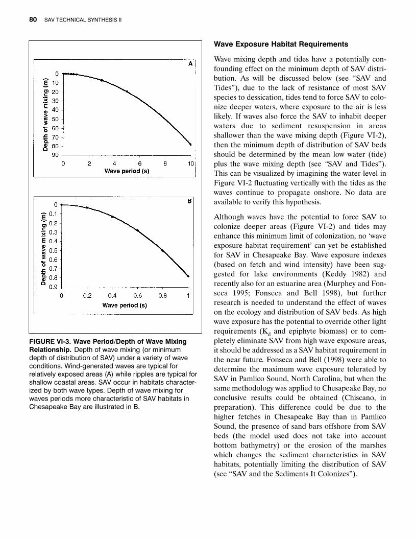
In relatively exposed areas at the mouth of Chesa-peake Bay (Timble Shoal Entrance and Timble ShoalLight), wave periods (T) range between 4 and 13 sec-onds (Boon et al. 1996). These values are typical forwind- generated waves. Marine SAV can colonize suchareas, as seen in the Thalassia testudinum beds off-shore of the Florida Keys (Koch 1996), the Cymodoceanodosa beds in the Mediterranean (Koch 1994) andthe Posidonia oceanica beds in many areas in Aus-tralia. In the shallower, more protected SAV habitatsin Chesapeake Bay, waves with smaller periods(ripples) can be expected. Figure VI-3a shows thewave mixing depth for ripples and wind-generatedwaves while Figure VI-3b shows more details for rip-ples, typical for shallow, semi-enclosed SAV habitats.

]WgF][

g0.46W[=T 0.28

2

p2gT=L

2


FIGURE VI-2. Wave Energy Effects on SAV Vertical Depth Distributions. The vertical distribution of SAV beds can be shifted into deeper waters due to wave energy. Waves can constantly shift sediments preventing the colonization of the area or resuspend sediments, contributing to increased total suspended solid (TSS) concentrations, which leads to reduced light levels. The zone where waves do not allow SAV to colonize is defined as the depth equivalent to half the wavelength.

Wave Exposure Habitat Requirements

Wave mixing depth and tides have a potentially con-founding effect on the minimum depth of SAV distri-bution. As will be discussed below (see “SAV andTides”), due to the lack of resistance of most SAVspecies to dessication, tides tend to force SAV to colo-nize deeper waters, where exposure to the air is lesslikely. If waves also force the SAV to inhabit deeperwaters due to sediment resuspension in areasshallower than the wave mixing depth (Figure VI-2),then the minimum depth of distribution of SAV bedsshould be determined by the mean low water (tide)plus the wave mixing depth (see “SAV and Tides”).This can be visualized by imagining the water level inFigure VI-2 fluctuating vertically with the tides as thewaves continue to propagate onshore. No data areavailable to verify this hypothesis.

Although waves have the potential to force SAV tocolonize deeper areas (Figure VI-2) and tides mayenhance this minimum limit of colonization, no ‘waveexposure habitat requirement’ can yet be establishedfor SAV in Chesapeake Bay. Wave exposure indexes(based on fetch and wind intensity) have been sug-gested for lake environments (Keddy 1982) andrecently also for an estuarine area (Murphey and Fon-seca 1995; Fonseca and Bell 1998), but furtherresearch is needed to understand the effect of waveson the ecology and distribution of SAV beds. As highwave exposure has the potential to override other lightrequirements (Kd and epiphyte biomass) or to com-pletely eliminate SAV from high wave exposure areas,it should be addressed as a SAV habitat requirement inthe near future. Fonseca and Bell (1998) were able todetermine the maximum wave exposure tolerated bySAV in Pamlico Sound, North Carolina, but when thesame methodology was applied to Chesapeake Bay, noconclusive results could be obtained (Chiscano, inpreparation). This difference could be due to thehigher fetches in Chesapeake Bay than in PamlicoSound, the presence of sand bars offshore from SAVbeds (the model used does not take into accountbottom bathymetry) or the erosion of the marsheswhich changes the sediment characteristics in SAVhabitats, potentially limiting the distribution of SAV(see “SAV and the Sediments It Colonizes”).


FIGURE VI-3. Wave Period/Depth of Wave MixingRelationship. Depth of wave mixing (or minimum depth of distribution of SAV) under a variety of wave conditions. Wind-generated waves are typical for relatively exposed areas (A) while ripples are typical forshallow coastal areas. SAV occur in habitats character-ized by both wave types. Depth of wave mixing for waves periods more characteristic of SAV habitats inChesapeake Bay are illustrated in B.

SAV AND TURBULENCE

Turbulence consists of temporally and spatially irregu-lar water motion superimposed on the larger flow pat-tern. It forms at such boundaries as the sedimentsurface or the surface of SAV leaves. It is then trans-ferred from larger to smaller scales (eddy sizes). InSAV beds, the distance between SAV shoots deter-mines the size of the turbulence scale/eddies (Ander-son and Charters 1982; Nowel and Jumars 1984;Ackerman and Okubo 1993). Turbulence in theseplant communities can be generated and rescaled, i.e.,shifting the scale of the eddies formed in a SAV bed(Anderson and Charters 1982; Gambi et al. 1990; Ack-erman and Okubo 1993; Koch 1996). Since mass trans-fer of nutrients and carbon in the water takes place byeddy diffusion in turbulent flows (Sanford 1997), tur-bulence has the potential to be of extreme ecologicalimportance in SAV beds. Turbulence also may affectthe dispersion of particles such as pollen, larvae, seedsand spores in the beds. Unfortunately, the effect ofturbulence on these plants is poorly understood.

The observations of turbulence in SAV beds may seemcontradictory. A region of high turbulence levels canbe observed at the canopy-water interface (Gambi et al. 1990). Increased turbulence within the vegetationhas also been observed during a monami, high-amplitude blade waving (Grizzle et al. 1996). By con-trast, reduced turbulent mixing also during a monamiin a Zostera marina bed has been reported by Acker-man and Okubo (1993). Since turbulence depends onthe current velocity and the structure of the SAV bed(Koch and Gust 1999), at low current velocities theturbulence levels are expected to be low. As the cur-rent velocity increases, turbulence levels also increase.At the point where the vegetation begins to bend overdue to the current velocity, the water flow is redirectedover the vegetation and turbulence levels among theplants may decrease again (Nepf et al. 1997).

Since mass transport of nutrients and carbon in SAVbeds depends on turbulence levels, it can be predictedthat SAV can benefit from turbulence in the water.The optimal turbulence levels for SAV is yet unknown.What is known is that SAV beds rescale turbulentenergy from larger to smaller eddies. This processdepends on the architecture of the SAV bed (Koch1996; Koch and Gust 1999). Epiphytes colonizing SAV

blades decrease the distance between “obstructions tothe flow” (like blades and shoots) and rescale turbu-lence to even smaller eddies than those found amongblades without epiphytic growth (Koch 1994, 1996).

Rescaling of turbulence occurs at the individual plantlevel (Anderson and Charters 1982) and at the canopylevel (Gambi et al. 1990; Koch 1996) and may be amechanism for creating mixing lengths of biologicalimportance (i.e., mixing of the water that results inincreased productivity). Until turbulence in SAV bedsis better understood, few predictions regarding theimportance of turbulence for the health and distribu-tion of SAV can be made.

SAV AND TIDES

Most SAV species are not tolerant of dessicationbecause they lack the waxy cuticle found in terrestrialplants and, thus cannot grow in the intertidal zone.Small SAV species that are found in intertidal pools(like plants from the genus Halophila) and SAV bedsthat retain water between their leaves at low tide, cancolonize the intertidal area. These are the exceptions.Additionally, plants that colonize the intertidal area intemperate zones often are removed by shifting ice dur-ing the winter. Consequently, the minimum depth ofdistribution of most SAV species is limited to the meanlow water level while the maximum depth of distribu-tion is limited by the light availability (Figure VI-4).

As mentioned above, waves may also limit the mini-mum depth of SAV distribution (see Figure VI-2),therefore, tides and waves need to be considered asconfounding factors when analyzing the vertical distri-bution of SAV. As waves and tides co-occur in manySAV habitats, tides will constantly change the wavemixing depth (see above). Therefore, theoretically, theminimum depth of distribution should be at a depthbelow the mean low water (MLW) line–the MLW levelplus the wave mixing depth (Figure VI-5).

Minimum Depth of Distribution

The minimum depth of distribution based on tidesalone can be defined as half the tidal amplitude (A inm) below mean tide level (MTL) (see Figure VI-4). Inareas with diurnal tidal cycles, this will be {MHW-


MLW}/2, while in areas with semi-diurnal tides it willbe {MHHW-MLLW}/2, where MHW is mean highwater, MHHW is mean higher high water and MLLWis mean lower low water. A method to calculate theminimum depth of distribution (Zmin) including thewave mixing depth has been suggested by Chambers(1987) and is described above. It should theoreticallybe defined as:

(VI-4)

where the first term of the equation refers to the tidalamplitude and the second term refers to the wave mix-ing depth (see Equation VI-2). Equation VI-4 suggeststhat in areas of high tidal amplitude and high waveexposure, SAV will be forced to colonize relativelydeep waters. Its success in colonizing such areas willdepend on their maximum depth of distribution.

Maximum and Vertical Distributions

The maximum depth of distribution of SAV dependson the light attenuation in the water column (Kd) as

22Tg

+2A=Z

2

minp


FIGURE VI-5. Minimum and Maximum Depth of SAVDistributions as a Function of Tidal Range. Theminimum depth of SAV distribution defined as the meanlow water (MLW) line decreases with wave exposure(see Figure VI-2), while the maximum depth of SAVdistribution decreases with increasing light attenuationcoefficients. MTL is the mean tide level.

FIGURE VI-4. Tidal Range Influence on Vertical SAV Depth Distribution. The vertical range of distribution of SAVbeds can be reduced with increased tidal range. The minimum depth of SAV distribution (Zmin) is limited by the lowtide (T), while the maximum depth of SAV distribution (Zmax) is limited by light (L). The SAV fringe (arrow) decreasesas tidal range increases. A small tidal range results in a large SAV depth distribution (A), whereas a large tidal rangeresults in a small SAV depth distribution (B). Mean high water (MHW), mean tide level (MTL) and mean low water(MLW) are all illustrated.

well as on the water depth (which is a function oftides). Therefore, tides and the maximum depth of dis-tribution of SAV are confounding factors (Carter andRybicki 1990; Koch and Beer 1996). In areas with hightidal amplitude: 1) SAV is forced into deeper areasdue to dessication and freezing (Figure VI-4); and 2)the water column is deeper during high tide than in anarea with a smaller tidal amplitude (i.e., there is morewater to attenuate light). This will reduce the lightavailable to the plants as well as the number of hoursof saturating light levels (Koch and Beer 1996). There-fore, the SAV bed is limited by the upper (determinedby tides and waves) and lower (determined by lightpenetration) depths of distribution (Figure VI-5).

The maximum depth of distribution (Zmax) can be cal-culated based on the Lambert-Beer equation:

(VI-5)

where Iz /Io is the percent light required by the speciesunder consideration or the percent light at the maxi-mum depth of distribution of the plants. From Equa-tion VI-5, it is evident that, as Kd increases, themaximum depth of distribution becomes shallower,which further restricts the vertical distribution of theplants (Figure VI-6).

No SAV species can survive if

(VI-6).

This shifts the focus from considering how deep SAVcan grow to how narrow their depth distribution canbe in order to sustain healthy beds. For Z. marina tosuccessfully colonize an area in Long Island Sound,Koch and Beer (1996) found that

(VI-7)

was a necessary condition for the existence of this SAVspecies. This 1-meter potential vertical depth distribu-tion below Zmin is necessary as a buffer when, duringstorm events, the shallower portion of the SAV bed isexposed to air, rain or ice. The deeper portions of thisfringe can provide the necessary energy to allow theshallower portion to recover from the stress of expo-sure (Koch and Beer 1996).

For the mixture of estuarine species in ChesapeakeBay, the vertical depth of distribution seems to besmaller than that found for Long Island Sound, butthis value still needs to be defined.

The management implication of not only consideringthe maximum depth of distribution for SAV but thevertical depth range that they can colonize is that, inareas with high tidal ranges, testing attainment of min-imum light requirements needs to be adjusted toaccount for tidal ranges. The reason for this is that ifthe tidal range is large (i.e., Zmin is relatively deep) andthe light availability is low (i.e., Zmax is relatively shal-low), SAV may be restricted to such a narrow verticaldepth that its long-term survival is not viable (Kochand Beer 1996).

Figure VI-7 indicates how Kd in combination with tidalrange and depth can be used to predict the vertical dis-tribution of SAV in an area. In Figure VI-7, a tidalrange of 0.8 meters (see x-axis), a minimum lightrequirement of 14 percent (Iz/Io) and a Kd=1.5 m-1

(see horizontal dashed lines) are assumed. A line isdrawn vertically from the 0.8-meter tidal range. Thedepth at which it intersects the diagonal line deter-mines Zmin while the depth at which it intersects thehorizontal dashed line for the selected Kd value

Z+1mZ minmax ³

ZZ minmax£

K

)II(ln-

=Zd

o

z

max


FIGURE VI-6. Effect of Increased Light Attenuationon Maximum Depth of SAV Distribution. The magni-tude of the effect of increased light attenuation (Kd) onthe maximum depth of SAV distribution as determinedbased on the equations presented in the text, assuminga SAV minimum light requirement of 13 percent. MTL isthe mean tide level.

determines Zmax. In this case, SAV has the potential togrow in a fringe between 0.4 and 1.3 m depth (verticalbar in Figure VI-7 and SAV arrow in Figure VI-8) . Inthis case, the SAV fringe will be 0.9 meters deep (1.3 meters–0.4 meters).

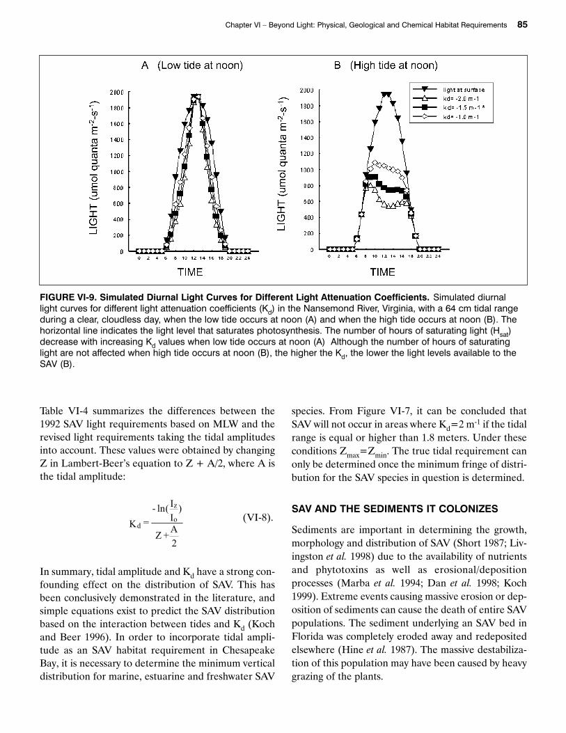
Tidal amplitudes in Chesapeake Bay (MHHW-MLLW) range from nontidal in some dammed tribu-taries to 50 cm in the upper Potomac River,Washington, DC, 60 cm in the Patuxent River, Mary-land and 64 cm in the Nansemond River, Virginia.SAV light requirements of Kd 1.5 and 2 m-1 were estab-lished in 1992 for Chesapeake Bay, based on a 1-meterrestoration depth (Batiuk et al. 1992). With this rela-tively high light attenuation, SAV would probably notexist if tidal ranges were higher than 1 meter (thisallows SAV to colonize a fringe between 75 and 40 cmin depth, respectively). From Figure VI-9a, it can beseen that, when the low tide at the Nansemond Riveroccurs at noon, the maximum light intensity resemblesthat of full sunlight but, the hours of saturating light(Hsat) decrease with increasing Kd. Figure VI-9b showsthe dramatic effect that a high tide at noon has on thelight availability to SAV in the Nansemond River. Thehigher the Kd, the less light is available to the SAVwhen the high tide is at noon. Figures VI-9a and VI-9bare based on a clear sunny day. If the day is cloudy, theeffect of a high tide at noon could lead the SAV to beexposed to light levels below saturation while a lowtide at noon could reduce the number of hours of sat-urating light that the plants receives even on a sunnyday by reducing the light available to the plants in theearly morning and late afternoon (high tides).

Tides have a significant effect on the light available toSAV in Chesapeake Bay, where tidal amplitudes arerelatively small but Kd values are relatively high. Inareas with lower Kd values in the past, an increase inKd, combined with high tidal amplitudes, can jointlycontribute to the decline of SAV distribution (Kochand Beer 1996).

The SAV light requirements presented in the first SAVtechnical synthesis (Batiuk et al. 1992) were estab-lished based on a restoration depth of 1 meter MLW(mean low water) without considering tidal range lev-els. This overestimated Zmax and underestimated thewater quality necessary to allow SAV to recolonizeareas down to a depth of 1 meter (Zmax = 1 meter).


FIGURE VI-7. Area-Specific Prediction of Vertical SAV Depth Distribution. An example of how this typeof graph can be used to predict the vertical distributionof SAV in a certain area. A tidal range of 0.8 m (see x-axis), a minimum light requirement of 13 percent(part of the equation to determine Zmax) and a Kd = 1.5 m-1 (see horizontal dashed lines) are assumed. A line is drawn vertically from the 0.8 m tidal range.The depth at which it intersects the diagonal linedetermines Zmin while the depth at which it intersectsthe horizontal dashed line for the selected Kd valuedetermines Zmax. In this case, SAV has the potential to grow in a fringe between 0.4 and 1.3 m deep. MTL is the mean tide level.

FIGURE VI-8. Illustration of Tidal Range Influenceson Vertical SAV Depth Distribution. Illustration of theSAV vertical depth distribution fringe determined inFigure VI-7. The fringe will occur in a 0.9 m depthinterval (1.3-0.4 m) due to tidal limitations at the topand light limitations at the bottom.

Table VI-4 summarizes the differences between the1992 SAV light requirements based on MLW and therevised light requirements taking the tidal amplitudesinto account. These values were obtained by changingZ in Lambert-Beer’s equation to Z + A/2, where A isthe tidal amplitude:

(VI-8).

In summary, tidal amplitude and Kd have a strong con-founding effect on the distribution of SAV. This hasbeen conclusively demonstrated in the literature, andsimple equations exist to predict the SAV distributionbased on the interaction between tides and Kd (Kochand Beer 1996). In order to incorporate tidal ampli-tude as an SAV habitat requirement in ChesapeakeBay, it is necessary to determine the minimum verticaldistribution for marine, estuarine and freshwater SAV

species. From Figure VI-7, it can be concluded thatSAV will not occur in areas where Kd=2 m-1 if the tidalrange is equal or higher than 1.8 meters. Under theseconditions Zmax=Zmin. The true tidal requirement canonly be determined once the minimum fringe of distri-bution for the SAV species in question is determined.

SAV AND THE SEDIMENTS IT COLONIZES

Sediments are important in determining the growth,morphology and distribution of SAV (Short 1987; Liv-ingston et al. 1998) due to the availability of nutrientsand phytotoxins as well as erosional/depositionprocesses (Marba et al. 1994; Dan et al. 1998; Koch1999). Extreme events causing massive erosion or dep-osition of sediments can cause the death of entire SAVpopulations. The sediment underlying an SAV bed inFlorida was completely eroded away and redepositedelsewhere (Hine et al. 1987). The massive destabiliza-tion of this population may have been caused by heavygrazing of the plants.

2A+Z

)II(ln-

=K o

z

d


FIGURE VI-9. Simulated Diurnal Light Curves for Different Light Attenuation Coefficients. Simulated diurnal light curves for different light attenuation coefficients (Kd) in the Nansemond River, Virginia, with a 64 cm tidal rangeduring a clear, cloudless day, when the low tide occurs at noon (A) and when the high tide occurs at noon (B). Thehorizontal line indicates the light level that saturates photosynthesis. The number of hours of saturating light (Hsat)decrease with increasing Kd values when low tide occurs at noon (A) Although the number of hours of saturatinglight are not affected when high tide occurs at noon (B), the higher the Kd, the lower the light levels available to theSAV (B).

On the other extreme, high sedimentation rates canalso be responsible for the decline of SAV populations.Moderate depositional rates can stimulate the growthof Thalassia testudinum (Gallegos et al. 1993) andCymodocea nodosa (Marba and Duarte 1994), buthigh depositional rates can lead to the disappearanceof these plants.

Seedlings are more susceptible to high burial ratesthan established SAV beds (Marba and Duarte 1994).Therefore, the season of depositional events is impor-tant in determining the chances of survival of SAVbeds. The deposition of more than 10 cm of sedimenton top of V. americana tubers reduced their chances ofbecoming mature plants and establishing a meadow(Rybicki and Carter 1986). Such high depositionalrates can occur during severe storms. In contrast, Z.marina seeds need to be buried at least 0.5 cm, where

conditions are anoxic, to promote germination (Mooreet al. 1993).

During less extreme conditions, SAV can modify thecharacteristics of the sediment it colonizes by reducingcurrent velocity and attenuating waves within its beds(see the review by Fonseca, 1996). This leads to thedeposition of small inorganic and light organic parti-cles (Kenworthy et al. 1982). The suitability of fine sed-iments and sediments with high organic content forSAV growth are addressed below.

Grain Size Distribution

Sediments within SAV beds are finer than those inadjacent unvegetated areas (Scoffin 1970; Wanless1981; Almasi et al. 1987). As SAV density increases,the ability to accumulate fine particles is alsoenhanced (due to the reduction in current velocity andwave energy). As grain size distribution becomesskewed toward silt and clay, the porewater exchangewith the overlying water column decreases. This mayresult in increased nutrient concentrations (Ken-worthy et al. 1982) and phytotoxins such as sulfide inmarine sediments (Holmer and Nielsen 1997). At theother extreme, if SAV colonizes coarse sand, theexchange of porewater with the overlying water col-umn will be enhanced and nutrient availability in thesediment may be lower than that of finer sediments.

In an experiment using different grain sizes of groundglass (to avoid adsorbed nutrients), Ruppia maritimawas found capable of colonizing sediments from asilt/clay mixture to coarse sand. Maximum growth wasobserved in fine and medium sand particles (Seeligerand Koch, unpublished data).

Table VI-5 lists quantitative and qualitative data onthe silt and clay amount found in healthy SAV beds.The values range from 0.4 to 90.1 percent. The highestvalues seem to be associated with beds in lower salin-ity environments with the exception of a Zostera muel-leri bed. Perhaps, in such environments, the plants areable to colonize sediment with reduced porewaterexchange with the water column because sulfide doesnot occur at the same levels as in marine/higher salin-ity estuarine systems. In higher salinity environments,it appears that plants need sediments that are moreoxygenated and in which sulfide levels can be reducedvia higher porewater advection rates. Therefore, SAV growth may be limited by the physical and


TABLE VI-4. Light attenuation requirements neces-sary for the recovery of SAV down to the 1 meterdepth contour, taking tides into account. Iz/Io (PLW)is assumed to be 13 percent for tidal fresh andoligohaline plants and 22 percent for mesohalineand polyhaline plants.


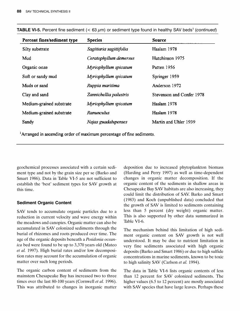
TABLE VI-5. Percent fine sediment (< 63 µm) or sediment type found in healthy SAV beds1

continued

geochemical processes associated with a certain sedi-ment type and not by the grain size per se (Barko andSmart 1986). Data in Table VI-5 are not sufficient toestablish the ‘best’ sediment types for SAV growth atthis time.

Sediment Organic Content

SAV tends to accumulate organic particles due to areduction in current velocity and wave energy withinthe meadows and canopies. Organic matter can also beaccumulated in SAV colonized sediments through theburial of rhizomes and roots produced over time. Theage of the organic deposits beneath a Posidonia ocean-ica bed were found to be up to 3,370 years old (Mateoet al. 1997). High burial rates and/or low decomposi-tion rates may account for the accumulation of organicmatter over such long periods.

The organic carbon content of sediments from themainstem Chesapeake Bay has increased two to threetimes over the last 80-100 years (Cornwell et al. 1996).This was attributed to changes in inorganic matter

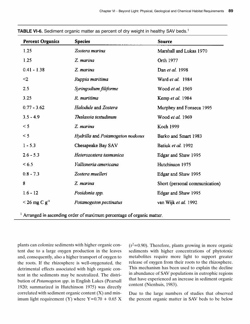
deposition due to increased phytoplankton biomass(Harding and Perry 1997) as well as time-dependentchanges in organic matter decomposition. If theorganic content of the sediments in shallow areas inChesapeake Bay SAV habitats are also increasing, theycould limit the distribution of SAV. Barko and Smart(1983) and Koch (unpublished data) concluded thatthe growth of SAV is limited to sediments containingless than 5 percent (dry weight) organic matter. This is also supported by other data summarized inTable VI-6.

The mechanism behind this limitation of high sedi-ment organic content on SAV growth is not wellunderstood. It may be due to nutrient limitation invery fine sediments associated with high organicdeposits (Barko and Smart 1986) or due to high sulfideconcentrations in marine sediments, known to be toxicto high salinity SAV (Carlson et al. 1994).

The data in Table VI-6 lists organic contents of lessthan 12 percent for SAV colonized sediments. Thehigher values (6.5 to 12 percent) are mostly associatedwith SAV species that have large leaves. Perhaps these


TABLE VI-5. Percent fine sediment (< 63 µm) or sediment type found in healthy SAV beds1 (continued)

plants can colonize sediments with higher organic con-tent due to a large oxygen production in the leavesand, consequently, also a higher transport of oxygen tothe roots. If the rhizosphere is well-oxygenated, thedetrimental effects associated with high organic con-tent in the sediments may be neutralized. The distri-bution of Potamogeton spp. in English Lakes (Pearsall1920; summarized in Hutchinson 1975) was directlycorrelated with sediment organic content (X) and min-imum light requirement (Y) where Y=0.70 + 0.65 X

(r2=0.90). Therefore, plants growing in more organicsediments with higher concentrations of phytotoxicmetabolites require more light to support greaterrelease of oxygen from their roots to the rhizosphere.This mechanism has been used to explain the declinein abundance of SAV populations in eutrophic regionsthat have experienced an increase in sediment organiccontent (Nienhuis, 1983).

Due to the large numbers of studies that observed the percent organic matter in SAV beds to be below


TABLE VI-6. Sediment organic matter as percent of dry weight in healthy SAV beds.1

5 percent, it is recommended that caution should betaken when transplanting SAV into areas where thesediment organic content is higher than that value.Additional studies are needed to define the SAV habi-tat requirement for organic matter for different SAVspecies in Chesapeake Bay.

SAV AND SEDIMENT GEOCHEMISTRY

Nutrients in Sediments

Nutrients in the sediment can be limiting to thegrowth of SAV (Short 1987; Agawin et al. 1996) but donot seem to eliminate it from colonizing certain areas.In marine siliceous sediments, nitrogen may limit SAVgrowth (Short 1987; Alcoverro et al. 1997) while inmarine carbonate sediments, phosphorus may be lim-iting to SAV growth (Wigand and Stevenson 1994).Potassium has been suggested to be limiting to thegrowth of freshwater SAV (Anderson and Kalf 1988).Mycorrhizae have been found to facilitate the phos-phorus assimilation in V. americana (Wigand andStevenson 1997), but little or no information is avail-able on mycorrhizae in the rhizosphere of marine SAV(Wigand and Stevenson 1994).

Although light seems to be more limiting to SAVgrowth than sediment nutrient concentrations, excep-tions can be found. In tropical SAV beds, light andtemperature are limiting in the winter while nutrientsare limiting in the summer (Alcoverro et al. 1997b).Additionally, ammonium concentrations as low as 25 µm (in the seawater) can be toxic to Z. marinaand ultimately lead to its decimation (van Katwijk et al. 1997).

Microbial-Based Phytotoxins

A wide variety of potentially phytotoxic substances isproduced by bacterial metabolism in anaerobic sedi-ments, including phenols and organic acids, reducediron and manganese and hydrogen sulfide (Yoshida1975; Gambrell and Patrick 1978). In many aquaticenvironments, sulfide probably constitutes the mostimportant of these toxic bacterial metabolites and hasbeen shown to be toxic to estuarine and marine SAVspecies (van Wijck et al. 1992; Carlson et al. 1994).

Sulfide is generated by sulfate reducing bacteria dur-ing organic carbon oxidation and nutrient remineral-ization in anoxic sediments (Howarth 1984; Pollardand Moriarty 1991). A high remineralization rate leadsto high nutrient availability and favors plant growthbut can also lead to the accumulation of sulfide, whichis detrimental to plant growth. Sulfate remineraliza-tion depends on the temperature and amount oforganic matter in the sediment. In freshwater sedi-ments, sulfate reduction is less important thanmethanogenesis due to the lower sulfate availability.As SAV tends to accumulate more organic and inor-ganic particles than unvegetated areas, sulfate reduc-tion rates can be expected to be higher within thevegetation than outside it (Isaksen and Finster 1996;Holmer and Nielsen 1997). This difference could alsobe due to the excretion of organic compounds throughthe roots (Blackburn et al. 1994).

Table VI-7 summarizes sulfide levels observed inhealthy as well as deteriorating SAV beds, and TableVI-8 lists sulfate reduction rates in healthy SAV beds.While eutrophication can fuel sulfide production viaincreased organic matter in the sediments, sulfide pro-duction can also fuel eutrophication. The sulfide pro-duced inhibits nitrification (NH4

+ → NO3–) and,

consequently, increases ammonium fluxes to the watercolumn, which could act as a positive feedback toeutrophication (Joye and Hollibaugh 1995).

A parallel mechanism also applies to the release ofphosphorus from the sediments. When sulfides reactwith iron in the sediment, iron sulfide is formed andphosphorus is released (Lamers et al. 1998). If thephosphorus is not taken up by the plants, it may bereleased back into the water column and, as statedabove for nitrogen, may be a positive feedback toeutrophication.

The toxicity of sulfide to plants can also be enhancedby eutrophication. Oxygen released from SAV roots isneeded to oxidize the sulfide and reduce its toxiceffects (Armstrong 1978). The release of oxygen by theroots depends on the photosynthetic rates of the plant.Therefore, if eutrophication leads to a reduction inlight availability, photosynthetic rates will be lower,the amount of oxygen released from the roots will alsobe reduced and sulfide toxicity may be enhanced(Goodman et al. 1995).



TABLE VI-7. Sulfide levels in the sediments of healthy and dying SAV beds.

TABLE VI-8. Sulfate reduction in healthy SAV beds.

Sulfide concentration in the sediment is an importantSAV habitat requirement. Correlations between pore-water sulfide concentrations and the growth of severalSAV species have indicated that concentrations above1 mM may be toxic (Pulich 1989; Carlson et al. 1994).Direct manipulations of sulfide concentrationsrevealed a negative effect on photosynthesis (Good-man et al. 1995) and growth (Kuhn 1992) when levelswere higher than 1 to 2 mM. Sulfide thresholds for dif-ferent SAV species (in combination with different lightlevels) still need to be determined. Until such data areavailable, critical sulfide concentrations cannot bespecified as an SAV habitat requirement.

CHEMICAL CONTAMINANTS

This review is intentionally confined to the broadissues of the potential roles contaminants may have inlimiting the size, density and distribution of SAV pop-ulations. Literature values pertaining to the relation-ships between SAV and chemical contaminants arederived from three diverse lines of inquiry: contami-nant studies, phytoremediation efforts (Garg et al.1997; Peterson et al. 1996; Ramanathan and Burks

1996; Salt et al. 1995), and recommendations foraquatic weed control (Anderson and Dechoretz 1982;Anderson 1989; Nilson and Klaassen 1988). AppendixB summarizes some of the more recent work devotedto contaminant issues.

Most of the chemical contaminant studies have evalu-ated the effects of herbicides on SAV growth (Fleminget al. 1993). A few have examined other pesticides orheavy metals (Garg et al. 1997; Gupta and Chandra1994; Gupta et al. 1995). Thus, the vast majority of com-pounds known to have toxic effects on biological sys-tems remain untested (Van Wijngaarden et al. 1996)and only a few efforts have been made to systematicallyevaluate additive, cumulative and synergistic effects ofmultiple contaminants (Fairchild et al. 1994; Huebertand Shay 1992; Sprenger and McIntosh 1989).

Nonetheless, the following conclusions can be drawnfrom these accumulated data.

• Herbicides have been shown to be phytotoxic toSAV. Toxicity is somewhat species-dependent andchemical-specific. Table VI-9 depicts the toxicityrange of the most widely used herbicides in the


TABLE VI-9. Relative effects of herbicides on net photosynthesis in Potamogeton pectinatus. The IC50 isthe predicted concentration that inhibits photosynthesis by 50%. Photosynthesis was determined bymeasuring O2 production by plants over 3 hours at 20-22°C and about 58% µmol/m2/sec of photosyntheti-cally active radiation from full spectrum fluorescent lighting. Plants were exposed to herbicides added tothe water column. Reprinted with permission: W. James Fleming 1993.

United States on Potamogeton pectinatus. Inhibit-ing concentrations range from 8 ppb to 10,000ppb. These concentrations are consistent withthose observed when aquatic weed control is themanagement objective, as well as in environ-ments where the protection of aquatic plants isthe management objective.

• Pesticides other than herbicides have been shownto have a phytotoxic effect on SAV, although onlya few have been evaluated.

• Heavy metals at levels corresponding to someambient conditions have inhibiting effects onSAV in test systems where the variety of essentialplant nutrients has been experimentally factored.

• The environments holding the greatest potentialfor pesticide suppression of SAV populations areheadwaters and shallow waters immediately adja-cent to the urban, forest and agricultural areaswhere pesticides are most widely used and acuteconcentration level exposures are most likely to occur.

• The environments holding the greatest potentialfor adverse effects of heavy metals are those

where clay and organic sediments chemicallyconcentrate both metals and plant nutrients forextended periods.

• The utility of ambient testing of contaminantconcentrations is highly controversial. For pesti-cides, the constraint of monitoring frequency andlocation are limiting factors for accurate ambientassessment of contaminant presence. Assessmentof heavy metals and other contaminants is con-founded by the difficulty of distinguishingbetween the concentration of biologically activeforms and total concentration (Liang and Schoe-nau 1996).

PHYSICAL AND GEOLOGICAL SAV HABITATREQUIREMENTS

In order to fully define the SAV habitat requirementsin Chesapeake Bay, parameters other than light and itsmodifiers need to be taken into consideration. Somephysical, geological and geochemical parameters havethe potential to override established SAV lightrequirements. Where field and laboratory experimen-tal data were sufficient, physical and geological SAVhabitat requirements were identified (Table VI-10).



TABLE VI-10. Summary of physical and geological SAV habitat requirements for Chesapeake Bay.

Date post:	18-Dec-2021
Category:	Documents
Upload:	others
View:	1 times
Download:	0 times

CHAPTER VI Beyond Light: Physical, Geological and Chemical ...

Documents